Fractals/Computer graphic techniques/2D/exp

Disambiguation

Exponential mapping of the plane is:

• is exponential transformation of the plane

Exponential mapping of the plane is not

• the Julia set or Mandelbrot set of the exponential function ( exponentia map), like Exponential Mandelbrot z := exp(z) + c
• Logarithmic scale on one axis
• Logarithmic scale on both axes: Log-log scale plot
• polar azimuthal equidistant projection ( Exponential map in Riemannian geometry)
• The exponential operator, anamorphosis operator which can be applied to grayscale images.

Compare exponential function by different input

• single number ( 0D space) gives natural exponent of the number
• number line ( 1D space). Exponential scale is not used. Logarithmic scale is used for exponential data. It gives a linear function.
• plane ( 2D space) gives exponential mapping

number

In mathematics, the logarithm is the inverse function to exponentiation. That means the logarithm of a number x to the base b is the exponent to which b must be raised, to produce x

$y=\log _{b}x$

is equivalent to

$x=b^{y}$

if b is a positive real number. (If b is not a positive real number, both exponentiation and logarithm can be defined but may take several values, which makes definitions much more complicated.)

• 
  a logarithm function and an exponential function
• 
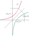
  Plots of logarithm functions, with three commonly used bases. The special points log_b b = 1 are indicated by dotted lines, and all curves intersect in log_b 1 = 0
• 
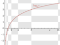  The graph of the logarithm base 2 crosses the x-axis at x = 1 and passes through the points (2, 1), (4, 2), and (8, 3), depicting, e.g., log₂(8) = 3 and 2³ = 8. The graph gets arbitrarily close to the y-axis, but does not meet it

The real exponential function is a bijection from $\mathbb {R}$ to $(0;\infty )$. Its inverse function is the natural logarithm, denoted $\ln ,\log ,\log _{e};$ because of this, some old texts refer to the exponential function as the antilogarithm.

scale

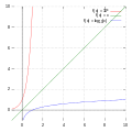
A logarithmic scale (or log scale) is a way of displaying numerical data over a very wide range of values in a compact way—typically the largest numbers in the data are hundreds or even thousands of times larger than the smallest numbers. Such a scale is nonlinear: the numbers 10 and 20, and 60 and 70, are not the same distance apart on a log scale. Rather, the numbers 10 and 100, and 60 and 600 are equally spaced. Thus moving a unit of distance along the scale means the number has been multiplied by 10 (or some other fixed factor). Often exponential growth curves are displayed on a log scale, otherwise they would increase too quickly to fit within a small graph. Another way to think about it is that the number of digits of the data grows at a constant rate. For example, the numbers 10, 100, 1000, and 10000 are equally spaced on a log scale, because their numbers of digits is going up by 1 each time: 2, 3, 4, and 5 digits. In this way, adding two digits multiplies the quantity measured on the log scale by a factor of 100.

Logarithmic scale

• on 1 axis = semi-log plot
  • linear-log plot
  • log-linear plot
• on both axes = log-log plot

• 
  Lin-Lin scale
• 
  Log-Lin scale
• 
  Lin-Log scale
• 
  Log-Log scale

Logarithmic scale is used for exponential data. It gives a linear function.

The function of f(x) = 2^x plotted on the logarithmic scale looks like linear function

mapping

• GRAPHICS FOR COMPLEX ANALYSIS by Douglas N. Arnold:
  • "the complex exponential maps the infinite open strip bounded by the horizontal lines through +/- pi i one-to-one onto the plane minus the negative real axis.
  • The lines of constant real part are mapped to circles, and lines of constant imaginary part to rays from the origin.
  • In the animation we view a rectangle in the strip rather than the entire strip, so the region covered is an annulus minus the negative real axis.
  • The inner boundary of the annulus is so close to the origin as to be barely visible.
  • We also make the strip a bit thinner than 2 pi, so that the annulus does not quite close up."
  • the complex exponential map takes the rectangle |Re(z)| ≤ a, |Im(z)| ≤ π onto the annulus $e^{-a}\leq |w|\leq e^{a}$
• Composition of complex Mappings Viewer by Paul Falstad - the composition of selected mapping functions: g(f(z)). One have to increase grid size to have tha same effect ( rectangle to annulus mapping)
• The Complex Exponential Function Author:Susan Addington
• Complex mappings Author:Juan Carlos Ponce Campuzano
• Complex exponential function Author:Tatsuyoshi Hamada : Complex exponential function maps rectangular domain to fan shaped image ( part or full sector of punctured circle )
• Complex exponential map by Siamak on geogebra:
  • vertical axis is transformed to the circle on the w-plane
  • horizontal axis is is transformed to the radii on the w-plane
• Images of a square grid of size [-3,3]x[-3,3] under the (conformal) exponential map givers almost full annulus
• The complex exponential function mapping biholomorphically a rectangle [-1,1]x[0 ,pi/2] to a quarter-annulus $[e^{-1},e]x[e^{-1},e]$
• 24 Views of the Complex Exponential Function by Pacific Tech
• mathematica question: how-do-i-visualize-expz-as-a-complex-mapping

• virtual math museum: ConformalMaps, complex exponential function:"a Cartesian Grid is mapped “conformally” (i.e., preserving angles) to a Polar Grid: the parallels to the real axis are mapped to radial lines, and segments of length 2π that are parallel to the imaginary axis are mapped to circles around 0."

exp(x + i · y) = exp(x) · exp(i · y) = exp(x) · cos(y) + i · exp(x) · sin(y)

• Surfaces representing the complex exponential
• 
  real part
• 
  imaginary part
• 
  modulus = cabs
• 
  main argument = carg

• Density curve representing of the complex exponential
• 
  real part
• 
  imaginary part

• exponential mapping
• 
  The Log-Polar Mapping. Point (x,y) is mapped to $(\rho ,\theta )$ where $\rho =\log {\sqrt {x^{2}+y^{2}}}$ and $\theta =\arctan({\frac {y}{x}})$. In general circles around orogin and radii are mapped to horizontal and vertical lines.
• 
• 
  mercator projection vs rotation
• 
  the exponential mapping from the tangent space to the sphere

3D	2D	description
$f(z)=\exp(z)$	$f(z)=\exp(z)$
$f(z)=\log(z)$	$f(z)=\log(z)$

period

The exponential function is periodic:

exp(z + 2 π * i) = exp(z). 

The periodicity is also clear from the formula:

exp(x + i * y) = exp(x) * (cos(y) + i * sin(y)) .

The graph of the exponential function is a two-dimensional surface ( x,y) that curves through four dimensions ( x,y,v,w).

• 
  v+iw = exp(x+iy) for values of x from -1.5 to 1.5 and values of y from -2π to 2π, so that shows two complete rotations of the spiral.

Name

• exponential mapping
• the exponential map
• Mercator ( it is not good name because here is only mapping from flat complex plane ( 2D Cartesian plane) to exponential plane. Here there is no mapping from sphere to flat complex plane ( Cartesian plane) )
  • Mercator map
  • Mercator projection
• polar projection
• log-polar mapping ( Log-polar coordinates )
• logarithmic
  • logarithmic projection around a point c0: z-> (log(|z-c0|)
• log(z)-Mandelbrot-Zooms = side scrolling ( side scrolling fractal zoom )

General names:

• graphical projection
• geometric transformation

Description

Math notation $map:\mathbb {C} \to \mathbb {C}$ $c_{e}\leftarrow e^{c}+c_{0}$

// c with complex type complex double map(complex double c) { return c_e = cexp(c) + c0; }

// c without complex type cx_e = exp(creal(c)) * cos(cimag(c)) + realpart(c0); // real part of c_e cy_e = exp(creal(c)) * sin(cimag(c)) + imagpart(c0); // imag part of c_e

Features

Maps

• Rectangle of Cartesian plane to quadratic sectors of polar coordinate,
• x is mapped to radius, and y to angle ( radians)

• horizontal
  • maps $c_{0}$ to infinity ( limit of the sequence = MF = the Myrberg-Feigenbaum point = the Feigenbaum Point)
  • maps important components related with above sequence to the same size
• vertical
  • vertical coordinate are periodic of period $2\pi$, because they use trigonometric functions

Examples:

• sequence of root points for periods $p=1*2^{n}$ ( period doubling cascade) and the limit point of the sequence is the Myrberg-Feigenbaum point $\mathbf {MF} _{1/2}=c_{0}=-1.401155...$
• sequence of root points for periods $p=1*3^{n}$ and the limit point of the sequence is the Myrberg-Feigenbaum point $\mathbf {MF} =c_{0}=-1.7864402555636388747...$

• 
• 

Informal description

• The exponential mapping transforms the entire complex plane into a strip that has unlimited length along the real axis, and a width of 2π along the imaginary axis. Exponential Map from the Mandelbrot Set Glossary and Encyclopedia, by Robert Munafo, (c) 1987-2022
• " The idea is to focus on a point in or near the Mandelbrot set, and create an image where one direction is the logarithm of the distance and the other one the angle. The result is very much like the astro-ph/031571 map and theXKCD cartoon versions. This map projection is conformal, so it does not distort local angles, and objects are usually recognizable on all scales." Anders Sandberg
• Images of the Mandelbrot set with a logarithmic projection around a point c0: z-> (log(|z-c0|), arg(z-c0)). Anders Sandberg
• "it is a log map toward the target point (or, as some might say, a Mercator projection with the target point as South pole and complex ∞ as North pole); horizontally it is periodic and I have placed two periods side to side, whereas vertically it extends to infinity at the top and at the bottom, which corresponds to zooming infinitely far out or in, at a factor of exp(2π)≈535.5 for every size of a horizontal period. Horizontal lines (“parallels”) on the log map correspond to concentric circles around the target point, and vertical lines to radii emanating from it; and the anamorphosis preserves angles." David Madore
• "The coordinate system is such that the angular component goes to the y-axis, and the radius goes to the x-axis of the resulting image. In addition, the x-axis (radius) is normalized with exp-function so that angles are preserved in this mapping. " Mika Seppä
• log : "To illustrate the complexity of the boundary of the Mandelbrot set, Figure 8 renders the image of dM under the transformation log(z - c) for a certain c in the boudary of Mandelbrot set. Note the cusp on the main cardioid in the upper right; looking to the left in the figure corresponds to zooming in towards the point c. (Namely, c = -0.39054087... - 0.58678790i... the point on the boundary of the main cardioid corresponding to the golden mean Siegel disk.). Note the cusp on the main cardioid in the upper right; looking to the left in the figure corresponds to zooming in towards the point c. "
• "Legendary side scrolling fractal zoom. 1 Month + (Interpolator+Video Editor) = Log(z). This means logarithmic projection for this location, that gives this interesting side-scrolling plane ^^)"
• " There are no program that can render this fractal on log(Z) plane. But you can make it in Ultra Fractal or in similar software with programmable distributive. Formula is:C = exp(D), for D - is your zoomable coordinates" SeryZone X
• just c = c0 + cexp(x + i y) and x + i y = clog(c - c0), with scaling by 2pi/width (Claude)
• idea
  • A Map of the Universe by J. Richard Gott III, Mario Jurić, David Schlegel, Fiona Hoyle, Michael Vogeley, Max Tegmark, Neta Bahcall, Jon Brinkmann
  • XKCD cartoon versions

Formal mathematical description

Complex log and exp mapping

Forward transformation

Here transformation is a composition of 2 transformations:

• complex exponential function: $f(c)=e^{c}$
• geometric or complex translation $t(x)=x+c_{0}$

 $c_{e}=t(f(c))$

$c_{e}\leftarrow e^{c}+c_{0}$

where:

• c is a parameter point from c plane ( flat image in Cartesian coordinate = linear scale on both axes). It is a a parameter of quadratic map $z^{2}+c$
• $c_{e}$ is a parameter in a new transformed plane ( log-polar image )
• $c_{0}$ is a constant parameter (for translation). It is sometimes called center, but better name seems to be: target or limit point
• e is Euler's number, is a mathematical constant approximately equal to 2.71828,

Inverse transformation:

$c=ln(c_{e}-c_{0})$

where:

• $ln$ is natural logarithm

exp

Complex exponential map

The complex exponential function is periodic with period 2πi and $\exp(z+2\pi ik)=\exp z$ holds for all $z\in \mathbb {C} ,k\in \mathbb {Z}$.

The exponential function maps any line in the complex plane to a logarithmic spiral in the complex plane with the center at the origin. Two special cases exist:

• when the original line is parallel to the real axis, the resulting spiral never closes in on itself;
• when the original line is parallel to the imaginary axis, the resulting spiral is a circle of some radius.

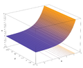
Considering the complex exponential function as a function involving four real variables:

$$v+iw=\exp(x+iy)$$

the graph of the exponential function is a two-dimensional surface curving through four dimensions.

Starting with a color-coded portion of the $xy$ domain, the following are depictions of the graph as variously projected into two or three dimensions.

• Graphs of the complex exponential function
• 
  Checker board key:
  $x>0:\;{\text{green}}$
  $x<0:\;{\text{red}}$
  $y>0:\;{\text{yellow}}$
  $y<0:\;{\text{blue}}$
• 
  Projection onto the range complex plane (V/W). Compare to the next, perspective picture.
• 
  Projection into the $x$, $v$, and $w$ dimensions, producing a flared horn or funnel shape (envisioned as 2-D perspective image).
• 
  Projection into the $y$, $v$, and $w$ dimensions, producing a spiral shape. ($y$ range extended to $\pm 2\pi$, again as 2-D perspective image)

The second image shows how the domain complex plane is mapped into the range complex plane:

• zero is mapped to 1
• the real $x$ axis is mapped to the positive real $v$ axis
• the imaginary $y$ axis is wrapped around the unit circle at a constant angular rate
• values with negative real parts are mapped inside the unit circle
• values with positive real parts are mapped outside of the unit circle
• values with a constant real part are mapped to circles centered at zero
• values with a constant imaginary part are mapped to rays extending from zero

The third and fourth images show how the graph in the second image extends into one of the other two dimensions not shown in the second image.

The third image shows the graph extended along the real $x$ axis. It shows the graph is a surface of revolution about the $x$ axis of the graph of the real exponential function, producing a horn or funnel shape.

The fourth image shows the graph extended along the imaginary $y$ axis. It shows that the graph's surface for positive and negative $y$ values doesn't really meet along the negative real $v$ axis, but instead forms a spiral surface about the $y$ axis. Because its $y$ values have been extended to ±2π, this image also better depicts the 2π periodicity in the imaginary $y$ value.

Log

Complex logarithm as a conformal map

Since a branch of $\log z$ is holomorphic, and since its derivative $\log z$ is never 0, it defines a conformal map.

For example, the principal branch $w=\operatorname {Log} z$, viewed as a mapping from $\mathbb {C} -\mathbb {R} _{\leq 0}$ to the horizontal strip defined by $\left|\operatorname {Im} z\right|<\pi$, has the following properties, which are direct consequences of the formula in terms of polar form:

• Circles in the z-plane centered at 0 are mapped to vertical segments in the w-plane connecting $a-\pi i$ to $a+\pi i$, where $a$ is the real log of the radius of the circle.
• Rays emanating from 0 in the z-plane are mapped to horizontal lines in the w-plane.

Each circle and ray in the z-plane as above meet at a right angle. Their images under Log are a vertical segment and a horizontal line (respectively) in the w-plane, and these too meet at a right angle. This is an illustration of the conformal property of Log.

Complex log mapping maps radii to horizontal lines and circles to vertical lines

description for programmers

// https://code.mathr.co.uk/mandelbrot-graphics/blob/HEAD:/c/lib/m_d_transform.c
static void m_d_transform_exponential_forward(void *userdata, double _Complex *c, double _Complex *dc) {
  m_d_transform_exponential_t *t = userdata;
  double _Complex c0 = *c;
  double _Complex dc0 = *dc;
  *c = cexp(c0) + t->center;
  *dc = dc0 * cexp(c0);
}


static void m_d_transform_exponential_reverse(void *userdata, double _Complex *c, double _Complex *dc) {
  m_d_transform_exponential_t *t = userdata;
  double _Complex c0 = *c;
  double _Complex dc0 = *dc;
  *c = clog(c0 - t->center);
  *dc = dc0 / (c0 - t->center);
}

Filter Mercator from MathMap

filter mercator (image in)
   in(xy*xy:[cos(pi/2/Y*y),1])
end

Maxima CAS src code:

(%i1) kill(all);
(%i2) display2d:false;
(%i3) ratprint : false; /* remove "rat :replaced " */
(%i4) c:cx +cy*%i$
(%i5) c0:c0x+c0y*%i$
(%i6) realpart(c0 + exp(c));
(%o6) %e^cx*cos(cy)+c0x
(%i7) imagpart(c0 + exp(c));
(%o7) %e^cx*sin(cy)+c0y
(%i8) cabs(c0 + exp(c));
(%o8) sqrt((%e^cx*sin(cy)+c0y)^2+(%e^cx*cos(cy)+c0x)^2)
(%i9) carg(c0 + exp(c));
(%o9) atan2(%e^cx*sin(cy)+c0y,%e^cx*cos(cy)+c0x)

Notes

• the mapping is periodic because there are trigonometric functions inside

(%i1) kill(all);
(%i2) display2d:false;
(%i3) ratprint : false; /* remove "rat :replaced " */
(%i4) ce:ceex+cey*%i;
(%i5) c0:c0x+c0y*%i;
(%i6) realpart(log(ce - c0));
(%o6) log((cey-c0y)^2+(ceex-c0x)^2)/2
(%i7) imagpart(log(ce - c0));
(%o7) atan2(cey-c0y,ceex-c0x)

// https://www.foerstemann.name/dokuwiki/doku.php?id=log_z_-mandelbrot-zooms
// log(z)-Mandelbrot-Zooms by 
<languageVersion: 1.0;> 
kernel zoomer
< namespace : "Zoomer"; vendor : "private"; version : 2; description : "zoomer 2"; >
{
  const float PI = 3.14159265;
  const float EU = 2.71828; 
  parameter float translate <       
      minValue:float(0);
      maxValue:float(400.0); 
      defaultValue:float(0.0); >;
  parameter float rotate <       
      minValue:float(0.0);
      maxValue:float(960.0); 
      defaultValue:float(0.0); >;
  input image4 iImage1;
  input image4 iImage2;
  input image4 iImage3;
  input image4 iImage4;
  output float4 outputColor;
  void evaluatePixel()
  {
      float2 position = outCoord() - float2(479.5,199.5);
      float2 tmp = outCoord();
      tmp.y = abs(log(sqrt(pow(position.x,2.0) + pow(position.y,2.0))/510.0))*30.474;
      tmp.x = mod((atan(position.x, position.y)/PI + 1.0)*480.0, 958.5) ;
      position = tmp + float2(rotate,translate);
      position.x = mod(position.x,958.5)+1.0;
      if ( position.y < 398.5) {outputColor = sampleLinear( iImage1, position );} 
      else if ( position.y < 797.0) {outputColor = sampleLinear( iImage2, position - float2( 0.0 , 398.0 ));} 
      else if ( position.y < 1199.5) {outputColor = sampleLinear( iImage3, position - float2( 0.0 , 796.0 ));}
      else {outputColor = sampleLinear( iImage4, position - float2( 0.0 , 1194.0 ) );}  
  }
}

center

$c_{0}$ is a constant parameter (for translation = offset).

It is sometimes called center, but better name seems to be:

• target
• limit point
• offset or translation

The target point ( center) is projected onto -∞+0i in the exponential-mapped view. It would be intinitely far to the left and it is not seen on the image.

zoom

• the leftmost column of the image has the minimal zoom ( the biggest plane radius )
• the rightmost column of the image has the maximal zoom ( the smallet plane radius )

exponential grid scan

Conventions:

• Robert Munafo generate the angle based on the horizontal pixel coordinate, and the radius from the vertical pixel coordinate ( image is in the vertical position , it is standing on the shorter dimension)
• the normal way is to have the angle come from the vertical pixel coordinate ( image is in the horizontal position , it is lying on the longer dimension)

The grid scan with exponential coordiante mapping is different then the standard scan for flat images.

for (int j = 0; j < h; ++j) { // vertical coordinate = number of the rows
    
     double e_angle = ((double) j) * px / r * 3.14159265359;  // Robert's way:  angle from 0 to 2π. 
   
   for (int i = 0; i < w; ++i) { // horizontal coordinate = number of the columns
    
       e_radius = ((double) i) * px / r * 3.14159265359;
       .....
    }

Description

• image_width is the maximal number of pixels = width of the image in pixels ( integer number)

Here:

• pixel coordinate j is going from 0 to image_height - 1
• so j/pixel_height goes from 0.0 to 1.0
• therfore angle goes from 0 to 2 pi

Claude's way is mathematically correct: the angle is usually thought of as going from -π to π, not from 0 to 2π. To fix this part, you can adjust your pixel coordinate right before computing an angle from it. Change this:

double e_angle = ((double) j) * px / r * 3.14159265359;

to this:

double e_angle = ((double) (j-h/2)) * px / r * 3.14159265359;

Notes

• e_radius is a linear function of i
• e_angle is a linear function of j

computing pixel coordinate

Here is example by by Robert Munafo

   /* Inputs are:
     ctr_r is the real coordinate of the center of the view we want to plot
     ctr_i is the imaginary coordinate of the center of the view
     
     real_width is the width of the image (in real coordinates). this should reflect the width when "zoomed in" all the way
     
     pixel_width is the number of pixels per row of the image we want to create
     pixel_height is the number of rows of pixels, or pixels per column
  
     This setup code computes:
     px_spacing is the width of the image (in real coordinate)
       divided by the number of pixels in a row
     halfwidth is half the width of the image (in real coordinate)
     halfheight is half the height of the image (in imaginary coordinate)
     min_r is the real coordinate of the left edge of the image
     max_i is the imaginary coordinate of the top of the image
  */
  void setup()
  {
    px_spacing = real_width / pixel_width;
    halfwidth = real_width / 2.0;    
    halfheight = halfwidth * pixel_height / pixel_width;
    min_r = ctr_r - halfwidth;
    max_i = ctr_i + halfheight;
  }
  

  /* Plot a single pixel, row i and column j. Use as many rows as you need
     for the image to show the whole Mandelbrot set. */
  void pixel_53(int i, int j, int itmax)
  {
    double cr, ci, offset_r, offset_i, angle, log_radius;
  
    /* compute angle and radius. Note that pixel_width is the number of
       pixels wide of the image, and j goes from 0 to pixel_width-1. This
       means that "j/pixel_width" goes from 0.0 to 1.0, and therefore
       angle goes from 0 to 2 pi. log_radius needs to be computed the
       same way in order for shapes to be preserved, which happens because
       the complex exponential function is a conformal map.
    Important: the row coordinate i can be as big as you want: add as many
       rows of pixels as are needed for the "log_radius" to get close to 1.
       This ensures that exp(log_radius) gets big enough to go beyond the
       area that has the Mandelbrot set in it. */
    angle =      (((double) j) / pixel_width) * 2.0 * 3.14159265359;
    log_radius = (((double) i) / pixel_width) * 2.0 * 3.14159265359;
  
    /* compute offsets = translation = add complex number offset */
    offset_r = cos(angle) * halfwidth * exp(log_radius);
    offset_i = sin(angle) * halfwidth * exp(log_radius);
  
    ci = ctr_i + offset_i;
    cr = ctr_r + offset_r;
    evaluate_and_plot(cr, ci, itmax, i, j);
  }

Compare with

• exponential strip by Claude Heiland-Allen: The rendering of the final video can be accelerated by computing exponentially spaced rings around the zoom center, before reprojecting to a sequence of flat images. In case of problems : https://mathr.co.uk/mandelbrot/exponential_strip.svg

aspect ratio

• For best (more conformal) results use a wide aspect ratio (9:1 works well, window size 1152x128 or 1536x170).

scale factor R

To minimize the total number of pixels that need calculating, which is proportional to

$K={\frac {R^{2}-1}{logR}}$

Define the efficiency of zoom by

${\frac {2}{K}}$

then:

• the traditional R=2 has an efficiency of only 46%,
• R=4/3 has 74%
• R=8/7 has 87% efficacy

where

• video image size is W×H

Videos

• Mercator - Scrolling Mandelbrot Fractal by Mathtown
• Mappings by the exponential function by William Nesse
• Mapping properties of the exponential function by MatheMagician
• The function f(z)=exp(z) by Michael Robinson
• Complex: visualizing exponential map and local inverse by James Cook
• Mandelbrot Mercator Testing by Fractal MathPro

Images

• Category:Mandelbrot sets - Mercator projection in commons

• 
  without transformation
• 
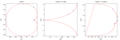
  real (= 1D) version
• 
  1D: 3 windows with non-linear, i.e. logarithmic x-axis scale:
• 
  complex (= 2D) version
• 
  normal projection
• 
  polar projection
• 
  M(3,1) Misiurewicz at 1E10 magnification (bottom) use the exponential map
• 
• 
  Mercator Effect in GIMP with MathMap

2 images with the same parmeter. In the upper image main antenna is on both sides, in the lower one in the center of the image

• Mercator
• 
  Map of the region close to the Myrberg-Feigenbaum point. The buds of the main Mandelbrot set converge geometrically towards this place (at a rate set by Feigenbaum's constant), producing the regularly spaced buds at the top and bottom. Since I did not have an exact coordinate for it, the map is centered a little bit away.
• 
  This image corresponds to a 10^30 zoom around a point (I just used 30 digits of precision, so there are artefacts at the left edge
• 
  This image corresponds to a 10^30 zoom around a point (I just used 30 digits of precision, so there are artefacts at the left edge).
• 
  10^60 zoom. The banded structure occurs because the zoom passes through the embedded Julia sets around smaller Mandelbrot sets; each new Mandelbrot zoomed past adds their own Julia set to the sequence. The center point is c=-1.256827152259138864846434197797294538253477389787308085590211144291 +0.37933802890364143684096784819544060002129071484943239316486643285025i
• 
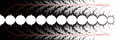
  Zooms of the Mandelbrot set around a point projected so that the distance to the point forms a logarithmic scale. Details on the left edge are ~10^15 times smaller than on the right edge. The rightmost black blob in the pictures is the main "continent" of the set. Satelite sets of different sizes can be seen linked by fractal chains of varying complexity. The colors are set using the distance estimator method.

How to read location from exponential image ?

• fractalforums.org : can-you-find-the-location-of-this-fractal ?
• "An inverse mapping (using the complex logarithm function) is used to compute the location (in the strip) of needed data for any given location in the normal orthogonal coordinate space." Robert Munafo

Tips:

• the image is not symmetric ( up and down) so imaginary part of c0 is not zero

Implementations

Fractal programs

• fraktaler-3
• UltraFractal
• Polar_Projection in fractalzoomer
• Fractalshades - python program by Geoffroy Billotey
• emndl: exponential strip visualisation of the Mandelbrot set, program by Claude Heiland-Allen
• pfract - console c program by Mika Seppä
• emndl: mathr's exponential strip mandelbrot set renderer: it is: c = c0 + cexp(x + i y) and x + i y = clog(c - c0), with scaling by 2pi/width
• Fractalshades doc : P01-feigenbaum expmap

Kalles Fractaler and zoomasm

• The rendering of the final video can be accelerated by computing exponentially spaced rings around the zoom center, before reprojecting to a sequence of flat images.
• kf-2.15 supports rendering EXR keyframes in exponential map form
• zoomasm can assemble above keyframes into a zoom video. zoomasm works from EXR, including raw iteration data, and colouring algorithms can be written in OpenGL shader source code fragments
• kf-extras by Claude Heiland-Allen - has the exponential map (aka log polar or mercator projection) convertor

OpenCV

• opencv 3.4 warpPolar() function
• logpolar transform using Camera by Aresh T. Saharkhiz
• stackoverflow question: reprojecting-polar-to-cartesian-grid
• descr
• stackoverflow question: how-to-tune-log-polar-mapping-in-opencv
• stackoverflow question : converting-an-image-from-cartesian-to-polar-limb-darkening

ImageMagic

• pano2fisheye - Transforms a spherical panorama to a fisheye view = ? Reverse polar coordinates?
• distorts depolar
• snibgo's ImageMagick pages: Polar distortions

processing

• forum.processing : how-to-change-an-image-from-x-y-coordinate-to-polar-coordinate

sci-kit

• Using Polar and Log-Polar Transformations for Registration
• skimage.transform : wrp_polar

Mathworks

• Log-polar image sampling version 1.0.0.0 (4.33 KB) by David Young from mathworks

glsl

A typical shader looks like this ( code by Thorsten Förstemann):

// https://web.archive.org/web/20210715234846/https://www.foerstemann.name/dokuwiki/doku.php?id=log_z_-mandelbrot-zooms
<languageVersion: 1.0;> 
kernel zoomer
< namespace : "Zoomer"; vendor : "private"; version : 2; description : "zoomer 2"; >
{
  const float PI = 3.14159265;
  const float EU = 2.71828; 
  parameter float translate <       
      minValue:float(0);
      maxValue:float(400.0); 
      defaultValue:float(0.0); >;
  parameter float rotate <       
      minValue:float(0.0);
      maxValue:float(960.0); 
      defaultValue:float(0.0); >;
  input image4 iImage1;
  input image4 iImage2;
  input image4 iImage3;
  input image4 iImage4;
  output float4 outputColor;
  void evaluatePixel()
  {
      float2 position = outCoord() - float2(479.5,199.5);
      float2 tmp = outCoord();
      tmp.y = abs(log(sqrt(pow(position.x,2.0) + pow(position.y,2.0))/510.0))*30.474;
      tmp.x = mod((atan(position.x, position.y)/PI + 1.0)*480.0, 958.5) ;
      position = tmp + float2(rotate,translate);
      position.x = mod(position.x,958.5)+1.0;
      if ( position.y < 398.5) {outputColor = sampleLinear( iImage1, position );} 
      else if ( position.y < 797.0) {outputColor = sampleLinear( iImage2, position - float2( 0.0 , 398.0 ));} 
      else if ( position.y < 1199.5) {outputColor = sampleLinear( iImage3, position - float2( 0.0 , 796.0 ));}
      else {outputColor = sampleLinear( iImage4, position - float2( 0.0 , 1194.0 ) );}  
  }
}

Python

• stackoverflow question: image-information-along-a-polar-coordinate-system

The images created in this way are also called:

• Exponential Maps
• Mercator-Mandelbrot Maps
• Mercator projection of the Riemann number ball.

Logarithmic projection and zoom images of the Mandelbrot set (more details in the image description)

In the following program example, a logarithmic projection of the Mandelbrot set is calculated ,

The Mandelbrot set is calculated with NumPy using complex matrices. A logarithmic projection presented by David Madore and Anders Sandberg is used. This projection makes the calculation of zoom animations much easier

The logarithmic projection allows the creation of zoom animations of the Mandelbrot set to be extremely accelerated (see also the animation by Thorsten Förstemann and the coordinate analysis by Claude Heiland-Allen

import numpy as np
import matplotlib.pyplot as plt

d, h = 200, 1000  # Pixeldichte (= Bildbreite) und Bildhöhe
n, r = 800, 5000  # Anzahl der Iterationen und Fluchtradius (r > 2)

x = np.linspace(0, 2, num=d+1)
y = np.linspace(0, 2 * h / d, num=h+1)

A, B = np.meshgrid(x * np.pi, y * np.pi)
C = 4.0 * np.exp((A + B * 1j) * 1j) + (- 1.748764520194788535 + 3e-13 * 1j)

Z, dZ = np.zeros_like(C), np.zeros_like(C)
D = np.zeros(C.shape)

for k in range(n):
    M = Z.real ** 2 + Z.imag ** 2 < r ** 2
    Z[M], dZ[M] = Z[M] ** 2 + C[M], 2 * Z[M] * dZ[M] + 1

N = abs(Z) > 2  # Distanzschätzung des Außenbereichs
D[N] = np.log(abs(Z[N])) * abs(Z[N]) / abs(dZ[N])

plt.imshow(D.T ** 0.05, cmap=plt.cm.nipy_spectral, origin="lower")
plt.savefig("Mercator_Mandelbrot_map.png", dpi=200)

When estimating the distance, the derivative $dz_{n}=z_{n}\!'(c)$ is also required.

The first polynomials are

• $z_{0}=0$
• $z_{1}=c$
• $z_{2}=c^{2}+c$
• $z_{3}=(c^{2}+c)^{2}+c$,

the corresponding derivatives are

• $dz_{0}=0$
• $dz_{1}=1$
• $dz_{2}=2c+1$
• $dz_{3}=2(c^{2}+c)(2c+1)+1$.

All other polynomials and derivatives result from the iteration rule $z_{k+1}=z_{k}^{2}+c$ and the derivation rule $dz_{k+1}=2z_{k}dz_{k}+1$.

To use the estimation formula

$\delta _{n}=\log(|z_{n}|)\cdot |z_{n}|/|dz_{n}|$

you can use the simplified sequences $z_{k+1}=z_{k}^{2}+0$ and $dz_{k+1}=2z_{k}dz_{k}+0$ with the starting values

• $z_{0}=c$
• $dz_{0}=1$

can be considered.

The first polynomials are

• $z_{0}=c$
• $z_{1}=c^{2}$
• $z_{2}=c^{4}$
• $z_{3}=c^{8}$,

the corresponding derivatives are $dz_{0}=1$, $dz_{1}=2c$, $dz_{2}=4c^{3}$ and $dz_{3}=8c^{7}$.

In general, this is how you get the polynomial $z_{n}=c^{2^{n}}$ and the derivative $dz_{n}=2^{n}c^{2^{n}-1}$.

The associated Julia set is exactly the edge of the unit circle (cf. the Example on the dynamics of f(z) = z² in the article on Julia -Quantity, the short justification in van den Doel or the comprehensive analysis in Dang, Kauffman and Sandin).

The estimation formula results in

$\delta _{n}=\log(|c|^{2^{n}})\cdot |c|^{2^{n}}/(2^{n}|c|^{2^{n}-1})=\ln(|c|)\cdot |c|$

which is a good approximation for the distance to the unit circle when the point $c$ is close to the edge:

$|c|=1{,}1$

gives

$\delta _{n}=\ln(1{,}1)\cdot 1{,}1\approx 0{,}1$

and

$|c|=1{,}01$ gives $\delta _{n}=\ln(1{,}01)\cdot 1{,}01\approx 0{,}01$.

So if the real distance to the Mandelbrot set is $\delta$, the estimation formula gives the value

$\delta _{n}=\log(|z_{n}|)\cdot |z_{n}|/|dz_{n}|\approx \ln(1+\delta )\cdot (1+\delta )\approx \delta$.

However, it is not true that the limit $\lim _{n\to \infty }\delta _{n}$ converges to the real distance $\delta$; in fact, only weaker inequalities apply. You will often find a factor $2$ or $0{.}5$ in the estimation formula, depending on whether the distances are overestimated or underestimated.

Deep zoom of the Mandelbrot set in logarithmic projection (more details in the image description)