
Fractals/Computer graphic techniques/2D/coordinate
Coordinate of a plane
Types
[edit | edit source]general types
- linear/nonlinear ( scale of the axis )
- dimensions : 1D, 2D, 3D, ...
- orientation for 3D:
- Handedness ( Right Hand Coordinate System (RHS) or Left Hand Coordinate System (LHS))[1]
- origin location
- top-left origin coordinate system ( the origin is the upper-left corner of the screen and x and y go positive to the right and down)
- bottom-left origin coordinate system ( The origin is the lower-left corner of the window or client area)
- middle = center origin coordinate system ( The 0,0 coordinate is in the middle. x increases from left to right. y increases from bottom to top.)
There are different 2D coordinate systems :[2]
- cartesian coordinates ( rectangular, orthogonal)
- elliptic coordinate ( Curvilinear )
- parabolic
- polar
- Log-polar coordinates
- Bipolar coordinates
- normalized homogeneous coordinates
types in computer graphic
- world coordinates ( with floating point values )[3]
- device coordinate[4]
- screen coordinates ( with integer values ) used for pixels of the screen or bitmap or array
Relation between these two types creates new items :
- pixel[5] size ( pixel spacing ) related with zoom
- mapping ( converting) between screen and integer coordinates[6][7]
- clipping
- rasterisation
These are not:
- geospatial coordinates
- geographic coordinate system (GCS)
- spatial reference system (SRS) or coordinate reference system (CRS)
cartesian
[edit | edit source]Cartesian coordinates are used in Euclidean geometry.
-

-
 clipping
 -
 Window-Viewport-Transformation

Cartesian coordinate system
- 1D, 2D, 3D, ...
- linear scale on each axis ( preserve the shape )
- coordinate
- orthogonal ( rectangular)
- polar
Elements
- origin (0,0) and it's location
- units
- orientation
- width, height
Homogenous Coordinates
[edit | edit source]Homogeneous coordinates or projective coordinates, introduced by August Ferdinand Möbius in 1827 are a system of coordinates used in projective geometry.

They have the advantage that:
- the coordinates of points, including points at infinity, can be represented using finite coordinates
- formulas involving homogeneous coordinates are often simpler and more symmetric than their Cartesian counterparts
- Homogeneous coordinates have a range of applications, including computer graphics and 3D computer vision, where they allow affine transformations and, in general, projective transformations to be easily represented by a matrix
- The use of normalized homogeneous coordinates avoids overflow and underflow errors in the iteration of rational functions
In homogeneous coordinates a point on a 2D plane is a 3-tuple ( a finite ordered list (sequence) of 3 numbers)[8]:

Elements
- extended Euclidean plane or the real projective plane
conversions
[edit | edit source]convertion from homogeneous coordinates to Cartesian coordinates , we simply divide each Cartesian coordinate and by [9]


To convert the Cartesian coordinates to the homogeneous coordinates, add a third coordinate of 1 at the end :

The matrix operations in homogeneous coordinates
[edit | edit source]- interactive guide to homogeneous coordinates by Words and Buttons Online
- interactive guide to homogeneous coordinates by Words and Buttons Online
- mathworks : matrix-representation-of-geometric-transformations
- Matrix Operations for Image Processing by Paul Haeberli Nov 1993

Log-polar coordinates
[edit | edit source]In mathematics, log-polar coordinates (or logarithmic polar coordinates) is a coordinate system in two dimensions, where a point is identified by two numbers:
- one for the logarithm of the distance to a certain point
- one for an angle
Log-polar coordinates are closely connected to polar coordinates, which are usually used to describe domains in the plane with some sort of rotational symmetry. In areas like harmonic and complex analysis, the log-polar coordinates are more canonical than polar coordinates. See also Exponential mapping
Definition
[edit | edit source]Log-polar coordinates in the plane consist of a pair of real numbers (ρ,θ), where ρ is the logarithm of the distance between a given point and the origin and θ is the angle between a line of reference (the x-axis) and the line through the origin and the point. The angular coordinate is the same as for polar coordinates, while the radial coordinate is transformed according to the rule
- .

where is the distance to the origin.

Log polar mapping: the approximate mapping from Cartesian space ( x,y) to polar space or (ρ,θ) space[10]


where
- where is the radial distance from the center of the image say
- denotes the angle.


Application
[edit | edit source]image analysis
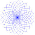
[edit | edit source]Already at the end of the 1970s, applications for the discrete spiral coordinate system were given in image analysis ( image registration ) . To represent an image in this coordinate system rather than in Cartesian coordinates, gives computational advantages when rotating or zooming in an image. Also, the photo receptors in the retina in the human eye are distributed in a way that has big similarities with the spiral coordinate system.[11] It can also be found in the Mandelbrot fractal (see picture to the right).
Log-polar coordinates can also be used to construct fast methods for the Radon transform and its inverse.[12]
Discrete geometry
[edit | edit source]-
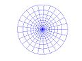 Discrete coordinate system in a circular disc given by log-polar coordinates (n = 25)
 -
 Discrete coordinate system in a circular disc that can easily be expressed in log-polar coordinates (n = 25)
 -
 Part of a Mandelbrot fractal showing spiral behaviour


In order to solve a PDE numerically in a domain, a discrete coordinate system must be introduced in this domain. If the domain has rotational symmetry and you want a grid consisting of rectangles, polar coordinates are a poor choice, since in the center of the circle it gives rise to triangles rather than rectangles.
However, this can be remedied by introducing log-polar coordinates in the following way:
- Divide the plane into a grid of squares with side length 2/n, where n is a positive integer
- Use the complex exponential function to create a log-polar grid in the plane. The left half-plane is then mapped onto the unit disc, with the number of radii equal to n. It can be even more advantageous to instead map the diagonals in these squares, which gives a discrete coordinate system in the unit disc consisting of spirals, see the figure to the right.

screen or image or device coordinate
[edit | edit source]- The coordinate values in an image are always positive[13]
- The origin = point 90,0) is located at the upper left corner of the screen
- The coordinates are integer values
- the coordinate system on the screen is left-handed, i.e. the x coordinate increases from left to right and the y coordinate increases from top to bottom.
Raster 2D graphic

world coordinate
[edit | edit source]// from screen to world coordinate ; linear mapping
// uses global cons
double GiveZx (int ix)
{
return (ZxMin + ix * PixelWidth);
}
// uses globaal cons
double GiveZy (int iy)
{
return (ZyMax - iy * PixelHeight);
} // reverse y axis
complex double GiveZ (int ix, int iy)
{
double Zx = GiveZx (ix);
double Zy = GiveZy (iy);
return Zx + Zy * I;
}
  // modified code using center and radius to scan the plane
  int height = 720;
  int width = 1280;
  double dWidth;
  double dRadius = 1.5;
  double complex center= -0.75*I;
  double complex c;
  int i,j;

  double width2; // = width/2.0
  double height2; // = height/2.0

  width2 = width /2.0;
  height2 = height/2.0;

complex double coordinate(int i, int j, int width, int height, complex double center, double radius) {
  double x = (i - width /2.0) / (height/2.0);
  double y = (j - height/2.0) / (height/2.0);
  complex double c = center + radius * (x - I * y);
  return c;
}

for ( j = 0; j < height; ++j) {
    for ( i = 0; i < width; ++i) {
      c = coordinate(i, j, width, height, center, dRadius);
      // do smth
       }
     }
or simply :
 double pixel_spacing = radius / (height / 2.0);
 complex double c = center + pixel_spacing * (x-width/2.0 + I * (y-height/2.0));
coordinate transformations
[edit | edit source]See also:
There are often many different possible coordinate systems for describing geometrical figures. The relationship between different systems is described by coordinate transformations, which give formulas for the coordinates in one system in terms of the coordinates in another system. For example, in the plane, if Cartesian coordinates (x, y) and polar coordinates (r, θ) have the same origin, and the polar axis is the positive x axis, then the coordinate transformation from polar to Cartesian coordinates is given by x = r cosθ and y = r sinθ.
With every bijection from the space to itself two coordinate transformations can be associated:
- Such that the new coordinates of the image of each point are the same as the old coordinates of the original point (the formulas for the mapping are the inverse of those for the coordinate transformation)
- Such that the old coordinates of the image of each point are the same as the new coordinates of the original point (the formulas for the mapping are the same as those for the coordinate transformation)
For example, in 1D, if the mapping is a translation of 3 to the right, the first moves the origin from 0 to 3, so that the coordinate of each point becomes 3 less, while the second moves the origin from 0 to −3, so that the coordinate of each point becomes 3 more. This is a list of some of the most commonly used coordinate transformations.
2-dimensional
[edit | edit source]Let (x, y) be the standard Cartesian coordinates, and (r, θ) the standard polar coordinates.
To Cartesian coordinates
[edit | edit source]From polar coordinates
[edit | edit source]![{\displaystyle {\begin{aligned}x&=r\cos \theta \\y&=r\sin \theta \\[5pt]{\frac {\partial (x,y)}{\partial (r,\theta )}}&={\begin{bmatrix}\cos \theta &-r\sin \theta \\\sin \theta &r\cos \theta \end{bmatrix}}\\[5pt]{\text{Jacobian}}=\det {\frac {\partial (x,y)}{\partial (r,\theta )}}&=r\end{aligned}}}](https://wikimedia.org/api/rest_v1/media/math/render/svg/6e812d8ce26cec97482d277c012e638ee182d298)
From log-polar coordinates
[edit | edit source]The formulas for transformation from Cartesian coordinates to log-polar coordinates are given by

and the formulas for transformation from log-polar to Cartesian coordinates are

By using complex numbers (x, y) = x + iy, the latter transformation can be written as

i.e. the complex exponential function.
From this follows that basic equations in harmonic and complex analysis will have the same simple form as in Cartesian coordinates. This is not the case for polar coordinates.

By using complex numbers , the transformation can be written as

That is, it is given by the complex exponential function.
From bipolar coordinates
[edit | edit source]
From 2-center bipolar coordinates
[edit | edit source]
From Cesàro equation
[edit | edit source]![{\displaystyle {\begin{aligned}x&=\int \cos \left[\int \kappa (s)\,ds\right]ds\\y&=\int \sin \left[\int \kappa (s)\,ds\right]ds\end{aligned}}}](https://wikimedia.org/api/rest_v1/media/math/render/svg/0cf415cca15fe7faf409efdfa8323225993978f8)
To polar coordinates
[edit | edit source]From Cartesian coordinates
[edit | edit source]
Note: solving for returns the resultant angle in the first quadrant (). To find , one must refer to the original Cartesian coordinate, determine the quadrant in which lies (for example, (3,−3) [Cartesian] lies in QIV), then use the following to solve for :


- For in QI:
- For in QII:
- For in QIII:
- For in QIV:


The value for must be solved for in this manner because for all values of , is only defined for , and is periodic (with period ). This means that the inverse function will only give values in the domain of the function, but restricted to a single period. Hence, the range of the inverse function is only half a full circle.


Note that one can also use

From 2-center bipolar coordinates
[edit | edit source]![{\displaystyle {\begin{aligned}r&={\sqrt {\frac {r_{1}^{2}+r_{2}^{2}-2c^{2}}{2}}}\\\theta &=\arctan \left[{\sqrt {{\frac {8c^{2}(r_{1}^{2}+r_{2}^{2}-2c^{2})}{r_{1}^{2}-r_{2}^{2}}}-1}}\right]\end{aligned}}}](https://wikimedia.org/api/rest_v1/media/math/render/svg/40fd7b0ef6f1fea0e4467981685d16feb513186d)
Where 2c is the distance between the poles.
To log-polar coordinates from Cartesian coordinates
[edit | edit source]
Arc-length and curvature
[edit | edit source]In Cartesian coordinates
[edit | edit source]
In polar coordinates
[edit | edit source]
3-dimensional
[edit | edit source]Let (x, y, z) be the standard Cartesian coordinates, and (ρ, θ, φ) the spherical coordinates, with θ the angle measured away from the +Z axis (as [1], see conventions in spherical coordinates). As φ has a range of 360° the same considerations as in polar (2 dimensional) coordinates apply whenever an arctangent of it is taken. θ has a range of 180°, running from 0° to 180°, and does not pose any problem when calculated from an arccosine, but beware for an arctangent.
If, in the alternative definition, θ is chosen to run from −90° to +90°, in opposite direction of the earlier definition, it can be found uniquely from an arcsine, but beware of an arccotangent. In this case in all formulas below all arguments in θ should have sine and cosine exchanged, and as derivative also a plus and minus exchanged.
All divisions by zero result in special cases of being directions along one of the main axes and are in practice most easily solved by observation.
To Cartesian coordinates
[edit | edit source]From spherical coordinates
[edit | edit source]
So for the volume element:

From cylindrical coordinates
[edit | edit source]
So for the volume element:

To spherical coordinates
[edit | edit source]From Cartesian coordinates
[edit | edit source]
See also the article on atan2 for how to elegantly handle some edge cases.
So for the element:

From cylindrical coordinates
[edit | edit source]
To cylindrical coordinates
[edit | edit source]From Cartesian coordinates
[edit | edit source]

From spherical coordinates
[edit | edit source]
Arc-length, curvature and torsion from Cartesian coordinates
[edit | edit source]![{\displaystyle {\begin{aligned}s&=\int _{0}^{t}{\sqrt {{x'}^{2}+{y'}^{2}+{z'}^{2}}}\,dt\\[3pt]\kappa &={\frac {\sqrt {(z''y'-y''z')^{2}+(x''z'-z''x')^{2}+(y''x'-x''y')^{2}}}{({x'}^{2}+{y'}^{2}+{z'}^{2})^{\frac {3}{2}}}}\\[3pt]\tau &={\frac {x'''(y'z''-y''z')+y'''(x''z'-x'z'')+z'''(x'y''-x''y')}{{(x'y''-x''y')}^{2}+{(x''z'-x'z'')}^{2}+{(y'z''-y''z')}^{2}}}\end{aligned}}}](https://wikimedia.org/api/rest_v1/media/math/render/svg/439b196b830ab79231f87b27a17af5ed4cf5f4e4)
implementations
[edit | edit source]wgpu
[edit | edit source]wgpu uses the coordinate systems of D3D and Metal:[14]
- Render: center is 0, and radius is 1, so right upper is (1,1) and left lower point is ( -1,-1)
- Texture: 0 is left upper point, right upper is (1,0), left lower is (0,1)
CSS box model for HTML
[edit | edit source]- user coordinate system
- local coordinate system
- transformation matrix
HTML canvas’ coordinate system [15]
- s a two-dimensional grid
- x increases from left to right: from x=0 (far left) to x=+960 (far right)
- y decreases from bottom to top: goes from y=+720 (bottom) to y=0 (top).
- The origin = 0,0 coordinate is in the top left ( The upper-left corner of the canvas )
OpenGL
[edit | edit source]-
 The three fundamental steps of a graphics pipeline
 -
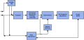 Pipeline OpenGL
 -
 the geometry steps in a graphics pipeline
 -
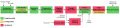 3D graphics rendering pipeline

![[1]](https://commons.wikimedia.org/wiki/File:3D_Spherical.svg)
5 different coordinate systems in OpenGL:[16]
- Local or Object
- World
- View or Eye
- Clip
- Screen
OpenGl :
- "OpenGL is right handed in object space and world space, But in window space (aka screen space) we are suddenly left handed"[17]
- the transformation pipeline: local coordinates -> world coordinates -> view coordinates -> clip coordinates -> screen coordinates[18] "Each coordinate system serves a purpose for one or more OpenGL features"[19]
- using
OpenCV
[edit | edit source]- The origin of the OpenCV image coordinate system is at the top-left corner of the image
SVG
[edit | edit source]SVG coordinate systems
- The default coordinate system in SVG is much the same as in HTML
- canvas the space or area where all SVG elements are drawn[22]
- viewport defines a drawing region characterized by size (width, height), and an origin, measured in abstract user units. Term SVG viewport is distinct from the "viewport" term used in CSS
- viewBox[23]
p5.js library
[edit | edit source]2D coordinate system[24]
- canvas
- origin ( 0,0) it's location
See also
[edit | edit source]
References
[edit | edit source]- ↑ Coordinate Systems by Dr. John T. Bell
- ↑ wikipedia : Coordinate_system
- ↑ computergraphics stackexchange question: what-is-the-difference-between-world-coordinate-viewing-coordinate-and-device-c
- ↑ javatpoint : computer-graphics-window
- ↑ A Pixel Is Not A Little Square by Alvy Ray Smith
- ↑ How to convert world to screen coordinates and vice versa
- ↑ How to transform 2D world to screen coordinates OpenGL
- ↑ An interactive guide to homogeneous coordinates by Words and Buttons Online — a collection of interactive
- ↑ Homogeneous Coordinates by Yasen Hu
- ↑ Image Registration Using Log Polar Transform and Phase Correlation to Recover Higher Scale JIGNESH NATVARLAL SARVAIYA, Dr. Suprava Patnaik, Kajal Kothari JPRR Vol 7, No 1 (2012); doi:10.13176/11.355
- ↑ Weiman, Chaikin, Logarithmic Spiral Grids for Image Processing and Display, Computer Graphics and Image Processing 11, 197–226 (1979).
- ↑ Andersson, Fredrik, Fast Inversion of the Radon Transform Using Log-polar Coordinates and Partial Back-Projections, SIAM J. Appl. Math. 65, 818–837 (2005).
- ↑ ronny restrepo : point cloud coordinates
- ↑ raphlinus: wgpu
- ↑ w3schools : canvas coordinates
- ↑ learnopengl : Coordinate-Systems
- ↑ stackoverflow question: is-opengl-coordinate-system-left-handed-or-right-handed
- ↑ learnopengl : Coordinate-Systems
- ↑ The OpenGL transformation pipeline by Paul Martz
- ↑ Homogeneous Coordinates by Song Ho Ahn
- ↑ Python & OpenGL for Scientific Visualization Copyright (c) 2018 - Nicolas P. Rougier
- ↑ SVG Coordinate Systems and Units by ASPOSE
- ↑ svg-coordinate-systems by Sara Soueidan
- ↑ 2D coordinate systems University of London, Goldsmiths, University of London