Fractals/scanning
Scanning, sampling
Sampling
- process of getting a finite number of values from a function, map, image.[1][2]
- In statistics, quality assurance, and survey methodology, sampling is the selection of a subset (a statistical sample) of individuals from within a statistical population to estimate characteristics of the whole population. Statisticians attempt to collect samples that are representative of the population in question. Sampling has lower costs and faster data collection than measuring the entire population and can provide insights in cases where it is infeasible to measure an entire population.
Criteria for classifications:
- number of passes ( single pass, multiple pass)
- grid ( regular = uniform / irregular or adaptive )
- random ( stochastic)/ not-random
- with or without decomposition
Sampling types by range
- point-sampling = Point-sampling method. A seed is a defined, rationally complex number which represents a pixel = pixel center. Note that one can find infinitely many points inside one pixel, and many of such point can have different color/ behaviour then the pixel center.
- Spatial sampling ( what happens between samples ? ) : a manually-defined homogeneous grid = uniform sampling
- 1 pixel approximation = image shows "the set of points in the plane whose distance to the filled Julia set is at most the diameter of a pixel"[3]
Sampling by adaptation
- regular, uniform ( non-adaptive) sampling
- adaptive ( non-uniform)sampling = Adaptive Mesh Refinement (AMR)
- Detail Enhancement Based on Local Fractal Analysis of Gradient: The key concept of fractal-based image model is the fractal dimension is capable of representing intrinsic structural information of image robustly.[6][7]
- a quadtree decomposition of the complex plane with adaptive refinement gives adaptive approximation
Types
[edit | edit source]- standard scanning: rendering the whole image (in full resolution) in one step
- fractint Drawing_Methods
- circular rendering on each successive refinement step
Steps:
- preview
- final render
Types by transformation or plane type ( parameter or dynamic)
- scaning the standard c plane
- scanning the exponential plane
standard
[edit | edit source]Scan the plane :
- all pixels ( plane is scanned pixel by pixel ) in one pass
- the same pixel size ( regular, uniform grid )
It depends also on the plane description
int SetPlane(complex double center, double radius, double a_ratio){

	ZxMin = creal(center) - radius*a_ratio;
	ZxMax = creal(center) + radius*a_ratio;	//0.75;
	ZyMin = cimag(center) - radius;	// inv
	ZyMax = cimag(center) + radius;	//0.7;
    double PixelWidth = (ZxMax-ZxMin)/iWidth;
    double PixelHeight = (ZyMax-ZyMin)/iHeight; // pixel_size = PixelWidth = PixelHeight
	return 0;

}
corners
[edit | edit source]Here in Lisp
; common lisp. Here float values can be used,  there is no mapping
(loop for y from -1.5 to 1.5 by 0.1 do
      (loop for x from -2.5 to 0.5 by 0.05 do
            (princ (code-char 42))) ; print char
      (format t "~%")) ; new line
and in C
/* c */
/* screen coordinate = coordinate of pixels */
int iX, iY,
iXmin=0, iXmax=1000,
iYmin=0, iYmax=1000,
iWidth=iXmax-iXmin+1,
iHeight=iYmax-iYmin+1;

/* world ( double) coordinate = parameter plane*/
const double ZxMin=-5;
const double ZxMax=5;
const double ZyMin=-5;
const double ZyMax=5;

/* */
double PixelWidth=(ZxMax-ZxMin)/iWidth;
double PixelHeight=(ZyMax-ZyMin)/iHeight;
double Zx, Zy,    /* Z=Zx+Zy*i   */
       Z0x, Z0y,  /* Z0 = Z0x + Z0y*i */

 for(iY=0;iY<iYmax;++iY)
      { Z0y=ZyMin + iY*PixelHeight; /* mapping from screen to world; reverse Y  axis */
        if (fabs(Z0y)<PixelHeight/2) Z0y=0.0; /* Zy = 0 is a special value  */
        for(iX=0;iX<iXmax;++iX)
         {    /* initial value of orbit Z0 */
           Z0x=ZxMin + iX*PixelWidth;
          }
      }
Normal grid-scan plotting by Robert Munafo[10]
  /* Plot a single pixel, row i and column j

   NOTE:
     itmax is the maximum number of Mandelbrot iterations
     min_r is the real coordinate of the left edge of the image
     max_i is the imaginary coordinate of the top of the image
     px_spacing = pixel size  is the width of the image (in real coordinates) divided by the number of pixels in a row
     image aspect ratio = 1:1
  */
  void pixel_53(int i, int j, int itmax)
  {
    double cr, ci;

    ci = max_i - ((double) i) * px_spacing;
    cr = min_r + ((double) j) * px_spacing;
    evaluate_and_plot(cr, ci, itmax, i, j);
  }
radius
[edit | edit source] // modified code using center and radius to scan the plane
int height = 720;
int width = 1280;
double dWidth;
double dRadius = 1.5;
double complex center= -0.75*I;
double complex c;
int i,j;
double width2; // = width/2.0
double height2; // = height/2.0
width2 = width /2.0;
height2 = height/2.0;
complex double coordinate(int i, int j, int width, int height, complex double center, double radius) {
double x = (i - width /2.0) / (height/2.0);
double y = (j - height/2.0) / (height/2.0);
complex double c = center + radius * (x - I * y);
return c;
}
for ( j = 0; j < height; ++j) {
for ( i = 0; i < width; ++i) {
c = coordinate(i, j, width, height, center, dRadius);
// do smth
}
}
another version
int main()
{
  int aa = 4;
  int w = 800 * aa;
  int h = 800 * aa;

  #pragma omp parallel for schedule(static, 1)
  for (int j = 0; j < h; ++j)
  {
    double y = (h/2 - (j + 0.5)) / (h/2) * r;
    for (int i = 0; i < w; ++i)
    {
      double x = (i + 0.5 - w/2) / (h/2) * r;
      double _Complex c = x + I * y;
      // proceed
    }
  }

  return 0;
}
plane decomposition
[edit | edit source]quadtree
[edit | edit source]Quadtree types
- Region quadtree
- point quadtree
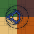
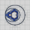
- distance_estimation, Koebe 1/4-theorem by Claude Heiland-Allen
- fast-mandelbrot-set-by-quadtree by Mandrian
- The Mariani-Silver Algorithm for Drawing the Mandelbrot Set by Rico Mariani
- Mariani/Silver Algorithm from the Mandelbrot Set Glossary and Encyclopedia, by Robert Munafo, (c) 1987-2022.
- openprocessing : Quad-tree by Naoki Tsutae
-
-

-
-
 Mandelbrot multithreaded
 -
-
 iteration visualization
 -


// Quad-tree by Naoki Tsutae in Processing
// https://openprocessing.org/sketch/1769288
quadTree = (x, y, size) => {
 if (size < minRectSize) return;
 const n = noise((x + posx) * 0.001, (y + posy) * 0.001, variation);
 if (abs(n - 0.45) > size / maxRectSize) {
   rect(x, y, size);
 } else {
   size /= 2;
   const d = size / 2;
   quadTree(x + d, y + d, size);
   quadTree(x + d, y - d, size);
   quadTree(x - d, y + d, size);
   quadTree(x - d, y - d, size);
 }
};
Region quadtree
[edit | edit source]The region quadtree represents a partition of space in two dimensions by decomposing the region into four equal quadrants, subquadrants, and so on with each leaf node containing data corresponding to a specific subregion. Each node in the tree either has
- exactly four children
- or has no children (a leaf node).
The height of quadtrees that follow this decomposition strategy (i.e. subdividing subquadrants as long as there is interesting data in the subquadrant for which more refinement is desired) is sensitive to and dependent on the spatial distribution of interesting areas in the space being decomposed. The region quadtree is a type of trie.
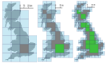
A region quadtree with a depth of n may be used to represent an image consisting of 2n × 2n pixels, where each pixel value is 0 or 1. The root node represents the entire image region. If the pixels in any region are not entirely 0s or 1s, it is subdivided. In this application, each leaf node represents a block of pixels that are all 0s or all 1s. Note the potential savings in terms of space when these trees are used for storing images; images often have many regions of considerable size that have the same colour value throughout. Rather than store a big 2-D array of every pixel in the image, a quadtree can capture the same information potentially many divisive levels higher than the pixel-resolution sized cells that we would otherwise require. The tree resolution and overall size is bounded by the pixel and image sizes.
A region quadtree may also be used as a variable resolution representation of a data field. For example, the temperatures in an area may be stored as a quadtree, with each leaf node storing the average temperature over the subregion it represents.
Once b [the exterior distance estimate for c] is found, by the Koebe 1/4-theorem, we know there's no point of the Mandelbrot set with distance from c smaller than b/4.
// code in Haskell by Claude Heiland-Allen https://mathr.co.uk/blog/2010-10-30_distance_estimation.html
exterior :: Square -> Bool
exterior s@(Square a b c d) = fromMaybe False $ do
  lb <- distance a
  lt <- distance b
  rb <- distance c
  rt <- distance d
  let k = 4 * sqrt 2 * size s
  return $ and
    [ lb + rb > k
    , lt + rt > k
    , lb + lt > k
    , rb + rt > k
    ]
Antialiasing and supersampling
[edit | edit source]
Supersampling or supersampling anti-aliasing (SSAA) is a spatial anti-aliasing method, i.e. a method used to remove aliasing (jagged and pixelated edges, colloquially known as "jaggies") from images rendered in computer games or other computer programs that generate imagery. Aliasing occurs because unlike real-world objects, which have continuous smooth curves and lines, a computer screen shows the viewer a large number of small squares. These pixels all have the same size, and each one has a single color. A line can only be shown as a collection of pixels, and therefore appears jagged unless it is perfectly horizontal or vertical. The aim of supersampling is to reduce this effect. Color samples are taken at several instances inside the pixel (not just at the center as normal), and an average color value is calculated. This is achieved by rendering the image at a much higher resolution than the one being displayed, then shrinking it to the desired size, using the extra pixels for calculation. The result is a downsampled image with smoother transitions from one line of pixels to another along the edges of objects.
The number of samples determines the quality of the output.
- TechInfo -AntiAliasing by Michael Condron
- Fract (Lisp code) by Yannick Gingras
- Spatial anti aliasing at wikipedia[11]
- fractalforums discussion: Antialiasing fractals - how best to do it?[12]
- Supersampling
-
 example of supersampled image
 -
 Cpp code of supersampling
 -
 Aliased chessboard - image and c src code


Supersampling, other names:
- antigrain geometry
- Supersampling (downsampling)[13][14]
- downsizing
- downscaling[15]
- subpixel accuracy
Computational cost and adaptive supersampling
[edit | edit source]Supersampling is computationally expensive because it requires much greater video card memory and memory bandwidth, since the amount of buffer used is several times larger.[16] A way around this problem is to use a technique known as adaptive supersampling, where only pixels at the edges of objects are supersampled.
Initially only a few samples are taken within each pixel. If these values are very similar, only these samples are used to determine the color. If not, more are used. The result of this method is that a higher number of samples are calculated only where necessary, thus improving performance.
Types
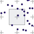
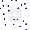
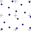
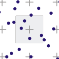
[edit | edit source]When taking samples within a pixel, the sample positions have to be determined in some way. Although the number of ways in which this can be done is infinite, there are a few ways which are commonly used.[16][17]
-
 Grid algorithm in uniform distribution
 -
 Rotated grid algorithm (with 2x times the sample density)
 -
 Random algorithm
 -
 Jitter algorithm
 -
 Poisson disc algorithm
 -
 Quasi-Monte Carlo method algorithm
 -
 N-Rooks
 -
 RGSS
RGSS -
 High-resolution antialiasing (HRAA), Quincunx
 -
 Flipquad
 -
 Fliptri


Grid
[edit | edit source]The simplest algorithm. The pixel is split into several sub-pixels, and a sample is taken from the center of each. It is fast and easy to implement. Although, due to the regular nature of sampling, aliasing can still occur if a low number of sub-pixels is used.
Random
[edit | edit source]Also known as stochastic sampling, it avoids the regularity of grid supersampling. However, due to the irregularity of the pattern, samples end up being unnecessary in some areas of the pixel and lacking in others.[18]
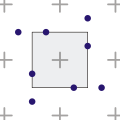
Poisson disk
[edit | edit source]-
 Point samples generated using Poisson disk sampling, and graphical representation of the minimum inter-point distance

The poisson disk sampling algorithm [19] places the samples randomly, but then checks that any two are not too close. The end result is an even but random distribution of samples. However, the computational time required for this algorithm is too great to justify its use in real-time rendering, unless the sampling itself is computationally expensive compared to the positioning of the sample points or the sample points are not repositioned for every single pixel.[18]
Poisson-disk sampling (blue noise) is the best sampling pattern. It maximizes the uniformity of the samples in addition to the randomness of their placement, which gets you the most bang for your buck with respect to the contribution of each sample. quaz0r on FF
Links
Jittered
[edit | edit source]A modification of the grid algorithm to approximate the Poisson disk. A pixel is split into several sub-pixels, but a sample is not taken from the center of each, but from a random point within the sub-pixel. Congregation can still occur, but to a lesser degree.[18] Jitter is also recommended to avoid Moiré artifacts.
Rotated grid
[edit | edit source]A 2×2 grid layout is used but the sample pattern is rotated to avoid samples aligning on the horizontal or vertical axis, greatly improving antialiasing quality for the most commonly encountered cases. For an optimal pattern, the rotation angle is arctan (12) (about 26.6°) and the square is stretched by a factor of [20] [citation needed]

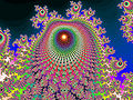
An example of an image with extreme pseudo-random aliasing
[edit | edit source]Because fractals have unlimited detail and no noise other than arithmetic round-off error, they illustrate aliasing more clearly than do photographs or other measured data. The escape times, which are converted to colours at the exact centres of the pixels, go to infinity at the border of the set, so colours from centres near borders are unpredictable, due to aliasing. This example has edges in about half of its pixels, so it shows much aliasing. The first image is uploaded at its original sampling rate. (Since most modern software anti-aliases, one may have to download the full-size version to see all of the aliasing.) The second image is calculated at five times the sampling rate and down-sampled with anti-aliasing. Assuming that one would really like something like the average colour over each pixel, this one is getting closer. It is clearly more orderly than the first.
In order to properly compare these images, viewing them at full-scale is necessary.
-
 1. As calculated with the program "MandelZot"
 -
 2. Anti-aliased by blurring and down-sampling by a factor of five
 -
 3. Edge points interpolated, then anti-aliased and down-sampled
 -
 4. An enhancement of the points removed from the previous image
 -
 5. Down-sampled again, without anti-aliasing


It happens that, in this case, there is additional information that can be used. By re-calculating with a "distance estimator" algorithm, points were identified that are very close to the edge of the set, so that unusually fine detail is aliased in from the rapidly changing escape times near the edge of the set. The colours derived from these calculated points have been identified as unusually unrepresentative of their pixels. The set changes more rapidly there, so a single point sample is less representative of the whole pixel. Those points were replaced, in the third image, by interpolating the points around them. This reduces the noisiness of the image but has the side effect of brightening the colours. So this image is not exactly the same that would be obtained with an even larger set of calculated points. To show what was discarded, the rejected points, blended into a grey background, are shown in the fourth image.
Finally, "Budding Turbines" is so regular that systematic (Moiré) aliasing can clearly be seen near the main "turbine axis" when it is downsized by taking the nearest pixel. The aliasing in the first image appears random because it comes from all levels of detail, below the pixel size. When the lower level aliasing is suppressed, to make the third image and then that is down-sampled once more, without anti-aliasing, to make the fifth image, the order on the scale of the third image appears as systematic aliasing in the fifth image.
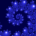
Pure down-sampling of an image has the following effect (viewing at full-scale is recommended):
-
 1) A picture of a particular spiral feature of the Mandelbrot set
 -
 2) 4 samples per pixel
 -
 3) 25 samples per pixel
 -
 4) 400 samples per pixel


code
[edit | edit source]- Cpp code by User Geek3
 // subpixels finished -> make arithmetic mean
 char pixel[3];
 for (int c = 0; c < 3; c++)
   pixel[c] = (int)(255.0 * sum[c] / (subpix * subpix)  + 0.5);
 fwrite(pixel, 1, 3, image_file);
 //pixel finished
- command line version of Aptus (python and c code) by Ned Batchelder[21] (see aptuscmd.py) is using a high-quality downsampling filter thru PIL function resize[22]
- Java code by Josef Jelinek:[23] supersampling with grid algorithm, computes 4 new points (corners), resulting color is an average of each color component:
 //Created by Josef Jelinek
 // http://java.rubikscube.info/
 Color c0 = color(dx, dy); // color of central point
 // computation of 4 new points for antialiasing
 if (antialias) { // computes 4 new points (corners)
   Color c1 = color(dx - 0.25 * r, dy - 0.25 * r);
   Color c2 = color(dx + 0.25 * r, dy - 0.25 * r);
   Color c3 = color(dx + 0.25 * r, dy + 0.25 * r);
   Color c4 = color(dx - 0.25 * r, dy + 0.25 * r);
  // resulting color; each component of color is an avarage of 5 values (central point and 4 corners)
   int red = (c0.getRed() + c1.getRed() + c2.getRed() + c3.getRed() + c4.getRed()) / 5;
   int green = (c0.getGreen() + c1.getGreen() + c2.getGreen() + c3.getGreen() + c4.getGreen()) / 5;
   int blue = (c0.getBlue() + c1.getBlue() + c2.getBlue() + c3.getBlue() + c4.getBlue()) / 5;
   color = new Color(red, green, blue);
 }
- one can make big image (like 10 000 x 10 000) and convert/resize it (downsize). For example using ImageMagick:
convert big.ppm -resize 2000x2000 m.png
downsampling and interpolating is essentially compression, low frequency components, ie:
- slow changing colours that change slower than half sampling freq, will get preserved
- the high frequency detail will be lost
Interval arithmetic
[edit | edit source]- adaptive algorithms for generating guaranted images of Julia sets[24][25][26][27][28][29]
- True Shape Algorithm ( TSA)
How do I optimize searching for the nearest point ?
[edit | edit source]See also
[edit | edit source]- Tessellation is the process of partitioning space into a set of smaller polygons
- 2D grid types
- commons:Category:Mesh in computer graphics
- sampling and the image noise - dither to more accurately display graphics containing a greater range of colors than the display hardware is capable of showing
- Fractint Drawing Methods[30]
- Fratal Witchcraft drawing methods by Steven Stoft[31]
- AlmondBread algorithms [32]
- rugh set method [33]
- cell mapping based on interval arithmetic with label propagation in graphs to avoid function iteration and rounding errors [34]
- "We combine cell mapping based on interval arithmetic with label propagation in graphs to avoid function iteration and rounding errors." - Luiz Henrique de Figueiredo et al.[35][36]
- using exterior distance estimates[37] and Koebe quarter theorem
- usung symmetry
References
[edit | edit source]- ↑ textures-and-sampling from University of Tartu:
- ↑ fractalforums.org : sampling
- ↑ "Images of Julia sets that you can trust" by Luiz-Henrique de Figueiredo, Diego Nehab, Jofge Stolfi, Joao Batista Oliveira- IEE 2015
- ↑ Supersampling in wikipedia
- ↑ Sub-pixel resolution in wikipedia
- ↑ researchgate : Single Image Super-resolution With Detail Enhancement Based on Local Fractal Analysis of Gradient by HONGTENG Xu, Xiaokang Yang, Guangtao Zhai
- ↑ Hongteng Xu: Fractal-based-image-processing
- ↑ wolfram mathematica: AdaptiveSamplingOfSurfaces
- ↑ Adaptive Sampling, Plotting Math Curve By Xah Lee. Date: 2016-05-01. Last updated: 2016-05-07.
- ↑ From the Mandelbrot Set Glossary and Encyclopedia, by Robert Munafo, (c) 1987-2020.Exponential Map by Robert P. Munafo, 2010 Dec 5.
- ↑ Spatial anti aliasing at wikipedia
- ↑ fractalforums discussion: Antialiasing fractals - how best to do it?
- ↑ Supersampling at wikipedia
- ↑ ImageMagick v6 Examples -- Resampling Filters
- ↑ What is the best image downscaling algorithm (quality-wise)?
- ↑ a b "Anti-aliasing techniques comparison". sapphirenation.net. 2016-11-29. Retrieved 2020-04-19.
Generally speaking, SSAA provides exceptional image quality, but the performance hit is major here because the scene is rendered at a very high resolution.
- ↑ "What is supersampling?". everything2.com. 2004-05-20. Retrieved 2020-04-19.
- ↑ a b c Allen Sherrod (2008). Game Graphic Programming. Charles River Media. p. 336. ISBN 978-1584505167.
- ↑ Cook, R. L. (1986). "Stochastic sampling in computer graphics". ACM Transactions on Graphics. 5 (1): 51–72. doi:10.1145/7529.8927. S2CID 8551941.
- ↑ "Super-sampling Anti-aliasing Analyzed" (PDF). Beyond3D.com. Retrieved 2020-04-19.
- ↑ Aptus (python and c code) by Ned Batchelder
- ↑ Pil function resize
- ↑ Java code by Josef Jelinek
- ↑ Images of Julia sets that you can trust Luiz Henrique de Figueiredo
- ↑ ON THE NUMERICAL CONSTRUCTION OF HYPERBOLIC STRUCTURES FOR COMPLEX DYNAMICAL SYSTEMS by Jennifer Suzanne Lynch Hruska
- ↑ "Images of Julia sets that you can trust" by Luiz Henrique de Figueiredo and Joao Batista Oliveira
- ↑ adaptive algorithms for generating guaranteed images of Julia sets by Luiz Henrique de Figueiredo
- ↑ Drawing Fractals With Interval Arithmetic - Part 1 by Dr Rupert Rawnsley
- ↑ Drawing Fractals With Interval Arithmetic - Part 2 by Dr Rupert Rawnsley
- ↑ Fractint Drawing Methods
- ↑ Synchronous-Orbit Algorithm by R Munafo
- ↑ The Almond BreadHomepage by Michael R. Ganss
- ↑ Rough Mandelbrot Sets by Neural Outlet.. posted on 23/11/2014
- ↑ Images of Julia sets that you can trust by Luiz Henrique de Figueiredo, Diego Nehab, Jorge Stolfi, and Joao Batista Oliveira
- ↑ RIGOROUS BOUNDS FOR POLYNOMIAL JULIA SETS by Luiz Henrique de Figueiredo
- ↑ Images of Julia sets that you can trust by LUIZ HENRIQUE DE FIGUEIREDO and DIEGO NEHAB
- ↑ Distance estimation by Claude Heiland-Allen