Control Systems/Print version
| This is the print version of Control Systems You won't see this message or any elements not part of the book's content when you print or preview this page. |

The Wikibook of automatic
And Control Systems Engineering
With
Classical and Modern Techniques
And
Advanced Concepts
Preface
This book will discuss the topic of Control Systems, which is an interdisciplinary engineering topic. Methods considered here will consist of both "Classical" control methods, and "Modern" control methods. Also, discretely sampled systems (digital/computer systems) will be considered in parallel with the more common analog methods. This book will not focus on any single engineering discipline (electrical, mechanical, chemical, etc.), although readers should have a solid foundation in the fundamentals of at least one discipline.
This book will require prior knowledge of linear algebra, integral and differential calculus, and at least some exposure to ordinary differential equations. In addition, a prior knowledge of integral transforms, specifically the Laplace and Z transforms will be very beneficial. Also, prior knowledge of the Fourier Transform will shed more light on certain subjects. Wikibooks with information on calculus topics or transformation topics required for this book will be listed below:
Table of Contents
Table of Contents
Special Pages
| Print Version: | Full Print version () |
Warning: Print version is over 230 pages long as of 10 Feb, 2014. |
| PDF Version: | PDF Version | Warning: PDF version is over 5.4MB, as of 21 Jan, 2014. |
| Cover Page: | Cover Page | Cover Image |
| All Pages: | Page Listing | All Versions |
| Book Policy: | Policy | Local Manual of Style |
| Search This Book: | (links to an external site) |
Controls Introduction
Classical Control Methods
Modern Control Methods
- State-Space Equations
- Linear System Solutions
- Time-Variant System Solutions
- Digital State-Space
- Eigenvalues and Eigenvectors
- Standard Forms
- MIMO Systems
- Realizations
System Representation
Stability
- Stability
- State-Space Stability
- Discrete-Time Stability
- Routh-Hurwitz Criterion
- Jury's Test
- Root Locus
- Nyquist Stability Criterion
Controllers and Compensators
- Controllability and Observability
- System Specifications
- State Feedback
- Estimators and Observers
- Eigenvalue Assignment for MIMO Systems
- Controllers and Compensators
- Polynomial Design
Adaptive Control
Nonlinear Systems
Noisy Systems
Introduction to Digital Controls
- Digital Control Systems
- Discrete-Time Stability
- System Delays
- Sampled Data Systems
- Z Transform Mappings
Linear Matrix Inequalities in Control
Examples
Appendices
- Physical Models
- Transforms
- System Representations
- Matrix Operations
- Using MATLAB ®
- Using Octave
- Using Julia
- Using Scilab
- Using Python
Resources, Glossary, and License
Introduction to Control Systems
What are control systems? Why do we study them? How do we identify them? The chapters in this section should answer these questions and more.
Introduction
This Wikibook
This book was written at Wikibooks, a free online community where people write open-content textbooks. Any person with internet access is welcome to participate in the creation and improvement of this book. Because this book is continuously evolving, there are no finite "versions" or "editions" of this book. Permanent links to known good versions of the pages may be provided.
What are Control Systems?
The study and design of automatic Control Systems, a field known as control engineering, has become important in modern technical society. From devices as simple as a toaster or a toilet, to complex machines like space shuttles and power steering, control engineering is a part of our everyday life. This book introduces the field of control engineering and explores some of the more advanced topics in the field. Note, however, that control engineering is a very large field and this book serves only as a foundation of control engineering and an introduction to selected advanced topics in the field. Topics in this book are added at the discretion of the authors and represent the available expertise of our contributors.
Control systems are components that are added to other components to increase functionality or meet a set of design criteria. For example:
We have a particular electric motor that is supposed to turn at a rate of 40 RPM. To achieve this speed, we must supply 10 Volts to the motor terminals. However, with 10 volts supplied to the motor at rest, it takes 30 seconds for our motor to get up to speed. This is valuable time lost.
This simple example can be complex to both users and designers of the motor system. It may seem obvious that the motor should start at a higher voltage so that it accelerates faster. Then we can reduce the supply back down to 10 volts once it reaches ideal speed.
This is clearly a simplistic example but it illustrates an important point: we can add special "Controller units" to preexisting systems to improve performance and meet new system specifications.
Here are some formal definitions of terms used throughout this book:
- Control System
- A Control System is a device, or a collection of devices that manage the behavior of other devices. Some devices are not controllable. A control system is an interconnection of components connected or related in such a manner as to command, direct, or regulate itself or another system.
Control System is a conceptual framework for designing systems with capabilities of regulation and/or tracking to give a desired performance. For this there must be a set of signals measurable to know the performance, another set of signals measurable to influence the evolution of the system in time and a third set which is not measurable but disturb the evolution.
- Controller
- A controller is a control system that manages the behavior of another device or system (using Actuators). The controller is usually fed with some input signal from outside the system which commands the system to provide desired output. In a closed loop system, the signal is preprocessed with the sensor's signal from inside the system.
- Actuator
- An actuator is a device that takes in a signal form the controller and carries some action to affect the system accordingly.
- Compensator
- A compensator is a control system that regulates another system, usually by conditioning the input or the output to that system. Compensators are typically employed to correct a single design flaw with the intention of minimizing effects on other aspects of the design.
There are essentially two methods to approach the problem of designing a new control system: the Classical Approach and the Modern Approach.
Classical and Modern
Classical and Modern control methodologies are named in a misleading way, because the group of techniques called "Classical" were actually developed later than the techniques labeled "Modern". However, in terms of developing control systems, Modern methods have been used to great effect more recently, while the Classical methods have been gradually falling out of favor. Most recently, it has been shown that Classical and Modern methods can be combined to highlight their respective strengths and weaknesses.
Classical Methods, which this book will consider first, are methods involving the Laplace Transform domain. Physical systems are modeled in the so-called "time domain", where the response of a given system is a function of the various inputs, the previous system values, and time. As time progresses, the state of the system and its response change. However, time-domain models for systems are frequently modeled using high-order differential equations which can become impossibly difficult for humans to solve and some of which can even become impossible for modern computer systems to solve efficiently. To counteract this problem, integral transforms, such as the Laplace Transform and the Fourier Transform, can be employed to change an Ordinary Differential Equation (ODE) in the time domain into a regular algebraic polynomial in the transform domain. Once a given system has been converted into the transform domain it can be manipulated with greater ease and analyzed quickly by humans and computers alike.
Modern Control Methods, instead of changing domains to avoid the complexities of time-domain ODE mathematics, converts the differential equations into a system of lower-order time domain equations called State Equations, which can then be manipulated using techniques from linear algebra. This book will consider Modern Methods second.
A third distinction that is frequently made in the realm of control systems is to divide analog methods (classical and modern, described above) from digital methods. Digital Control Methods were designed to try and incorporate the emerging power of computer systems into previous control methodologies. A special transform, known as the Z-Transform, was developed that can adequately describe digital systems, but at the same time can be converted (with some effort) into the Laplace domain. Once in the Laplace domain, the digital system can be manipulated and analyzed in a very similar manner to Classical analog systems. For this reason, this book will not make a hard and fast distinction between Analog and Digital systems, and instead will attempt to study both paradigms in parallel.
Who is This Book For?
This book is intended to accompany a course of study in under-graduate and graduate engineering. As has been mentioned previously, this book is not focused on any particular discipline within engineering, however any person who wants to make use of this material should have some basic background in the Laplace transform (if not other transforms), calculus, etc. The material in this book may be used to accompany several semesters of study, depending on the program of your particular college or university. The study of control systems is generally a topic that is reserved for students in their 3rd or 4th year of a 4 year undergraduate program, because it requires so much previous information. Some of the more advanced topics may not be covered until later in a graduate program.
Many colleges and universities only offer one or two classes specifically about control systems at the undergraduate level. Some universities, however, do offer more than that, depending on how the material is broken up, and how much depth that is to be covered. Also, many institutions will offer a handful of graduate-level courses on the subject. This book will attempt to cover the topic of control systems from both a graduate and undergraduate level, with the advanced topics built on the basic topics in a way that is intuitive. As such, students should be able to begin reading this book in any place that seems an appropriate starting point, and should be able to finish reading where further information is no longer needed.
What are the Prerequisites?
Understanding of the material in this book will require a solid mathematical foundation. This book does not currently explain, nor will it ever try to fully explain most of the necessary mathematical tools used in this text. For that reason, the reader is expected to have read the following wikibooks, or have background knowledge comparable to them:
- Algebra
- Calculus
- The reader should have a good understanding of differentiation and integration. Partial differentiation, multiple integration, and functions of multiple variables will be used occasionally, but the students are not necessarily required to know those subjects well. These advanced calculus topics could better be treated as a co-requisite instead of a pre-requisite.
- Linear Algebra
- State-space system representation draws heavily on linear algebra techniques. Students should know how to operate on matrices. Students should understand basic matrix operations (addition, multiplication, determinant, inverse, transpose). Students would also benefit from a prior understanding of Eigenvalues and Eigenvectors, but those subjects are covered in this text.
- Ordinary Differential Equations
- All linear systems can be described by a linear ordinary differential equation. It is beneficial, therefore, for students to understand these equations. Much of this book describes methods to analyze these equations. Students should know what a differential equation is, and they should also know how to find the general solutions of first and second order ODEs.
- Engineering Analysis
- This book reinforces many of the advanced mathematical concepts used in the Engineering Analysis book, and we will refer to the relevant sections in the aforementioned text for further information on some subjects. This is essentially a math book, but with a focus on various engineering applications. It relies on a previous knowledge of the other math books in this list.
- Signals and Systems
- The Signals and Systems book will provide a basis in the field of systems theory, of which control systems is a subset. Readers who have not read the Signals and Systems book will be at a severe disadvantage when reading this book.
How is this Book Organized?
This book will be organized following a particular progression. First this book will discuss the basics of system theory, and it will offer a brief refresher on integral transforms. Section 2 will contain a brief primer on digital information, for students who are not necessarily familiar with them. This is done so that digital and analog signals can be considered in parallel throughout the rest of the book. Next, this book will introduce the state-space method of system description and control. After section 3, topics in the book will use state-space and transform methods interchangeably (and occasionally simultaneously). It is important, therefore, that these three chapters be well read and understood before venturing into the later parts of the book.
After the "basic" sections of the book, we will delve into specific methods of analyzing and designing control systems. First we will discuss Laplace-domain stability analysis techniques (Routh-Hurwitz, root-locus), and then frequency methods (Nyquist Criteria, Bode Plots). After the classical methods are discussed, this book will then discuss Modern methods of stability analysis. Finally, a number of advanced topics will be touched upon, depending on the knowledge level of the various contributors.
As the subject matter of this book expands, so too will the prerequisites. For instance, when this book is expanded to cover nonlinear systems, a basic background knowledge of nonlinear mathematics will be required.
Versions
This wikibook has been expanded to include multiple versions of its text, differentiated by the material covered, and the order in which the material is presented. Each different version is composed of the chapters of this book, included in a different order. This book covers a wide range of information, so if you don't need all the information that this book has to offer, perhaps one of the other versions would be right for you and your educational needs.
Each separate version has a table of contents outlining the different chapters that are included in that version. Also, each separate version comes complete with a printable version, and some even come with PDF versions as well.
Take a look at the All Versions Listing Page to find the version of the book that is right for you and your needs.
Differential Equations Review
Implicit in the study of control systems is the underlying use of differential equations. Even if they aren't visible on the surface, all of the continuous-time systems that we will be looking at are described in the time domain by ordinary differential equations (ODE), some of which are relatively high-order.
Let's review some differential equation basics. Consider the topic of interest from a bank. The amount of interest accrued on a given principal balance (the amount of money you put into the bank) P, is given by:

Where is the interest (rate of change of the principal), and r is the interest rate. Notice in this case that P is a function of time (t), and can be rewritten to reflect that:


To solve this basic, first-order equation, we can use a technique called "separation of variables", where we move all instances of the letter P to one side, and all instances of t to the other:

And integrating both sides gives us:

This is all fine and good, but generally, we like to get rid of the logarithm, by raising both sides to a power of e:

Where we can separate out the constant as such:


D is a constant that represents the initial conditions of the system, in this case the starting principal.
Differential equations are particularly difficult to manipulate, especially once we get to higher-orders of equations. Luckily, several methods of abstraction have been created that allow us to work with ODEs, but at the same time, not have to worry about the complexities of them. The classical method, as described above, uses the Laplace, Fourier, and Z Transforms to convert ODEs in the time domain into polynomials in a complex domain. These complex polynomials are significantly easier to solve than the ODE counterparts. The Modern method instead breaks differential equations into systems of low-order equations, and expresses this system in terms of matrices. It is a common precept in ODE theory that an ODE of order N can be broken down into N equations of order 1.
Readers who are unfamiliar with differential equations might be able to read and understand the material in this book reasonably well. However, all readers are encouraged to read the related sections in Calculus.
History
The field of control systems started essentially in the ancient world. Early civilizations, notably the Greeks and the Arabs were heavily preoccupied with the accurate measurement of time, the result of which were several "water clocks" that were designed and implemented.
However, there was very little in the way of actual progress made in the field of engineering until the beginning of the renaissance in Europe. Leonhard Euler (for whom Euler's Formula is named) discovered a powerful integral transform, but Pierre-Simon Laplace used the transform (later called the Laplace Transform) to solve complex problems in probability theory.
Joseph Fourier was a court mathematician in France under Napoleon I. He created a special function decomposition called the Fourier Series, that was later generalized into an integral transform, and named in his honor (the Fourier Transform).
.jpg)
|

|
| Pierre-Simon Laplace 1749-1827 |
Joseph Fourier 1768-1840 |
The "golden age" of control engineering occurred between 1910-1945, where mass communication methods were being created and two world wars were being fought. During this period, some of the most famous names in controls engineering were doing their work: Nyquist and Bode.
Hendrik Wade Bode and Harry Nyquist, especially in the 1930's while working with Bell Laboratories, created the bulk of what we now call "Classical Control Methods". These methods were based off the results of the Laplace and Fourier Transforms, which had been previously known, but were made popular by Oliver Heaviside around the turn of the century. Previous to Heaviside, the transforms were not widely used, nor respected mathematical tools.
Bode is credited with the "discovery" of the closed-loop feedback system, and the logarithmic plotting technique that still bears his name (bode plots). Harry Nyquist did extensive research in the field of system stability and information theory. He created a powerful stability criteria that has been named for him (The Nyquist Criteria).
Modern control methods were introduced in the early 1950's, as a way to bypass some of the shortcomings of the classical methods. Rudolf Kalman is famous for his work in modern control theory, and an adaptive controller called the Kalman Filter was named in his honor. Modern control methods became increasingly popular after 1957 with the invention of the computer, and the start of the space program. Computers created the need for digital control methodologies, and the space program required the creation of some "advanced" control techniques, such as "optimal control", "robust control", and "nonlinear control". These last subjects, and several more, are still active areas of study among research engineers.
Branches of Control Engineering
Here we are going to give a brief listing of the various different methodologies within the sphere of control engineering. Oftentimes, the lines between these methodologies are blurred, or even erased completely.
- Classical Controls
- Control methodologies where the ODEs that describe a system are transformed using the Laplace, Fourier, or Z Transforms, and manipulated in the transform domain.
- Modern Controls
- Methods where high-order differential equations are broken into a system of first-order equations. The input, output, and internal states of the system are described by vectors called "state variables".
- Robust Control
- Control methodologies where arbitrary outside noise/disturbances are accounted for, as well as internal inaccuracies caused by the heat of the system itself, and the environment.
- Optimal Control
- In a system, performance metrics are identified, and arranged into a "cost function". The cost function is minimized to create an operational system with the lowest cost.
- Adaptive Control
- In adaptive control, the control changes its response characteristics over time to better control the system.
- Nonlinear Control
- The youngest branch of control engineering, nonlinear control encompasses systems that cannot be described by linear equations or ODEs, and for which there is often very little supporting theory available.
- Game Theory
- Game Theory is a close relative of control theory, and especially robust control and optimal control theories. In game theory, the external disturbances are not considered to be random noise processes, but instead are considered to be "opponents". Each player has a cost function that they attempt to minimize, and that their opponents attempt to maximize.
This book will definitely cover the first two branches, and will hopefully be expanded to cover some of the later branches, if time allows.
MATLAB
the Appendix
MATLAB ® is a programming tool that is commonly used in the field of control engineering. We will discuss MATLAB in specific sections of this book devoted to that purpose. MATLAB will not appear in discussions outside these specific sections, although MATLAB may be used in some example problems. An overview of the use of MATLAB in control engineering can be found in the appendix at: Control Systems/MATLAB.
For more information on MATLAB in general, see: MATLAB Programming.
Resources
Nearly all textbooks on the subject of control systems, linear systems, and system analysis will use MATLAB as an integral part of the text. Students who are learning this subject at an accredited university will certainly have seen this material in their textbooks, and are likely to have had MATLAB work as part of their classes. It is from this perspective that the MATLAB appendix is written.
In the future, this book may be expanded to include information on Simulink ®, as well as MATLAB.
There are a number of other software tools that are useful in the analysis and design of control systems. Additional information can be added in the appendix of this book, depending on the experience and prior knowledge of contributors.
About Formatting
This book will use some simple conventions throughout.
Mathematical Conventions
Mathematical equations will be labeled with the {{eqn}} template, to give them names. Equations that are labeled in such a manner are important, and should be taken special note of. For instance, notice the label to the right of this equation:
[Inverse Laplace Transform]

Equations that are named in this manner will also be copied into the List of Equations Glossary in the end of the book, for an easy reference.
Italics will be used for English variables, functions, and equations that appear in the main text. For example e, j, f(t) and X(s) are all italicized. Wikibooks contains a LaTeX mathematics formatting engine, although an attempt will be made not to employ formatted mathematical equations inline with other text because of the difference in size and font. Greek letters, and other non-English characters will not be italicized in the text unless they appear in the midst of multiple variables which are italicized (as a convenience to the editor).
Scalar time-domain functions and variables will be denoted with lower-case letters, along with a t in parenthesis, such as: x(t), y(t), and h(t). Discrete-time functions will be written in a similar manner, except with an [n] instead of a (t).
Fourier, Laplace, Z, and Star transformed functions will be denoted with capital letters followed by the appropriate variable in parenthesis. For example: F(s), X(jω), Y(z), and F*(s).
Matrices will be denoted with capital letters. Matrices which are functions of time will be denoted with a capital letter followed by a t in parenthesis. For example: A(t) is a matrix, a(t) is a scalar function of time.
Transforms of time-variant matrices will be displayed in uppercase bold letters, such as H(s).
Math equations rendered using LaTeX will appear on separate lines, and will be indented from the rest of the text.
Text Conventions
Examples will appear in TextBox templates, which show up as large grey boxes filled with text and equations.
- Important Definitions
- Will appear in TextBox templates as well, except we will use this formatting to show that it is a definition.
Notes of interest will appear in "infobox" templates. These notes will often be used to explain some nuances of a mathematical derivation or proof. |
Warnings will appear in these "warning" boxes. These boxes will point out common mistakes, or other items to be careful of. |
System Identification
Control Systems/System Identifications
Digitally and Analogy
Control Systems/Digital and Analogy
System Metrics
System Metrics
When a system is being designed and analyzed, it doesn't make any sense to test the system with all manner of strange input functions, or to measure all sorts of arbitrary performance metrics. Instead, it is in everybody's best interest to test the system with a set of standard, simple reference functions. Once the system is tested with the reference functions, there are a number of different metrics that we can use to determine the system performance.
It is worth noting that the metrics presented in this chapter represent only a small number of possible metrics that can be used to evaluate a given system. This wikibook will present other useful metrics along the way, as their need becomes apparent.
Standard Inputs
All of the standard inputs are zero before time zero. All the standard inputs are causal.
There are a number of standard inputs that are considered simple enough and universal enough that they are considered when designing a system. These inputs are known as a unit step, a ramp, and a parabolic input.
- Unit Step
- A unit step function is defined piecewise as such:
[Unit Step Function]

- The unit step function is a highly important function, not only in control systems engineering, but also in signal processing, systems analysis, and all branches of engineering. If the unit step function is input to a system, the output of the system is known as the step response. The step response of a system is an important tool, and we will study step responses in detail in later chapters.

- Ramp
- A unit ramp is defined in terms of the unit step function, as such:
[Unit Ramp Function]

- It is important to note that the unit step function is simply the differential of the unit ramp function:

- This definition will come in handy when we learn about the Laplace Transform.

- Parabolic
- A unit parabolic input is similar to a ramp input:
[Unit Parabolic Function]

- Notice also that the unit parabolic input is equal to the integral of the ramp function:

- Again, this result will become important when we learn about the Laplace Transform.

Also, sinusoidal and exponential functions are considered basic, but they are too difficult to use in initial analysis of a system.
Steady State
To be more precise, we should have taken the limit as t approaches infinity. However, as a shorthand notation, we will typically say "t equals infinity", and assume the reader understands the shortcut that is being used.
When a unit-step function is input to a system, the steady-state value of that system is the output value at time . Since it is impractical (if not completely impossible) to wait till infinity to observe the system, approximations and mathematical calculations are used to determine the steady-state value of the system. Most system responses are asymptotic, that is that the response approaches a particular value. Systems that are asymptotic are typically obvious from viewing the graph of that response.

Step Response
The step response of a system is most frequently used to analyze systems, and there is a large amount of terminology involved with step responses. When exposed to the step input, the system will initially have an undesirable output period known as the transient response. The transient response occurs because a system is approaching its final output value. The steady-state response of the system is the response after the transient response has ended.
The amount of time it takes for the system output to reach the desired value (before the transient response has ended, typically) is known as the rise time. The amount of time it takes for the transient response to end and the steady-state response to begin is known as the settling time.
It is common for a systems engineer to try and improve the step response of a system. In general, it is desired for the transient response to be reduced, the rise and settling times to be shorter, and the steady-state to approach a particular desired "reference" output.
 |
 |

Target Value
The target output value is the value that our system attempts to obtain for a given input. This is not the same as the steady-state value, which is the actual value that the system does obtain. The target value is frequently referred to as the reference value, or the "reference function" of the system. In essence, this is the value that we want the system to produce. When we input a "5" into an elevator, we want the output (the final position of the elevator) to be the fifth floor. Pressing the "5" button is the reference input, and is the expected value that we want to obtain. If we press the "5" button, and the elevator goes to the third floor, then our elevator is poorly designed.
Rise Time
Rise time is the amount of time that it takes for the system response to reach the target value from an initial state of zero. Many texts on the subject define the rise time as being the time it takes to rise between the initial position and 80% of the target value. This is because some systems never rise to 100% of the expected, target value, and therefore they would have an infinite rise-time. This book will specify which convention to use for each individual problem. Rise time is typically denoted tr, or trise.
Rise time is not the amount of time it takes to achieve steady-state, only the amount of time it takes to reach the desired target value for the first time. |
Percent Overshoot
Underdamped systems frequently overshoot their target value initially. This initial surge is known as the "overshoot value". The ratio of the amount of overshoot to the target steady-state value of the system is known as the percent overshoot. Percent overshoot represents an overcompensation of the system, and can output dangerously large output signals that can damage a system. Percent overshoot is typically denoted with the term PO.
Example: Refrigerator
Consider an ordinary household refrigerator. The refrigerator has cycles where it is on and when it is off. When the refrigerator is on, the coolant pump is running, and the temperature inside the refrigerator decreases. The temperature decreases to a much lower level than is required, and then the pump turns off.
When the pump is off, the temperature slowly increases again as heat is absorbed into the refrigerator. When the temperature gets high enough, the pump turns back on. Because the pump cools down the refrigerator more than it needs to initially, we can say that it "overshoots" the target value by a certain specified amount.
Example: Refrigerator
Another example concerning a refrigerator concerns the electrical demand of the heat pump when it first turns on. The pump is an inductive mechanical motor, and when the motor first activates, a special counter-acting force known as "back EMF" resists the motion of the motor, and causes the pump to draw more electricity until the motor reaches its final speed. During the startup time for the pump, lights on the same electrical circuit as the refrigerator may dim slightly, as electricity is drawn away from the lamps, and into the pump. This initial draw of electricity is a good example of overshoot.
Steady-State Error
Sometimes a system might never achieve the desired steady-state value, but instead will settle on an output value that is not desired. The difference between the steady-state output value to the reference input value at steady state is called the steady-state error of the system. We will use the variable ess to denote the steady-state error of the system.
Settling Time
After the initial rise time of the system, some systems will oscillate and vibrate for an amount of time before the system output settles on the final value. The amount of time it takes to reach steady state after the initial rise time is known as the settling time. Notice that damped oscillating systems may never settle completely, so we will define settling time as being the amount of time for the system to reach, and stay in, a certain acceptable range. The acceptable range for settling time is typically determined on a per-problem basis, although common values are 20%, 10%, or 5% of the target value. The settling time will be denoted as ts.
System Order
The order of the system is defined by the number of independent energy storage elements in the system, and intuitively by the highest order of the linear differential equation that describes the system. In a transfer function representation, the order is the highest exponent in the transfer function. In a proper system, the system order is defined as the degree of the denominator polynomial. In a state-space equation, the system order is the number of state-variables used in the system. The order of a system will frequently be denoted with an n or N, although these variables are also used for other purposes. This book will make clear distinction on the use of these variables.
Proper Systems
A proper system is a system where the degree of the denominator is larger than or equal to the degree of the numerator polynomial. A strictly proper system is a system where the degree of the denominator polynomial is larger than (but never equal to) the degree of the numerator polynomial. A biproper system is a system where the degree of the denominator polynomial equals the degree of the numerator polynomial.
It is important to note that only proper systems can be physically realized. In other words, a system that is not proper cannot be built. It makes no sense to spend a lot of time designing and analyzing imaginary systems.
Example: System Order
Find the order of this system:

The highest exponent in the denominator is s2, so the system is order 2. Also, since the denominator is a higher degree than the numerator, this system is strictly proper.
In the above example, G(s) is a second-order transfer function because in the denominator one of the s variables has an exponent of 2. Second-order functions are the easiest to work with.
System Type
Let's say that we have a process transfer function (or combination of functions, such as a controller feeding in to a process), all in the forward branch of a unity feedback loop. Say that the overall forward branch transfer function is in the following generalized form (known as pole-zero form):
[Pole-Zero Form]

we call the parameter M the system type. Note that increased system type number correspond to larger numbers of poles at s = 0. More poles at the origin generally have a beneficial effect on the system, but they increase the order of the system, and make it increasingly difficult to implement physically. System type will generally be denoted with a letter like N, M, or m. Because these variables are typically reused for other purposes, this book will make clear distinction when they are employed.
Now, we will define a few terms that are commonly used when discussing system type. These new terms are Position Error, Velocity Error, and Acceleration Error. These names are throwbacks to physics terms where acceleration is the derivative of velocity, and velocity is the derivative of position. Note that none of these terms are meant to deal with movement, however.
- Position Error
- The position error, denoted by the position error constant . This is the amount of steady-state error of the system when stimulated by a unit step input. We define the position error constant as follows:

[Position Error Constant]

- Where G(s) is the transfer function of our system.
- Velocity Error
- The velocity error is the amount of steady-state error when the system is stimulated with a ramp input. We define the velocity error constant as such:
[Velocity Error Constant]

- Acceleration Error
- The acceleration error is the amount of steady-state error when the system is stimulated with a parabolic input. We define the acceleration error constant to be:
[Acceleration Error Constant]

Now, this table will show briefly the relationship between the system type, the kind of input (step, ramp, parabolic), and the steady-state error of the system:
Unit System Input Type, M Au(t) Ar(t) Ap(t) 0 1 2 > 2


Z-Domain Type
Likewise, we can show that the system order can be found from the following generalized transfer function in the Z domain:

Where the constant M is the type of the digital system. Now, we will show how to find the various error constants in the Z-Domain:
[Z-Domain Error Constants]
Error Constant Equation Kp Kv Ka


Visually
Here is an image of the various system metrics, acting on a system in response to a step input:

The target value is the value of the input step response. The rise time is the time at which the waveform first reaches the target value. The overshoot is the amount by which the waveform exceeds the target value. The settling time is the time it takes for the system to settle into a particular bounded region. This bounded region is denoted with two short dotted lines above and below the target value.
System Modeling
The Control Process
It is the job of a control engineer to analyze existing systems, and to design new systems to meet specific needs. Sometimes new systems need to be designed, but more frequently a controller unit needs to be designed to improve the performance of existing systems. When designing a system, or implementing a controller to augment an existing system, we need to follow some basic steps:
- Model the system mathematically
- Analyze the mathematical model
- Design system/controller
- Implement system/controller and test
The vast majority of this book is going to be focused on (2), the analysis of the mathematical systems. This chapter alone will be devoted to a discussion of the mathematical modeling of the systems.
External Description
An external description of a system relates the system input to the system output without explicitly taking into account the internal workings of the system. The external description of a system is sometimes also referred to as the Input-Output Description of the system, because it only deals with the inputs and the outputs to the system.
If the system can be represented by a mathematical function h(t, r), where t is the time that the output is observed, and r is the time that the input is applied. We can relate the system function h(t, r) to the input x and the output y through the use of an integral:
[General System Description]

This integral form holds for all linear systems, and every linear system can be described by such an equation.
If a system is causal (i.e. an input at t=r affects system behaviour only for ) and there is no input of the system before t=0, we can change the limits of the integration:


Time-Invariant Systems
If furthermore a system is time-invariant, we can rewrite the system description equation as follows:

This equation is known as the convolution integral, and we will discuss it more in the next chapter.
Every Linear Time-Invariant (LTI) system can be used with the Laplace Transform, a powerful tool that allows us to convert an equation from the time domain into the S-Domain, where many calculations are easier. Time-variant systems cannot be used with the Laplace Transform.
Internal Description
If a system is linear and lumped, it can also be described using a system of equations known as state-space equations. In state-space equations, we use the variable x to represent the internal state of the system. We then use u as the system input, and we continue to use y as the system output. We can write the state-space equations as such:


We will discuss the state-space equations more when we get to the section on modern controls.
Complex Descriptions
Systems which are LTI and Lumped can also be described using a combination of the state-space equations, and the Laplace Transform. If we take the Laplace Transform of the state equations that we listed above, we can get a set of functions known as the Transfer Matrix Functions. We will discuss these functions in a later chapter.
Representations
To recap, we will prepare a table with the various system properties, and the available methods for describing the system:
Properties State-Space
EquationsLaplace
TransformTransfer
MatrixLinear, Time-Variant, Distributed no no no Linear, Time-Variant, Lumped yes no no Linear, Time-Invariant, Distributed no yes no Linear, Time-Invariant, Lumped yes yes yes
We will discuss all these different types of system representation later in the book.
Analysis
Once a system is modeled using one of the representations listed above, the system needs to be analyzed. We can determine the system metrics and then we can compare those metrics to our specification. If our system meets the specifications we are finished with the design process. However if the system does not meet the specifications (as is typically the case), then suitable controllers and compensators need to be designed and added to the system.
Once the controllers and compensators have been designed, the job isn't finished: we need to analyze the new composite system to ensure that the controllers work properly. Also, we need to ensure that the systems are stable: unstable systems can be dangerous.
Frequency Domain
For proposals, early stage designs, and quick turn around analyses a frequency domain model is often superior to a time domain model. Frequency domain models take disturbance PSDs (Power Spectral Densities) directly, use transfer functions directly, and produce output or residual PSDs directly. The answer is a steady-state response. Oftentimes the controller is shooting for 0 so the steady-state response is also the residual error that will be the analysis output or metric for report.
| Input | Model | Output |
|---|---|---|
| PSD | Transfer Function | PSD |
Brief Overview of the Math
Frequency domain modeling is a matter of determining the impulse response of a system to a random process.


where
- is the one-sided input PSD in
- is the frequency response function of the system and
- is the one-sided output PSD or auto power spectral density function.


The frequency response function, , is related to the impulse response function (transfer function) by

Note some texts will state that this is only valid for random processes which are stationary. Other texts suggest stationary and ergodic while still others state weakly stationary processes. Some texts do not distinguish between strictly stationary and weakly stationary. From practice, the rule of thumb is if the PSD of the input process is the same from hour to hour and day to day then the input PSD can be used and the above equation is valid.
Notes
- ↑ Sun, Jian-Qiao (2006). Stochastic Dynamics and Control, Volume 4. Amsterdam: Elsevier Science. ISBN 0444522301.
See a full explanation with example at ControlTheoryPro.com
Modeling Examples
Modeling in Control Systems is oftentimes a matter of judgement. This judgement is developed by creating models and learning from other people's models. ControlTheoryPro.com is a site with a lot of examples. Here are links to a few of them
- Hovering Helicopter Example
- Reaction Torque Cancellation Example
- List of all examples at ControlTheoryPro.com
Manufacture
Once the system has been properly designed we can prototype our system and test it. Assuming our analysis was correct and our design is good, the prototype should work as expected. Now we can move on to manufacture and distribute our completed systems.
print unit page|Classical Controls|The classical method of controls involves analysis and manipulation of systems in the complex frequency domain. This domain, entered into by applying the Laplace or Fourier Transforms, is useful in examining the characteristics of the system, and determining the system response.}}
Transform's
Transforms
There are a number of transforms that we will be discussing throughout this book, and the reader is assumed to have at least a small prior knowledge of them. It is not the intention of this book to teach the topic of transforms to an audience that has had no previous exposure to them. However, we will include a brief refresher here to refamiliarize people who maybe cannot remember the topic perfectly. If you do not know what the Laplace Transform or the Fourier Transform are yet, it is highly recommended that you use this page as a simple guide, and look the information up on other sources. Specifically, Wikipedia has lots of information on these subjects.
Transform Basics
A transform is a mathematical tool that converts an equation from one variable (or one set of variables) into a new variable (or a new set of variables). To do this, the transform must remove all instances of the first variable, the "Domain Variable", and add a new "Range Variable". Integrals are excellent choices for transforms, because the limits of the definite integral will be substituted into the domain variable, and all instances of that variable will be removed from the equation. An integral transform that converts from a domain variable a to a range variable b will typically be formatted as such:
![{\displaystyle {\mathcal {T}}[f(a)]=F(b)=\int _{C}f(a)g(a,b)da}](https://wikimedia.org/api/rest_v1/media/math/render/svg/f801154a19971faa7403d0f33e8d90cc24ac5747)
Where the function f(a) is the function being transformed, and g(a,b) is known as the kernel of the transform. Typically, the only difference between the various integral transforms is the kernel.
Laplace Transform
The Laplace Transform converts an equation from the time-domain into the so-called "S-domain", or the Laplace domain, or even the "Complex domain". These are all different names for the same mathematical space and they all may be used interchangeably in this book and in other texts on the subject. The Transform can only be applied under the following conditions:
- The system or signal in question is analog.
- The system or signal in question is Linear.
- The system or signal in question is Time-Invariant.
- The system or signal in question is causal.
The transform is defined as such:
[Laplace Transform]
![{\displaystyle {\begin{matrix}F(s)={\mathcal {L}}[f(t)]=\int _{0}^{\infty }f(t)e^{-st}dt\end{matrix}}}](https://wikimedia.org/api/rest_v1/media/math/render/svg/181273f083a28081347d287085b6c73bbd1e27a6)
Laplace transform results have been tabulated extensively. More information on the Laplace transform, including a transform table can be found in the Appendix.
If we have a linear differential equation in the time domain:

With zero initial conditions, we can take the Laplace transform of the equation as such:

And separating, we get:
![{\displaystyle {\begin{matrix}Y(s)=X(s)[a+bs+cs^{2}]\end{matrix}}}](https://wikimedia.org/api/rest_v1/media/math/render/svg/701a65fa2a9da7c397b4f568110b787ad5d4ed55)
Inverse Laplace Transform
The inverse Laplace Transform is defined as such:
[Inverse Laplace Transform]

The inverse transform converts a function from the Laplace domain back into the time domain.
Matrices and Vectors
The Laplace Transform can be used on systems of linear equations in an intuitive way. Let's say that we have a system of linear equations:


We can arrange these equations into matrix form, as shown:

And write this symbolically as:

We can take the Laplace transform of both sides:
![{\displaystyle {\mathcal {L}}[\mathbf {y} (t)]=\mathbf {Y} (s)={\mathcal {L}}[A\mathbf {x} (t)]=A{\mathcal {L}}[\mathbf {x} (t)]=A\mathbf {X} (s)}](https://wikimedia.org/api/rest_v1/media/math/render/svg/2bd605cb2b30b69e3c0195f9af6ae7ba6042757e)
Which is the same as taking the transform of each individual equation in the system of equations.
Example: RL Circuit
Circuit Theory
Here, we are going to show a common example of a first-order system, an RL Circuit. In an inductor, the relationship between the current, I, and the voltage, V, in the time domain is expressed as a derivative:

Where L is a special quantity called the "Inductance" that is a property of inductors.

Let's say that we have a 1st order RL series electric circuit. The resistor has resistance R, the inductor has inductance L, and the voltage source has input voltage Vin. The system output of our circuit is the voltage over the inductor, Vout. In the time domain, we have the following first-order differential equations to describe the circuit:


However, since the circuit is essentially acting as a voltage divider, we can put the output in terms of the input as follows:

This is a very complicated equation, and will be difficult to solve unless we employ the Laplace transform:

We can divide top and bottom by L, and move Vin to the other side:

And using a simple table look-up, we can solve this for the time-domain relationship between the circuit input and the circuit output:

Partial Fraction Expansion
Calculus
Laplace transform pairs are extensively tabulated, but frequently we have transfer functions and other equations that do not have a tabulated inverse transform. If our equation is a fraction, we can often utilize Partial Fraction Expansion (PFE) to create a set of simpler terms that will have readily available inverse transforms. This section is going to give a brief reminder about PFE, for those who have already learned the topic. This refresher will be in the form of several examples of the process, as it relates to the Laplace Transform. People who are unfamiliar with PFE are encouraged to read more about it in Calculus.
Example: Second-Order System
If we have a given equation in the S-domain:

We can expand it into several smaller fractions as such:

This looks impossible, because we have a single equation with 3 unknowns (s, A, B), but in reality s can take any arbitrary value, and we can "plug in" values for s to solve for A and B, without needing other equations. For instance, in the above equation, we can multiply through by the denominator, and cancel terms:

Now, when we set s → -2, the A term disappears, and we are left with B → 3. When we set s → -1, we can solve for A → -1. Putting these values back into our original equation, we have:

Remember, since the Laplace transform is a linear operator, the following relationship holds true:
![{\displaystyle {\mathcal {L}}^{-1}[F(s)]={\mathcal {L}}^{-1}\left[{\frac {-1}{(s+1)}}+{\frac {3}{(s+2)}}\right]={\mathcal {L}}^{-1}\left[{\frac {-1}{s+1}}\right]+{\mathcal {L}}^{-1}\left[{\frac {3}{(s+2)}}\right]}](https://wikimedia.org/api/rest_v1/media/math/render/svg/f137b29bc5710ea1acda4b41f2db28a658898cdf)
Finding the inverse transform of these smaller terms should be an easier process then finding the inverse transform of the whole function. Partial fraction expansion is a useful, and oftentimes necessary tool for finding the inverse of an S-domain equation.
Example: Fourth-Order System
If we have a given equation in the S-domain:

We can expand it into several smaller fractions as such:


Canceling terms wouldn't be enough here, we will open the brackets (separated onto multiple lines):


Let's compare coefficients:
- A + D = 0
- 30A + C + 20D = 79
- 300A + B + 10C + 100D = 916
- 1000A = 1000
And solving gives us:
- A = 1
- B = 26
- C = 69
- D = -1
We know from the Laplace Transform table that the following relation holds:

We can plug in our values for A, B, C, and D into our expansion, and try to convert it into the form above.


Example: Complex Roots
Given the following transfer function:

When the solution of the denominator is a complex number, we use a complex representation A + iB, like 3+i4 as opposed to the use of a single letter (e.g. D) - which is for real numbers:
- As + B = 7s + 26
- A = 7
- B = 26
We will need to reform it into two fractions that look like this (without changing its value):
- →


- →


Let's start with the denominator (for both fractions):
The roots of s2 - 80s + 1681 are 40 + j9 and 40 - j9.
- →


And now the numerators:


Inverse Laplace Transform:

Example: Sixth-Order System
Given the following transfer function:

We multiply through by the denominators to make the equation rational:


And then we combine terms:

Comparing coefficients:
- A + B + C = 0
- -15A - 12B - 3C + D = 90
- 73A + 37B - 3D = 0
- -111A = -1110
Now, we can solve for A, B, C and D:
- A = 10
- B = -10
- C = 0
- D = 120
And now for the "fitting":
The roots of s2 - 12s + 37 are 6 + j and 6 - j

No need to fit the fraction of D, because it is complete; no need to bother fitting the fraction of C, because C is equal to zero.


Final Value Theorem
The Final Value Theorem allows us to determine the value of the time domain equation, as the time approaches infinity, from the S domain equation. In Control Engineering, the Final Value Theorem is used most frequently to determine the steady-state value of a system. The real part of the poles of the function must be <0.
[Final Value Theorem (Laplace)]

From our chapter on system metrics, you may recognize the value of the system at time infinity as the steady-state time of the system. The difference between the steady state value and the expected output value we remember as being the steady-state error of the system. Using the Final Value Theorem, we can find the steady-state value and the steady-state error of the system in the Complex S domain.
Example: Final Value Theorem
Find the final value of the following polynomial:

We can apply the Final Value Theorem:

We obtain the value:

Initial Value Theorem
Akin to the final value theorem, the Initial Value Theorem allows us to determine the initial value of the system (the value at time zero) from the S-Domain Equation. The initial value theorem is used most frequently to determine the starting conditions, or the "initial conditions" of a system.
[Initial Value Theorem (Laplace)]

Common Transforms
We will now show you the transforms of the three functions we have already learned about: The unit step, the unit ramp, and the unit parabola. The transform of the unit step function is given by:
![{\displaystyle {\mathcal {L}}[u(t)]={\frac {1}{s}}}](https://wikimedia.org/api/rest_v1/media/math/render/svg/bb34e01e003ac2d14b9615016628a1e79c3e1a72)
And since the unit ramp is the integral of the unit step, we can multiply the above result times 1/s to get the transform of the unit ramp:
![{\displaystyle {\mathcal {L}}[r(t)]={\frac {1}{s^{2}}}}](https://wikimedia.org/api/rest_v1/media/math/render/svg/e86b8bd43842f83b48a60d72543f630d91f87b89)
Again, we can multiply by 1/s to get the transform of the unit parabola:
![{\displaystyle {\mathcal {L}}[p(t)]={\frac {1}{s^{3}}}}](https://wikimedia.org/api/rest_v1/media/math/render/svg/69d05875d6a2c9184534be7a4aebe6af61ab34b9)
Fourier Transform
The Fourier Transform is very similar to the Laplace transform. The fourier transform uses the assumption that any finite time-domain signal can be broken into an infinite sum of sinusoidal (sine and cosine waves) signals. Under this assumption, the Fourier Transform converts a time-domain signal into its frequency-domain representation, as a function of the radial frequency, ω, The Fourier Transform is defined as such:
[Fourier Transform]
![{\displaystyle F(j\omega )={\mathcal {F}}[f(t)]=\int _{0}^{\infty }f(t)e^{-j\omega t}dt}](https://wikimedia.org/api/rest_v1/media/math/render/svg/ccad40df03382f6ead04ba196a52314f1b7a4291)
We can now show that the Fourier Transform is equivalent to the Laplace transform, when the following condition is true:

Because the Laplace and Fourier Transforms are so closely related, it does not make much sense to use both transforms for all problems. This book, therefore, will concentrate on the Laplace transform for nearly all subjects, except those problems that deal directly with frequency values. For frequency problems, it makes life much easier to use the Fourier Transform representation.
Like the Laplace Transform, the Fourier Transform has been extensively tabulated. Properties of the Fourier transform, in addition to a table of common transforms is available in the Appendix.
Inverse Fourier Transform
The inverse Fourier Transform is defined as follows:
[Inverse Fourier Transform]

This transform is nearly identical to the Fourier Transform.
Complex Plane

Using the above equivalence, we can show that the Laplace transform is always equal to the Fourier Transform, if the variable s is an imaginary number. However, the Laplace transform is different if s is a real or a complex variable. As such, we generally define s to have both a real part and an imaginary part, as such:

And we can show that s = jω if σ = 0.
Since the variable s can be broken down into 2 independent values, it is frequently of some value to graph the variable s on its own special "S-plane". The S-plane graphs the variable σ on the horizontal axis, and the value of jω on the vertical axis. This axis arrangement is shown at right.
Euler's Formula
There is an important result from calculus that is known as Euler's Formula, or "Euler's Relation". This important formula relates the important values of e, j, π, 1 and 0:

However, this result is derived from the following equation, setting ω to π:
[Euler's Formula]

This formula will be used extensively in some of the chapters of this book, so it is important to become familiar with it now.
MATLAB
The MATLAB symbolic toolbox contains functions to compute the Laplace and Fourier transforms automatically. The function laplace, and the function fourier can be used to calculate the Laplace and Fourier transforms of the input functions, respectively. For instance, the code:
t = sym('t');
fx = 30*t^2 + 20*t;
laplace(fx)
produces the output:
ans =

60/s^3+20/s^2
We will discuss these functions more in The Appendix.
Further reading
- Digital Signal Processing/Continuous-Time Fourier Transform
- Signals and Systems/Aperiodic Signals
- Circuit Theory/Laplace Transform
Transfer Functions
Transfer Functions
A Transfer Function is the ratio of the output of a system to the input of a system, in the Laplace domain considering its initial conditions and equilibrium point to be zero. This assumption is relaxed for systems observing transience. If we have an input function of X(s), and an output function Y(s), we define the transfer function H(s) to be:
[Transfer Function]

Readers who have read the Circuit Theory book will recognize the transfer function as being the impedance, admittance, impedance ratio of a voltage divider or the admittance ratio of a current divider.

Impulse Response
Time domain variables are generally written with lower-case letters. Laplace-Domain, and other transform domain variables are generally written using upper-case letters.
For comparison, we will consider the time-domain equivalent to the above input/output relationship. In the time domain, we generally denote the input to a system as x(t), and the output of the system as y(t). The relationship between the input and the output is denoted as the impulse response, h(t).
We define the impulse response as being the relationship between the system output to its input. We can use the following equation to define the impulse response:

Impulse Function
It would be handy at this point to define precisely what an "impulse" is. The Impulse Function, denoted with δ(t) is a special function defined piece-wise as follows:
[Impulse Function]

The impulse function is also known as the delta function because it's denoted with the Greek lower-case letter δ. The delta function is typically graphed as an arrow towards infinity, as shown below:

It is drawn as an arrow because it is difficult to show a single point at infinity in any other graphing method. Notice how the arrow only exists at location 0, and does not exist for any other time t. The delta function works with regular time shifts just like any other function. For instance, we can graph the function δ(t - N) by shifting the function δ(t) to the right, as such:

An examination of the impulse function will show that it is related to the unit-step function as follows:

and

The impulse function is not defined at point t = 0, but the impulse must always satisfy the following condition, or else it is not a true impulse function:

The response of a system to an impulse input is called the impulse response. Now, to get the Laplace Transform of the impulse function, we take the derivative of the unit step function, which means we multiply the transform of the unit step function by s:
![{\displaystyle {\mathcal {L}}[u(t)]=U(s)={\frac {1}{s}}}](https://wikimedia.org/api/rest_v1/media/math/render/svg/b41493cb22f4714c6fbb28bff06f8496e841dcac)
![{\displaystyle {\mathcal {L}}[\delta (t)]=sU(s)={\frac {s}{s}}=1}](https://wikimedia.org/api/rest_v1/media/math/render/svg/3ed4647bc46685123c9b0ff4c4567354572d3036)
This result can be verified in the transform tables in The Appendix.
Step Response
Similar to the impulse response, the step response of a system is the output of the system when a unit step function is used as the input. The step response is a common analysis tool used to determine certain metrics about a system. Typically, when a new system is designed, the step response of the system is the first characteristic of the system to be analyzed.
Convolution
However, the impulse response cannot be used to find the system output from the system input in the same manner as the transfer function. If we have the system input and the impulse response of the system, we can calculate the system output using the convolution operation as such:

Where " * " (asterisk) denotes the convolution operation. Convolution is a complicated combination of multiplication, integration and time-shifting. We can define the convolution between two functions, a(t) and b(t) as the following:
[Convolution]

(The variable τ (Greek tau) is a dummy variable for integration). This operation can be difficult to perform. Therefore, many people prefer to use the Laplace Transform (or another transform) to convert the convolution operation into a multiplication operation, through the Convolution Theorem.
Time-Invariant System Response
If the system in question is time-invariant, then the general description of the system can be replaced by a convolution integral of the system's impulse response and the system input. We can call this the convolution description of a system, and define it below:
[Convolution Description]

Convolution Theorem
This method of solving for the output of a system is quite tedious, and in fact it can waste a large amount of time if you want to solve a system for a variety of input signals. Luckily, the Laplace transform has a special property, called the Convolution Theorem, that makes the operation of convolution easier:
- Convolution Theorem
- Convolution in the time domain becomes multiplication in the complex Laplace domain. Multiplication in the time domain becomes convolution in the complex Laplace domain.
The Convolution Theorem can be expressed using the following equations:
[Convolution Theorem]
![{\displaystyle {\mathcal {L}}[f(t)*g(t)]=F(s)G(s)}](https://wikimedia.org/api/rest_v1/media/math/render/svg/1da7a021eb1cc9ce933aee9c48544308fd9aea4b)
![{\displaystyle {\mathcal {L}}[f(t)g(t)]=F(s)*G(s)}](https://wikimedia.org/api/rest_v1/media/math/render/svg/c4a5783272e7260e8336adb5853f8a66ffc23d02)
This also serves as a good example of the property of Duality.
Using the Transfer Function
The Transfer Function fully describes a control system. The Order, Type and Frequency response can all be taken from this specific function. Nyquist and Bode plots can be drawn from the open loop Transfer Function. These plots show the stability of the system when the loop is closed. Using the denominator of the transfer function, called the characteristic equation, roots of the system can be derived.
For all these reasons and more, the Transfer function is an important aspect of classical control systems. Let's start out with the definition:
- Transfer Function
- The Transfer function of a system is the relationship of the system's output to its input, represented in the complex Laplace domain.
If the complex Laplace variable is s, then we generally denote the transfer function of a system as either G(s) or H(s). If the system input is X(s), and the system output is Y(s), then the transfer function can be defined as such:

If we know the input to a given system, and we have the transfer function of the system, we can solve for the system output by multiplying:
[Transfer Function Description]

Example: Impulse Response
From a Laplace transform table, we know that the Laplace transform of the impulse function, δ(t) is:
![{\displaystyle {\mathcal {L}}[\delta (t)]=1}](https://wikimedia.org/api/rest_v1/media/math/render/svg/df435229e15ebd6b6f57444d4a8f26ce13fbeaec)
So, when we plug this result into our relationship between the input, output, and transfer function, we get:


In other words, the "impulse response" is the output of the system when we input an impulse function.
Example: Step Response
From the Laplace Transform table, we can also see that the transform of the unit step function, u(t) is given by:
Plugging that result into our relation for the transfer function gives us:


And we can see that the step response is simply the impulse response divided by s.
Example: MATLAB Step Response
Use MATLAB to find the step response of the following transfer function:
We can separate out our numerator and denominator polynomials as such:
num = [79 916 1000];
den = [1 30 300 1000 0];
sys = tf(num, den);
% if you are using the System Identification Toolbox instead of the Control System Tooolbox:
sys = idtf(num, den);
Now, we can get our step response from the step function, and plot it for time from 1 to 10 seconds:
T = 1:0.001:10;
step(sys, T);
Frequency Response
The Frequency Response is similar to the Transfer function, except that it is the relationship between the system output and input in the complex Fourier Domain, not the Laplace domain. We can obtain the frequency response from the transfer function, by using the following change of variables:

- Frequency Response
- The frequency response of a system is the relationship of the system's output to its input, represented in the Fourier Domain.

Because the frequency response and the transfer function are so closely related, typically only one is ever calculated, and the other is gained by simple variable substitution. However, despite the close relationship between the two representations, they are both useful individually, and are each used for different purposes.
Sampled Data Systems
Ideal Sampler
In this chapter, we are going to introduce the ideal sampler and the Star Transform. First, we need to introduce (or review) the Geometric Series infinite sum. The results of this sum will be very useful in calculating the Star Transform, later.
Consider a sampler device that operates as follows: every T seconds, the sampler reads the current value of the input signal at that exact moment. The sampler then holds that value on the output for T seconds, before taking the next sample. We have a generic input to this system, f(t), and our sampled output will be denoted f*(t). We can then show the following relationship between the two signals:

Note that the value of f * at time t = 1.5 T is the same as at time t = T. This relationship works for any fractional value.
Taking the Laplace Transform of this infinite sequence will yield us with a special result called the Star Transform. The Star Transform is also occasionally called the "Starred Transform" in some texts.
Geometric Series
Before we talk about the Star Transform or even the Z-Transform, it is useful for us to review the mathematical background behind solving infinite series. Specifically, because of the nature of these transforms, we are going to look at methods to solve for the sum of a geometric series.
A geometric series is a sum of values with increasing exponents, as such:

In the equation above, notice that each term in the series has a coefficient value, a. We can optionally factor out this coefficient, if the resulting equation is easier to work with:

Once we have an infinite series in either of these formats, we can conveniently solve for the total sum of this series using the following equation:

Let's say that we start our series off at a number that isn't zero. Let's say for instance that we start our series off at n = 1 or n = 100. Let's see:

We can generalize the sum to this series as follows:
[Geometric Series]

With that result out of the way, now we need to worry about making this series converge. In the above sum, we know that n is approaching infinity (because this is an infinite sum). Therefore, any term that contains the variable n is a matter of worry when we are trying to make this series converge. If we examine the above equation, we see that there is one term in the entire result with an n in it, and from that, we can set a fundamental inequality to govern the geometric series.

To satisfy this equation, we must satisfy the following condition:
[Geometric convergence condition]

Therefore, we come to the final result: The geometric series converges if and only if the value of r is less than one.
The Star Transform
The Star Transform is defined as such:
[Star Transform]
![{\displaystyle F^{*}(s)={\mathcal {L}}^{*}[f(t)]=\sum _{k=0}^{\infty }f(kT)e^{-skT}}](https://wikimedia.org/api/rest_v1/media/math/render/svg/00dfac466f18474cc1df9b78f2081b7ea8a9af3d)
The Star Transform depends on the sampling time T and is different for a single signal depending on the frequency at which the signal is sampled. Since the Star Transform is defined as an infinite series, it is important to note that some inputs to the Star Transform will not converge, and therefore some functions do not have a valid Star Transform. Also, it is important to note that the Star Transform may only be valid under a particular region of convergence. We will cover this topic more when we discuss the Z-transform.
Star ↔ Laplace
Complex Analysis/Residue Theory
The Laplace Transform and the Star Transform are clearly related, because we obtained the Star Transform by using the Laplace Transform on a time-domain signal. However, the method to convert between the two results can be a slightly difficult one. To find the Star Transform of a Laplace function, we must take the residues of the Laplace equation, as such:
![{\displaystyle X^{*}(s)=\sum {\bigg [}{\text{residues of }}X(\lambda ){\frac {1}{1-e^{-T(s-\lambda )}}}{\bigg ]}_{{\text{at poles of E}}(\lambda )}}](https://wikimedia.org/api/rest_v1/media/math/render/svg/71feeb7978989c1bdfd9d5d48b14efe664db759e)
This math is advanced for most readers, so we can also use an alternate method, as follows:

Neither one of these methods are particularly easy, however, and therefore we will not discuss the relationship between the Laplace transform and the Star Transform any more than is absolutely necessary in this book. Suffice it to say, however, that the Laplace transform and the Star Transform are related mathematically.
Star + Laplace
In some systems, we may have components that are both continuous and discrete in nature. For instance, if our feedback loop consists of an Analog-To-Digital converter, followed by a computer (for processing), and then a Digital-To-Analog converter. In this case, the computer is acting on a digital signal, but the rest of the system is acting on continuous signals. Star transforms can interact with Laplace transforms in some of the following ways:
Given:

Then:

Given:
Then:


Where is the Star Transform of the product of X(s)H(s).

Convergence of the Star Transform
The Star Transform is defined as being an infinite series, so it is critically important that the series converge (not reach infinity), or else the result will be nonsensical. Since the Star Transform is a geometic series (for many input signals), we can use geometric series analysis to show whether the series converges, and even under what particular conditions the series converges. The restrictions on the star transform that allow it to converge are known as the region of convergence (ROC) of the transform. Typically a transform must be accompanied by the explicit mention of the ROC.
The Z-Transform
Let us say now that we have a discrete data set that is sampled at regular intervals. We can call this set x[n]:
x[n] = [ x[0] x[1] x[2] x[3] x[4] ... ]
we can utilize a special transform, called the Z-transform, to make dealing with this set more easy:
[Z Transform]
![{\displaystyle X(z)={\mathcal {Z}}\left\{x[n]\right\}=\sum _{n=-\infty }^{\infty }x[n]z^{-n}}](https://wikimedia.org/api/rest_v1/media/math/render/svg/fa4285e5dbfbe7bb70119c3596d7eb5d68c047c8)
the Appendix.
Like the Star Transform the Z Transform is defined as an infinite series and therefore we need to worry about convergence. In fact, there are a number of instances that have identical Z-Transforms, but different regions of convergence (ROC). Therefore, when talking about the Z transform, you must include the ROC, or you are missing valuable information.
Z Transfer Functions
Like the Laplace Transform, in the Z-domain we can use the input-output relationship of the system to define a transfer function.

The transfer function in the Z domain operates exactly the same as the transfer function in the S Domain:

![{\displaystyle {\mathcal {Z}}\{h[n]\}=H(z)}](https://wikimedia.org/api/rest_v1/media/math/render/svg/2c07b0c065f59b57c20495db1a8eca329dff3fd2)
Similarly, the value h[n] which represents the response of the digital system is known as the impulse response of the system. It is important to note, however, that the definition of an "impulse" is different in the analog and digital domains.
Inverse Z Transform
The inverse Z Transform is defined by the following path integral:
[Inverse Z Transform]
![{\displaystyle x[n]=Z^{-1}\{X(z)\}={\frac {1}{2\pi j}}\oint _{C}X(z)z^{n-1}dz\ }](https://wikimedia.org/api/rest_v1/media/math/render/svg/f2de87f7a38f4c6528c53a5883b209edf50d3a62)
Where C is a counterclockwise closed path encircling the origin and entirely in the region of convergence (ROC). The contour or path, C, must encircle all of the poles of X(z).
This math is relatively advanced compared to some other material in this book, and therefore little or no further attention will be paid to solving the inverse Z-Transform in this manner. Z transform pairs are heavily tabulated in reference texts, so many readers can consider that to be the primary method of solving for inverse Z transforms. There are a number of Z-transform pairs available in table form in The Appendix.
Final Value Theorem
Like the Laplace Transform, the Z Transform also has an associated final value theorem:
[Final Value Theorem (Z)]
![{\displaystyle \lim _{n\to \infty }x[n]=\lim _{z\to 1}(z-1)X(z)}](https://wikimedia.org/api/rest_v1/media/math/render/svg/afe3d739e82d3abc746d0aa71572fe82e41cc305)
This equation can be used to find the steady-state response of a system, and also to calculate the steady-state error of the system.
Star ↔ Z
The Z transform is related to the Star transform though the following change of variables:

Notice that in the Z domain, we don't maintain any information on the sampling period, so converting to the Z domain from a Star Transformed signal loses that information. When converting back to the star domain however, the value for T can be re-insterted into the equation, if it is still available.
Also of some importance is the fact that the Z transform is bilinear, while the Star Transform is unilinear. This means that we can only convert between the two transforms if the sampled signal is zero for all values of n < 0.
Because the two transforms are so closely related, it can be said that the Z transform is simply a notational convenience for the Star Transform. With that said, this book could easily use the Star Transform for all problems, and ignore the added burden of Z transform notation entirely. A common example of this is Richard Hamming's book "Numerical Methods for Scientists and Engineers" which uses the Fourier Transform for all problems, considering the Laplace, Star, and Z-Transforms to be merely notational conveniences. However, the Control Systems wikibook is under the impression that the correct utilization of different transforms can make problems more easy to solve, and we will therefore use a multi-transform approach.
Z plane
The lower-case z is the name of the variable, and the upper-case Z is the name of the Transform and the plane.
z is a complex variable with a real part and an imaginary part. In other words, we can define z as such:

Since z can be broken down into two independent components, it often makes sense to graph the variable z on the Z-plane. In the Z-plane, the horizontal axis represents the real part of z, and the vertical axis represents the magnitude of the imaginary part of z.
Notice also that if we define z in terms of the star-transform relation:
we can separate out s into real and imaginary parts:

We can plug this into our equation for z:

Through Euler's formula, we can separate out the complex exponential as such:

If we define two new variables, M and φ:


We can write z in terms of M and φ. Notice that it is Euler's equation:

Which is clearly a polar representation of z, with the magnitude of the polar function (M) based on the real-part of s, and the angle of the polar function (φ) is based on the imaginary part of s.
Region of Convergence
To best teach the region of convergance (ROC) for the Z-transform, we will do a quick example.
We have the following discrete series or a decaying exponential:
![{\displaystyle x[n]=e^{-2n}u[n]}](https://wikimedia.org/api/rest_v1/media/math/render/svg/1cd27641f6a29cbf286967c5515231984291fb60)
Now, we can plug this function into the Z transform equation:
![{\displaystyle X(z)={\mathcal {Z}}[x[n]]=\sum _{n=-\infty }^{\infty }e^{-2n}u[n]z^{-n}}](https://wikimedia.org/api/rest_v1/media/math/render/svg/a4180c1b1683b1a1fe4b06c46949549a76069334)
Note that we can remove the unit step function, and change the limits of the sum:

This is because the series is 0 for all time less than n → 0. If we try to combine the n terms, we get the following result:

Once we have our series in this term, we can break this down to look like our geometric series:


And finally, we can find our final value, using the geometric series formula:

Again, we know that to make this series converge, we need to make the r value less than 1:


And finally we obtain the region of convergance for this Z-transform:

z and s are complex variables, and therefore we need to take the magnitude in our ROC calculations. The "Absolute Value symbols" are actually the "magnitude calculation", and is defined as such:
|


Laplace ↔ Z
There are no easy, direct ways to convert between the Laplace transform and the Z transform directly. Nearly all methods of conversions reproduce some aspects of the original equation faithfully, and incorrectly reproduce other aspects. For some of the main mapping techniques between the two, see the Z Transform Mappings Appendix.
However, there are some topics that we need to discuss. First and foremost, conversions between the Laplace domain and the Z domain are not linear, this leads to some of the following problems:
![{\displaystyle {\mathcal {L}}[G(z)H(z)]\neq G(s)H(s)}](https://wikimedia.org/api/rest_v1/media/math/render/svg/fc736206dbc4d57d7b995b8bd900b31c95ff083f)
![{\displaystyle {\mathcal {Z}}[G(s)H(s)]\neq G(z)H(z)}](https://wikimedia.org/api/rest_v1/media/math/render/svg/a0cd76dac82d830058f24c6dee4bc2c2975c8247)
This means that when we combine two functions in one domain multiplicatively, we must find a combined transform in the other domain. Here is how we denote this combined transform:
![{\displaystyle {\mathcal {Z}}[G(s)H(s)]={\overline {GH}}(z)}](https://wikimedia.org/api/rest_v1/media/math/render/svg/4eefd6983a703ba19cdd0fff4d1a202eac295730)
Notice that we use a horizontal bar over top of the multiplied functions, to denote that we took the transform of the product, not of the individual pieces. However, if we have a system that incorporates a sampler, we can show a simple result. If we have the following format:
Then we can put everything in terms of the Star Transform:
and once we are in the star domain, we can do a direct change of variables to reach the Z domain:

Note that we can only make this equivalence relationship if the system incorporates an ideal sampler, and therefore one of the multiplicative terms is in the star domain.
Example
Let's say that we have the following equation in the Laplace domain:

And because we have a discrete sampler in the system, we want to analyze it in the Z domain. We can break up this equation into two separate terms, and transform each:
![{\displaystyle {\mathcal {Z}}[A^{*}(s)B(s)]\to {\mathcal {Z}}[A^{*}(s)B^{*}(s)]=A(z)B(z)}](https://wikimedia.org/api/rest_v1/media/math/render/svg/b44c8d47a4e546020616c15eec6c8050ec6976dc)
And
![{\displaystyle {\mathcal {Z}}[C(s)D(s)]={\overline {CD}}(z)}](https://wikimedia.org/api/rest_v1/media/math/render/svg/5027559cddb2b57e9296fc6d827ce10ce9841b89)
And when we add them together, we get our result:

Z ↔ Fourier
By substituting variables, we can relate the Star transform to the Fourier Transform as well:


If we assume that T = 1, we can relate the two equations together by setting the real part of s to zero. Notice that the relationship between the Laplace and Fourier transforms is mirrored here, where the Fourier transform is the Laplace transform with no real-part to the transform variable.
There are a number of discrete-time variants to the Fourier transform as well, which are not discussed in this book. For more information about these variants, see Digital Signal Processing.
Reconstruction
Some of the easiest reconstruction circuits are called "Holding circuits". Once a signal has been transformed using the Star Transform (passed through an ideal sampler), the signal must be "reconstructed" using one of these hold systems (or an equivalent) before it can be analyzed in a Laplace-domain system.
If we have a sampled signal denoted by the Star Transform , we want to reconstruct that signal into a continuous-time waveform, so that we can manipulate it using Laplace-transform techniques.

Let's say that we have the sampled input signal, a reconstruction circuit denoted G(s), and an output denoted with the Laplace-transform variable Y(s). We can show the relationship as follows:

Reconstruction circuits then, are physical devices that we can use to convert a digital, sampled signal into a continuous-time domain, so that we can take the Laplace transform of the output signal.
Zero order Hold

A zero-order hold circuit is a circuit that essentially inverts the sampling process: The value of the sampled signal at time t is held on the output for T time. The output waveform of a zero-order hold circuit therefore looks like a staircase approximation to the original waveform.
The transfer function for a zero-order hold circuit, in the Laplace domain, is written as such:
[Zero Order Hold]

The Zero-order hold is the simplest reconstruction circuit, and (like the rest of the circuits on this page) assumes zero processing delay in converting between digital to analog.

First Order Hold

The zero-order hold creates a step output waveform, but this isn't always the best way to reconstruct the circuit. Instead, the First-Order Hold circuit takes the derivative of the waveform at the time t, and uses that derivative to make a guess as to where the output waveform is going to be at time (t + T). The first-order hold circuit then "draws a line" from the current position to the expected future position, as the output of the waveform.
[First Order Hold]
![{\displaystyle G_{h1}={\frac {1+Ts}{T}}\left[{\frac {1-e^{-Ts}}{s}}\right]^{2}}](https://wikimedia.org/api/rest_v1/media/math/render/svg/192d02b3f7ee7c84f42466b292aa8147664ecbb4)
Keep in mind, however, that the next value of the signal will probably not be the same as the expected value of the next data point, and therefore the first-order hold may have a number of discontinuities.

Fractional Order Hold
The Zero-Order hold outputs the current value onto the output, and keeps it level throughout the entire bit time. The first-order hold uses the function derivative to predict the next value, and produces a series of ramp outputs to produce a fluctuating waveform. Sometimes however, neither of these solutions are desired, and therefore we have a compromise: Fractional-Order Hold. Fractional order hold acts like a mixture of the other two holding circuits, and takes a fractional number k as an argument. Notice that k must be between 0 and 1 for this circuit to work correctly.
[Fractional Order Hold]

This circuit is more complicated than either of the other hold circuits, but sometimes added complexity is worth it if we get better performance from our reconstruction circuit.
Other Reconstruction Circuits

Another type of circuit that can be used is a linear approximation circuit.

Further reading
- Hamming, Richard. "Numerical Methods for Scientists and Engineers" ISBN 0486652416
- Digital Signal Processing/Z Transform
- Complex Analysis/Residue Theory
- Analog and Digital Conversion
System Delays
Delays
A system can be built with an inherent delay. Delays are units that cause a time-shift in the input signal, but that don't affect the signal characteristics. An ideal delay is a delay system that doesn't affect the signal characteristics at all, and that delays the signal for an exact amount of time. Some delays, like processing delays or transmission delays, are unintentional. Other delays however, such as synchronization delays, are an integral part of a system. This chapter will talk about how delays are utilized and represented in the Laplace Domain. Once we represent a delay in the Laplace domain, it is an easy matter, through change of variables, to express delays in other domains.
Ideal Delays
An ideal delay causes the input function to be shifted forward in time by a certain specified amount of time. Systems with an ideal delay cause the system output to be delayed by a finite, predetermined amount of time.

Time Shifts
Let's say that we have a function in time that is time-shifted by a certain constant time period T. For convenience, we will denote this function as x(t - T). Now, we can show that the Laplace transform of x(t - T) is the following:

What this demonstrates is that time-shifts in the time-domain become exponentials in the complex Laplace domain.
Shifts in the Z-Domain
Since we know the following general relationship between the Z Transform and the Star Transform:

We can show what a time shift in a discrete time domain becomes in the Z domain:
![{\displaystyle x((n-n_{s})\cdot T)\equiv x[n-n_{s}]\Leftrightarrow z^{-n_{s}}X(z)}](https://wikimedia.org/api/rest_v1/media/math/render/svg/cd704c6fe1e07e4738ae02e76bc36eb47187d59c)
Delays and Stability
A time-shift in the time domain becomes an exponential increase in the Laplace domain. This would seem to show that a time shift can have an effect on the stability of a system, and occasionally can cause a system to become unstable. We define a new parameter called the time margin as the amount of time that we can shift an input function before the system becomes unstable. If the system can survive any arbitrary time shift without going unstable, we say that the time margin of the system is infinite.
Delay Margin
When speaking of sinusoidal signals, it doesn't make sense to talk about "time shifts", so instead we talk about "phase shifts". Therefore, it is also common to refer to the time margin as the phase margin of the system. The phase margin denotes the amount of phase shift that we can apply to the system input before the system goes unstable.
We denote the phase margin for a system with a lowercase Greek letter φ (phi). Phase margin is defined as such for a second-order system:
[Delay Margin]
![{\displaystyle \phi _{m}=\tan ^{-1}\left[{\frac {2\zeta }{({\sqrt {4\zeta ^{4}+1}}-2\zeta ^{2})^{1/2}}}\right]}](https://wikimedia.org/api/rest_v1/media/math/render/svg/6c2f310f2d9d064307320fb4222c75934f327db4)
Oftentimes, the phase margin is approximated by the following relationship:
[Delay Margin (approx)]

The Greek letter zeta (ζ) is a quantity called the damping ratio, and we discuss this quantity in more detail in the next chapter.
Transform-Domain Delays
The ordinary Z-Transform does not account for a system which experiences an arbitrary time delay, or a processing delay. The Z-Transform can, however, be modified to account for an arbitrary delay. This new version of the Z-transform is frequently called the Modified Z-Transform, although in some literature (notably in Wikipedia), it is known as the Advanced Z-Transform.
Delayed Star Transform
To demonstrate the concept of an ideal delay, we will show how the star transform responds to a time-shifted input with a specified delay of time T. The function : is the delayed star transform with a delay parameter Δ. The delayed star transform is defined in terms of the star transform as such:

[Delayed Star Transform]

As we can see, in the star transform, a time-delayed signal is multiplied by a decaying exponential value in the transform domain.
Delayed Z-Transform
Since we know that the Star Transform is related to the Z Transform through the following change of variables:

We can interpret the above result to show how the Z Transform responds to a delay:
![{\displaystyle {\mathcal {Z}}(x[t-T])=X(z)z^{-T}}](https://wikimedia.org/api/rest_v1/media/math/render/svg/85528249830f6e3cf7a96d94bea116d91d1f7d00)
This result is expected.
Now that we know how the Z transform responds to time shifts, it is often useful to generalize this behavior into a form known as the Delayed Z-Transform. The Delayed Z-Transform is a function of two variables, z and Δ, and is defined as such:

And finally:
[Delayed Z Transform]
![{\displaystyle {\mathcal {Z}}(x[n],\Delta )=X(z,\Delta )=\sum _{n=-\infty }^{\infty }x[n-\Delta ]z^{-n}}](https://wikimedia.org/api/rest_v1/media/math/render/svg/15e0a360d9d1008b100c89497ac81a82b9d359d3)
Modified Z-Transform
The Delayed Z-Transform has some uses, but mathematicians and engineers have decided that a more useful version of the transform was needed. The new version of the Z-Transform, which is similar to the Delayed Z-transform with a change of variables, is known as the Modified Z-Transform. The Modified Z-Transform is defined in terms of the delayed Z transform as follows:

And it is defined explicitly:
[Modified Z Transform]
![{\displaystyle X(z,m)={\mathcal {Z}}(x[n],m)=\sum _{n=-\infty }^{\infty }x[n+m-1]z^{-n}}](https://wikimedia.org/api/rest_v1/media/math/render/svg/85540c08a77b2c40043f7f7e84c0ed56437bb4a9)
Poles and Zeros
Poles and Zeros
Poles and Zeros of a transfer function are the frequencies for which the value of the denominator and numerator of transfer function becomes infinite and zero respectively. The values of the poles and the zeros of a system determine whether the system is stable, and how well the system performs. Control systems, in the most simple sense, can be designed simply by assigning specific values to the poles and zeros of the system.
Physically realizable control systems must have a number of poles greater than the number of zeros. Systems that satisfy this relationship are called Proper. We will elaborate on this below.
Time-Domain Relationships
Let's say that we have a transfer function with 3 poles:

The poles are located at s = l, m, n. Now, we can use partial fraction expansion to separate out the transfer function:

Using the inverse transform on each of these component fractions (looking up the transforms in our table), we get the following:

But, since s is a complex variable, l m and n can all potentially be complex numbers, with a real part (σ) and an imaginary part (jω). If we just look at the first term:

Using Euler's Equation on the imaginary exponent, we get:
![{\displaystyle Ae^{\sigma _{l}t}[\cos(\omega _{l}t)+j\sin(\omega _{l}t)]u(t)}](https://wikimedia.org/api/rest_v1/media/math/render/svg/59eefe25853b69a1e591b82e9a8fa738f46ba42b)
If a complex pole is present it is always accompanied by another pole that is its complex conjugate. The imaginary parts of their time domain representations thus cancel and we are left with 2 of the same real parts. Assuming that the complex conjugate pole of the first term is present, we can take 2 times the real part of this equation and we are left with our final result:

We can see from this equation that every pole will have an exponential part, and a sinusoidal part to its response. We can also go about constructing some rules:
- if σl = 0, the response of the pole is a perfect sinusoidal (an oscillator)
- if ωl = 0, the response of the pole is a perfect exponential.
- if σl < 0, the exponential part of the response will decay towards zero.
- if σl > 0, the exponential part of the response will rise towards infinity.
From the last two rules, we can see that all poles of the system must have negative real parts, and therefore they must all have the form (s + l) for the system to be stable. We will discuss stability in later chapters.
What are Poles and Zeros
Let's say we have a transfer function defined as a ratio of two polynomials:

Where N(s) and D(s) are simple polynomials. Zeros are the roots of N(s) (the numerator of the transfer function) obtained by setting N(s) = 0 and solving for s.
Poles are the roots of D(s) (the denominator of the transfer function), obtained by setting D(s) = 0 and solving for s. Because of our restriction above, that a transfer function must not have more zeros than poles, we can state that the polynomial order of D(s) must be greater than or equal to the polynomial order of N(s).
Example
Consider the transfer function:

We define N(s) and D(s) to be the numerator and denominator polynomials, as such:


We set N(s) to zero, and solve for s:

So we have a zero at s → -2. Now, we set D(s) to zero, and solve for s to obtain the poles of the equation:

And simplifying this gives us poles at: -i/2 , +i/2. Remember, s is a complex variable, and it can therefore take imaginary and real values.
Effects of Poles and Zeros
As s approaches a zero, the numerator of the transfer function (and therefore the transfer function itself) approaches the value 0. When s approaches a pole, the denominator of the transfer function approaches zero, and the value of the transfer function approaches infinity. An output value of infinity should raise an alarm bell for people who are familiar with BIBO stability. We will discuss this later.
As we have seen above, the locations of the poles, and the values of the real and imaginary parts of the pole determine the response of the system. Real parts correspond to exponentials, and imaginary parts correspond to sinusoidal values. Addition of poles to the transfer function has the effect of pulling the root locus to the right, making the system less stable. Addition of zeros to the transfer function has the effect of pulling the root locus to the left, making the system more stable.
Second-Order Systems
The canonical form for a second order system is as follows:
[Second-order transfer function]

Where K is the system gain, ζ is called the damping ratio of the function, and ω is called the natural frequency of the system. ζ and ω, if exactly known for a second order system, the time responses can be easily plotted and stability can easily be checked. More information on second order systems can be found here.
Damping Ratio
The damping ratio of a second-order system, denoted with the Greek letter zeta (ζ), is a real number that defines the damping properties of the system. More damping has the effect of less percent overshoot, and slower settling time. Damping is the inherent ability of the system to oppose the oscillatory nature of the system's transient response. Larger values of damping coefficient or damping factor produces transient responses with lesser oscillatory nature.
Natural Frequency
The natural frequency is occasionally written with a subscript:

We will omit the subscript when it is clear that we are talking about the natural frequency, but we will include the subscript when we are using other values for the variable ω. Also, when .


Higher-Order Systems
Modern Controls
The modern method of controls uses systems of special state-space equations to model and manipulate systems. The state variable model is broad enough to be useful in describing a wide range of systems, including systems that cannot be adequately described using the Laplace Transform. These chapters will require the reader to have a solid background in linear algebra, and multi-variable calculus.
State-Space Equations
Time-Domain Approach
The "Classical" method of controls (what we have been studying so far) has been based mostly in the transform domain. When we want to control the system in general, we represent it using the Laplace transform (Z-Transform for digital systems) and when we want to examine the frequency characteristics of a system we use the Fourier Transform. The question arises, why do we do this?
Let's look at a basic second-order Laplace Transform transfer function:

We can decompose this equation in terms of the system inputs and outputs:

Now, when we take the inverse Laplace transform of our equation, we can see that:

The Laplace transform is transforming the fact that we are dealing with second-order differential equations. The Laplace transform moves a system out of the time-domain into the complex frequency domain so we can study and manipulate our systems as algebraic polynomials instead of linear ODEs. Given the complexity of differential equations, why would we ever want to work in the time domain?
It turns out that to decompose our higher-order differential equations into multiple first-order equations, one can find a new method for easily manipulating the system without having to use integral transforms. The solution to this problem is state variables . By taking our multiple first-order differential equations and analyzing them in vector form, we can not only do the same things we were doing in the time domain using simple matrix algebra, but now we can easily account for systems with multiple inputs and outputs without adding much unnecessary complexity. This demonstrates why the "modern" state-space approach to controls has become popular.
State-Space
In a state-space system, the internal state of the system is explicitly accounted for by an equation known as the state equation. The system output is given in terms of a combination of the current system state, and the current system input, through the output equation. These two equations form a system of equations known collectively as state-space equations. The state-space is the vector space that consists of all the possible internal states of the system.
For a system to be modeled using the state-space method, the system must meet this requirement:
- The system must be "lumped"
"Lumped" in this context, means that we can find a finite-dimensional state-space vector which fully characterises all such internal states of the system.
This text mostly considers linear state-space systems where the state and output equations satisfy the superposition principle. However, the state-space approach is equally valid for nonlinear systems although some specific methods are not applicable to nonlinear systems.
State
Central to the state-space notation is the idea of a state. A state of a system is the current value of internal elements of the system which change separately (but are not completely unrelated) to the output of the system. In essence, the state of a system is an explicit account of the values of the internal system components. Here are some examples:
Consider an electric circuit with both an input and an output terminal. This circuit may contain any number of inductors and capacitors. The state variables may represent the magnetic and electric fields of the inductors and capacitors, respectively.
Consider a spring-mass-dashpot system. The state variables may represent the compression of the spring, or the acceleration at the dashpot.
Consider a chemical reaction where certain reagents are poured into a mixing container, and the output is the amount of the chemical product produced over time. The state variables may represent the amounts of un-reacted chemicals in the container, or other properties such as the quantity of thermal energy in the container that can serve to facilitate the reaction.
State Variables
When modeling a system using a state-space equation, we first need to define three vectors:
- Input variables
- A SISO (Single-Input Single-Output) system will only have one input value, but a MIMO (Multiple-Input Multiple-Output) system may have multiple inputs. We need to define all the inputs to the system and arrange them into a vector.
- Output variables
- This is the system output value, and in the case of MIMO systems we may have several. Output variables should be independent of one another, and only dependent on a linear combination of the input vector and the state vector.
- State Variables
- The state variables represent values from inside the system that can change over time. In an electric circuit for instance, the node voltages or the mesh currents can be state variables. In a mechanical system, the forces applied by springs, gravity, and dashpots can be state variables.
We denote the input variables with u, the output variables with y, and the state variables with x. In essence, we have the following relationship:

Where f(x, u) is our system. Also, the state variables can change with respect to the current state and the system input:

Where x' is the rate of change of the state variables. We will define f(u, x) and g(u, x) in the next chapter.
Multi-Input, Multi-Output
In the Laplace domain, if we want to account for systems with multiple inputs and multiple outputs, we are going to need to rely on the principle of superposition to create a system of simultaneous Laplace equations for each input and output. For such systems, the classical approach not only doesn't simplify the situation, but because the systems of equations need to be transformed into the frequency domain first, manipulated, and then transformed back into the time domain, they can actually be more difficult to work with. However, the Laplace domain technique can be combined with the State-Space techniques discussed in the next few chapters to bring out the best features of both techniques. We will discuss MIMO systems in the MIMO Systems Chapter.
State-Space Equations
In a state-space system representation, we have a system of two equations: an equation for determining the state of the system, and another equation for determining the output of the system. We will use the variable y(t) as the output of the system, x(t) as the state of the system, and u(t) as the input of the system. We use the notation x'(t) (note the prime) for the first derivative of the state vector of the system, as dependent on the current state of the system and the current input. Symbolically, we say that there are transforms g and h, that display this relationship:
![{\displaystyle x'(t)=g[t_{0},t,x(t),x(0),u(t)]}](https://wikimedia.org/api/rest_v1/media/math/render/svg/2903d46173b2a348e03b65d1f96aba73a4ceba86)
![{\displaystyle y(t)=h[t,x(t),u(t)]}](https://wikimedia.org/api/rest_v1/media/math/render/svg/811fb82c3d63c47d1476f46b6216b95e789ca2f5)
If x'(t) and y(t) are not linear combinations of x(t) and u(t), the system is said to be nonlinear. We will attempt to discuss non-linear systems in a later chapter.
The first equation shows that the system state change is dependent on the previous system state, the initial state of the system, the time, and the system inputs. The second equation shows that the system output is dependent on the current system state, the system input, and the current time.
If the system state change x'(t) and the system output y(t) are linear combinations of the system state and input vectors, then we can say the systems are linear systems, and we can rewrite them in matrix form:
[State Equation]
[Output Equation]
If the systems themselves are time-invariant, we can re-write this as follows:


The State Equation shows the relationship between the system's current state and its input, and the future state of the system. The Output Equation shows the relationship between the system state and its input, and the output. These equations show that in a given system, the current output is dependent on the current input and the current state. The future state is also dependent on the current state and the current input.
It is important to note at this point that the state space equations of a particular system are not unique, and there are an infinite number of ways to represent these equations by manipulating the A, B, C and D matrices using row operations. There are a number of "standard forms" for these matrices, however, that make certain computations easier. Converting between these forms will require knowledge of linear algebra.
- State-Space Basis Theorem
- Any system that can be described by a finite number of nth order differential equations or nth order difference equations, or any system that can be approximated by them, can be described using state-space equations. The general solutions to the state-space equations, therefore, are solutions to all such sets of equations.
Matrices: A B C D
Our system has the form:
![{\displaystyle \mathbf {x} '(t)=\mathbf {g} [t_{0},t,\mathbf {x} (t),x(0),\mathbf {u} (t)]}](https://wikimedia.org/api/rest_v1/media/math/render/svg/54b5bf74126609e338756aebf53efa379969bf4b)
![{\displaystyle \mathbf {y} (t)=\mathbf {h} [t,\mathbf {x} (t),\mathbf {u} (t)]}](https://wikimedia.org/api/rest_v1/media/math/render/svg/cb2b09529eaa5a4def12797084706ed7be1c6faa)
We've bolded several quantities to try and reinforce the fact that they can be vectors, not just scalar quantities. If these systems are time-invariant, we can simplify them by removing the time variables:
![{\displaystyle \mathbf {x} '(t)=\mathbf {g} [\mathbf {x} (t),x(0),\mathbf {u} (t)]}](https://wikimedia.org/api/rest_v1/media/math/render/svg/11ba8cfc93eaf6d8b859d00a640ff6011f2447a8)
![{\displaystyle \mathbf {y} (t)=\mathbf {h} [\mathbf {x} (t),\mathbf {u} (t)]}](https://wikimedia.org/api/rest_v1/media/math/render/svg/b10e29de2224b70e11a7dd0debf5da9fe1ee51c1)
Now, if we take the partial derivatives of these functions with respect to the input and the state vector at time t0, we get our system matrices:
![{\displaystyle A=\mathbf {g} _{x}[x(0),x(0),u(0)]}](https://wikimedia.org/api/rest_v1/media/math/render/svg/ea769938a0de47d019b0d951305e6c940d5452a6)
![{\displaystyle B=\mathbf {g} _{u}[x(0),x(0),u(0)]}](https://wikimedia.org/api/rest_v1/media/math/render/svg/c09df64c13e3d0fe484fbdc75cc177851fa3ab10)
![{\displaystyle C=\mathbf {h} _{x}[x(0),u(0)]}](https://wikimedia.org/api/rest_v1/media/math/render/svg/a048d5afec4ce436b88f8a992df7bf87771443c1)
![{\displaystyle D=\mathbf {h} _{u}[x(0),u(0)]}](https://wikimedia.org/api/rest_v1/media/math/render/svg/ffb7c46a58d4ea9f4c7c3277b6241a0b30710073)
In our time-invariant state space equations, we write these matrices and their relationships as:
We have four constant matrices: A, B, C, and D. We will explain these matrices below:
- Matrix A
- Matrix A is the system matrix, and relates how the current state affects the state change x' . If the state change is not dependent on the current state, A will be the zero matrix. The exponential of the state matrix, eAt is called the state transition matrix, and is an important function that we will describe below.
- Matrix B
- Matrix B is the control matrix, and determines how the system input affects the state change. If the state change is not dependent on the system input, then B will be the zero matrix.
- Matrix C
- Matrix C is the output matrix, and determines the relationship between the system state and the system output.
- Matrix D
- Matrix D is the feed-forward matrix, and allows for the system input to affect the system output directly. A basic feedback system like those we have previously considered do not have a feed-forward element, and therefore for most of the systems we have already considered, the D matrix is the zero matrix.
Matrix Dimensions
Because we are adding and multiplying multiple matrices and vectors together, we need to be absolutely certain that the matrices have compatible dimensions, or else the equations will be undefined. For integer values p, q, and r, the dimensions of the system matrices and vectors are defined as follows:
Vectors Matrices


Matrix Dimensions:
A: p × p
B: p × q
C: r × p
D: r × q
If the matrix and vector dimensions do not agree with one another, the equations are invalid and the results will be meaningless. Matrices and vectors must have compatible dimensions or they cannot be combined using matrix operations.
For the rest of the book, we will be using the small template on the right as a reminder about the matrix dimensions, so that we can keep a constant notation throughout the book.
Notational Shorthand
The state equations and the output equations of systems can be expressed in terms of matrices A, B, C, and D. Because the form of these equations is always the same, we can use an ordered quadruplet to denote a system. We can use the shorthand (A, B, C, D) to denote a complete state-space representation. Also, because the state equation is very important for our later analysis, we can write an ordered pair (A, B) to refer to the state equation:


Obtaining the State-Space Equations
The beauty of state equations, is that they can be used to transparently describe systems that are both continuous and discrete in nature. Some texts will differentiate notation between discrete and continuous cases, but this text will not make such a distinction. Instead we will opt to use the generic coefficient matrices A, B, C and D for both continuous and discrete systems. Occasionally this book may employ the subscript C to denote a continuous-time version of the matrix, and the subscript D to denote the discrete-time version of the same matrix. Other texts may use the letters F, H, and G for continuous systems and Γ, and Θ for use in discrete systems. However, if we keep track of our time-domain system, we don't need to worry about such notations.
From Differential Equations
Let's say that we have a general 3rd order differential equation in terms of input u(t) and output y(t):

We can create the state variable vector x in the following manner:


Which now leaves us with the following 3 first-order equations:


Now, we can define the state vector x in terms of the individual x components, and we can create the future state vector as well:
- ,


And with that, we can assemble the state-space equations for the system:


Granted, this is only a simple example, but the method should become apparent to most readers.
From Transfer Functions
The method of obtaining the state-space equations from the Laplace domain transfer functions are very similar to the method of obtaining them from the time-domain differential equations. We call the process of converting a system description from the Laplace domain to the state-space domain realization. We will discuss realization in more detail in a later chapter. In general, let's say that we have a transfer function of the form:

We can write our A, B, C, and D matrices as follows:


This form of the equations is known as the controllable canonical form of the system matrices, and we will discuss this later.
Notice that to perform this method, the denominator and numerator polynomials must be monic, the coefficients of the highest-order term must be 1. If the coefficient of the highest order term is not 1, you must divide your equation by that coefficient to make it 1.
State-Space Representation
As an important note, remember that the state variables x are user-defined and therefore are arbitrary. There are any number of ways to define x for a particular problem, each of which are going to lead to different state space equations.
Note: There are an infinite number of equivalent ways to represent a system using state-space equations. Some ways are better than others. Once these state-space equations are obtained, they can be manipulated to take a particular form if needed.
Consider the previous continuous-time example. We can rewrite the equation in the form
- .
![{\displaystyle {\frac {d}{dt}}\left[{\frac {d^{2}y(t)}{dt^{2}}}+a_{2}{\frac {dy(t)}{dt}}+a_{1}y(t)\right]+a_{0}y(t)=u(t)}](https://wikimedia.org/api/rest_v1/media/math/render/svg/91ae50bbf54ebdcf676cc41c051a958b617a5fe6)
We now define the state variables

with first-order derivatives

- (suspected error here. Fails to account that :. encapsulates : five lines earlier.)

![{\displaystyle {\frac {d}{dt}}\left[\right]}](https://wikimedia.org/api/rest_v1/media/math/render/svg/07cc12f48d43a20626e118fbf9174d8ebb697e61)


The state-space equations for the system will then be given by

x may also be used in any number of variable transformations, as a matter of mathematical convenience. However, the variables y and u correspond to physical signals, and may not be arbitrarily selected, redefined, or transformed as x can be.
Example: Dummy Variables
The altitude control of a particular manned aircraft can be given by:

Where α is the direction the aircraft is traveling in, θ is the direction the aircraft is facing (the attitude), and δ is the angle of the ailerons (the control input from the pilot). This equation is not in a proper format, so we need to produce some dummy-variables:


This in turn will provide us with our state equation:

As we can see from this equation, even though we have a valid state-equation, the variables θ1 and θ2 don't necessarily correspond to any measurable physical event, but are instead dummy variables constructed by the user to help define the system. Note, however, that the variables α and δ do correspond to physical values, and cannot be changed.
Discretization
If we have a system (A, B, C, D) that is defined in continuous time, we can discretize the system so that an equivalent process can be performed using a digital computer. We can use the definition of the derivative, as such:

And substituting this into the state equation with some approximation (and ignoring the limit for now) gives us:


We are able to remove that limit because in a discrete system, the time interval between samples is positive and non-negligible. By definition, a discrete system is only defined at certain time points, and not at all time points as the limit would have indicated. In a discrete system, we are interested only in the value of the system at discrete points. If those points are evenly spaced by every T seconds (the sampling time), then the samples of the system occur at t = kT, where k is an integer. Substituting kT for t into our equation above gives us:

Or, using the square-bracket shorthand that we've developed earlier, we can write:
![{\displaystyle x[k+1]=(1+AT)x[k]+TBu[k]}](https://wikimedia.org/api/rest_v1/media/math/render/svg/647be818acee89ee86f4fff4b1dcae21b87c1308)
In this form, the state-space system can be implemented quite easily into a digital computer system using software, not complicated analog hardware. We will discuss this relationship and digital systems more specifically in a later chapter.
We will write out the discrete-time state-space equations as:
![{\displaystyle x[n+1]=A_{d}x[n]+B_{d}u[n]}](https://wikimedia.org/api/rest_v1/media/math/render/svg/ad56846e6c571437930a32f9c7e1ebcf46aa070e)
![{\displaystyle y[n]=C_{d}x[n]+D_{d}u[n]}](https://wikimedia.org/api/rest_v1/media/math/render/svg/e6de1e72c3b68649965cbb34997f67677182b252)
Note on Notations
The variable T is a common variable in control systems, especially when talking about the beginning and end points of a continuous-time system, or when discussing the sampling time of a digital system. However, another common use of the letter T is to signify the transpose operation on a matrix. To alleviate this ambiguity, we will denote the transpose of a matrix with a prime:

Where A' is the transpose of matrix A.
The prime notation is also frequently used to denote the time-derivative. Most of the matrices that we will be talking about are time-invariant; there is no ambiguity because we will never take the time derivative of a time-invariant matrix. However, for a time-variant matrix we will use the following notations to distinguish between the time-derivative and the transpose:
- the transpose.

- the time-derivative.

Note that certain variables which are time-variant are not written with the (t) postscript, such as the variables x, y, and u. For these variables, the default behavior of the prime is the time-derivative, such as in the state equation. If the transpose needs to be taken of one of these vectors, the (t)' postfix will be added explicitly to correspond to our notation above.
For instances where we need to use the Hermitian transpose, we will use the notation:

This notation is common in other literature, and raises no obvious ambiguities here.
MATLAB Representation
State-space systems can be represented in MATLAB using the 4 system matrices, A, B, C, and D. We can create a system data structure using the ss function:
sys = ss(A, B, C, D);
Systems created in this way can be manipulated in the same way that the transfer function descriptions (described earlier) can be manipulated. To convert a transfer function to a state-space representation, we can use the tf2ss function:
[A, B, C, D] = tf2ss(num, den);
And to perform the opposite operation, we can use the ss2tf function:
[num, den] = ss2tf(A, B, C, D);
Solutions for Linear Systems
State Equation Solutions
The state equation is a first-order linear differential equation, or (more precisely) a system of linear differential equations. Because this is a first-order equation, we can use results from Ordinary Differential Equations to find a general solution to the equation in terms of the state-variable x. Once the state equation has been solved for x, that solution can be plugged into the output equation. The resulting equation will show the direct relationship between the system input and the system output, without the need to account explicitly for the internal state of the system. The sections in this chapter will discuss the solutions to the state-space equations, starting with the easiest case (Time-invariant, no input), and ending with the most difficult case (Time-variant systems).
Solving for x(t) With Zero Input
Looking again at the state equation:

We can see that this equation is a first-order differential equation, except that the variables are vectors, and the coefficients are matrices. However, because of the rules of matrix calculus, these distinctions don't matter. We can ignore the input term (for now), and rewrite this equation in the following form:

And we can separate out the variables as such:

Integrating both sides, and raising both sides to a power of e, we obtain the result:

Where C is a constant. We can assign D = eC to make the equation easier, but we also know that D will then be the initial conditions of the system. This becomes obvious if we plug the value zero into the variable t. The final solution to this equation then is given as:

We call the matrix exponential eAt the state-transition matrix, and calculating it, while difficult at times, is crucial to analyzing and manipulating systems. We will talk more about calculating the matrix exponential below.
Solving for x(t) With Non-Zero Input
If, however, our input is non-zero (as is generally the case with any interesting system), our solution is a little bit more complicated. Notice that now that we have our input term in the equation, we will no longer be able to separate the variables and integrate both sides easily.
We subtract to get the on the left side, and then we do something curious; we premultiply both sides by the inverse state transition matrix:


The rationale for this last step may seem fuzzy at best, so we will illustrate the point with an example:
Example
Take the derivative of the following with respect to time:

The product rule from differentiation reminds us that if we have two functions multiplied together:

and we differentiate with respect to t, then the result is:

If we set our functions accordingly:


Then the output result is:

If we look at this result, it is the same as from our equation above.
Using the result from our example, we can condense the left side of our equation into a derivative:

Now we can integrate both sides, from the initial time (t0) to the current time (t), using a dummy variable τ, we will get closer to our result. Finally, if we premultiply by eAt, we get our final result:
[General State Equation Solution]

If we plug this solution into the output equation, we get:
[General Output Equation Solution]

This is the general Time-Invariant solution to the state space equations, with non-zero input. These equations are important results, and students who are interested in a further study of control systems would do well to memorize these equations.
State-Transition Matrix
Engineering Analysis
The state transition matrix, eAt, is an important part of the general state-space solutions for the time-invariant cases listed above. Calculating this matrix exponential function is one of the very first things that should be done when analyzing a new system, and the results of that calculation will tell important information about the system in question.
The matrix exponential can be calculated directly by using a Taylor-Series expansion:

Engineering Analysis
Also, we can attempt to diagonalize the matrix A into a diagonal matrix or a Jordan Canonical matrix. The exponential of a diagonal matrix is simply the diagonal elements individually raised to that exponential. The exponential of a Jordan canonical matrix is slightly more complicated, but there is a useful pattern that can be exploited to find the solution quickly. Interested readers should read the relevant passages in Engineering Analysis.
The state transition matrix, and matrix exponentials in general are very important tools in control engineering.
Diagonal Matrices
If a matrix is diagonal, the state transition matrix can be calculated by raising each diagonal entry of the matrix raised as a power of e.
Jordan Canonical Form
If the A matrix is in the Jordan Canonical form, then the matrix exponential can be generated quickly using the following formula:

Where λ is the eigenvalue (the value on the diagonal) of the jordan-canonical matrix.
Inverse Laplace Method
We can calculate the state-transition matrix (or any matrix exponential function) by taking the following inverse Laplace transform:
![{\displaystyle e^{At}={\mathcal {L}}^{-1}[(sI-A)^{-1}]}](https://wikimedia.org/api/rest_v1/media/math/render/svg/8477ae473bc21f6b84d50512701673c0d77685d7)
If A is a high-order matrix, this inverse can be difficult to solve.
If the A matrix is in the Jordan Canonical form, then the matrix exponential can be generated quickly using the following formula:
Where λ is the eigenvalue (the value on the diagonal) of the jordan-canonical matrix.
Spectral Decomposition
If we know all the eigenvalues of A, we can create our transition matrix T, and our inverse transition matrix T-1 These matrices will be the matrices of the right and left eigenvectors, respectively. If we have both the left and the right eigenvectors, we can calculate the state-transition matrix as:
[Spectral Decomposition]

Note that wi' is the transpose of the ith left-eigenvector, not the derivative of it. We will discuss the concepts of "eigenvalues", "eigenvectors", and the technique of spectral decomposition in more detail in a later chapter.
Cayley-Hamilton Theorem
Engineering Analysis
The Cayley-Hamilton Theorem can also be used to find a solution for a matrix exponential. For any eigenvalue of the system matrix A, λ, we can show that the two equations are equivalent:

Once we solve for the coefficients of the equation, a, we can then plug those coefficients into the following equation:

Example: Off-Diagonal Matrix
Given the following matrix A, find the state-transition matrix:

We can find the eigenvalues of this matrix as λ = i, -i. If we plug these values into our eigenvector equation, we get:


And we can solve for our eigenvectors:


With our eigenvectors, we can solve for our left-eigenvectors:


Now, using spectral decomposition, we can construct the state-transition matrix:

If we remember Euler's Identity, we can decompose the complex exponentials into sinusoids. Performing the vector multiplications, all the imaginary terms cancel out, and we are left with our result:

The reader is encouraged to perform the multiplications, and attempt to derive this result.
Example: Sympy Calculation
With the freely available python library 'sympy' we can very easily calculate the state-transition matrix automatically:
>>> from sympy import *
>>> t = symbols('t', positive = true)
>>> A = Matrix([[0,1],[-1,0]])
>>> exp(A*t).expand(complex=True)

⎡cos(t)   sin(t)⎤
⎢               ⎥
⎣-sin(t)  cos(t)⎦
You can also try it out yourself on this website:
Example: MATLAB Calculation
Using the symbolic toolbox in MATLAB, we can write MATLAB code to automatically generate the state-transition matrix for a given input matrix A. Here is an example of MATLAB code that can perform this task:
function [phi] = statetrans(A)
   t = sym('t');
   phi = expm(A * t);
end
Use this MATLAB function to find the state-transition matrix for the following matrices (warning, calculation may take some time):


Matrix 1 is a diagonal matrix, Matrix 2 has complex eigenvalues, and Matrix 3 is Jordan canonical form. These three matrices should be representative of some of the common forms of system matrices. The following code snippets are the input commands into MATLAB to produce these matrices, and the output results:
- Matrix A1
>> A1 = [2 0 ; 0 2];
>> statetrans(A1)

ans =

[ exp(2*t),        0]
[        0, exp(2*t)]
- Matrix A2
>> A2 = [0 1 ; -1 0];
>> statetrans(A1)

ans =

[  cos(t),  sin(t)]
[ -sin(t),  cos(t)]
- Matrix A3
>> A1 = [2 1 ; 0 2];
>> statetrans(A1)

ans =

[   exp(2*t), t*exp(2*t)]
[          0,   exp(2*t)]
Example: Multiple Methods in MATLAB
There are multiple methods in MATLAB to compute the state transtion matrix, from a scalar (time-invariant) matrix A. The following methods are all going to rely on the Symbolic Toolbox to perform the equation manipulations. At the end of each code snippet, the variable eAt contains the state-transition matrix of matrix A.
- Direct Method
t = sym('t');
eAt = expm(A * t);
- Laplace Transform Method
s = sym('s');
[n,n] = size(A);
in = inv(s*eye(n) - A);
eAt = ilaplace(in);
- Spectral Decomposition
t = sym('t');
[n,n] = size(A);
[V, e] = eig(A);
W = inv(V);
sum = [0 0;0 0];
for I = 1:n
   sum = sum + expm(e(I,I)*t)*V(:,I)*W(I,:);
end;
eAt = sum;
All three of these methods should produce the same answers. The student is encouraged to verify this.
Time-Variant System Solutions
General Time Variant Solution
The state-space equations can be solved for time-variant systems, but the solution is significantly more complicated than the time-invariant case. Our time-variant state equation is given as follows:
We can say that the general solution to time-variant state-equation is defined as:
[Time-Variant General Solution]

Matrix Dimensions:
A: p × p
B: p × q
C: r × p
D: r × q
The function is called the state-transition matrix, because it (like the matrix exponential from the time-invariant case) controls the change for states in the state equation. However, unlike the time-invariant case, we cannot define this as a simple exponential. In fact, can't be defined in general, because it will actually be a different function for every system. However, the state-transition matrix does follow some basic properties that we can use to determine the state-transition matrix.

In a time-variant system, the general solution is obtained when the state-transition matrix is determined. For that reason, the first thing (and the most important thing) that we need to do here is find that matrix. We will discuss the solution to that matrix below.
State Transition Matrix
The state transition matrix is a matrix function of two variables (we will say t and τ). Once the form of the matrix is solved, we will plug in the initial time, t0 in place of the variable τ. Because of the nature of this matrix, and the properties that it must satisfy, this matrix typically is composed of exponential or sinusoidal functions. The exact form of the state-transition matrix is dependent on the system itself, and the form of the system's differential equation. There is no single "template solution" for this matrix.
The state transition matrix is not completely unknown, it must always satisfy the following relationships:


And also must have the following properties:
1. 2. 3. 4.


If the system is time-invariant, we can define as:

The reader can verify that this solution for a time-invariant system satisfies all the properties listed above. However, in the time-variant case, there are many different functions that may satisfy these requirements, and the solution is dependent on the structure of the system. The state-transition matrix must be determined before analysis on the time-varying solution can continue. We will discuss some of the methods for determining this matrix below.
Time-Variant, Zero Input
As the most basic case, we will consider the case of a system with zero input. If the system has no input, then the state equation is given as:

And we are interested in the response of this system in the time interval T = (a, b). The first thing we want to do in this case is find a fundamental matrix of the above equation. The fundamental matrix is related
Fundamental Matrix
Given the equation:
The solutions to this equation form an n-dimensional vector space in the interval T = (a, b). Any set of n linearly-independent solutions {x1, x2, ..., xn} to the equation above is called a fundamental set of solutions.
A fundamental matrix FM is formed by creating a matrix out of the n fundamental vectors. We will denote the fundamental matrix with a script capital X:

The fundamental matrix will satisfy the state equation:

Also, any matrix that solves this equation can be a fundamental matrix if and only if the determinant of the matrix is non-zero for all time t in the interval T. The determinant must be non-zero, because we are going to use the inverse of the fundamental matrix to solve for the state-transition matrix.
State Transition Matrix
Once we have the fundamental matrix of a system, we can use it to find the state transition matrix of the system:

The inverse of the fundamental matrix exists, because we specify in the definition above that it must have a non-zero determinant, and therefore must be non-singular. The reader should note that this is only one possible method for determining the state transition matrix, and we will discuss other methods below.
Example: 2-Dimensional System
Given the following fundamental matrix, Find the state-transition matrix.

the first task is to find the inverse of the fundamental matrix. Because the fundamental matrix is a 2 × 2 matrix, the inverse can be given easily through a common formula:


The state-transition matrix is given by:


Other Methods
There are other methods for finding the state transition matrix besides having to find the fundamental matrix.
- Method 1
- If A(t) is triangular (upper or lower triangular), the state transition matrix can be determined by sequentially integrating the individual rows of the state equation.
- Method 2
- If for every τ and t, the state matrix commutes as follows:
- Then the state-transition matrix can be given as:
- The state transition matrix will commute as described above if any of the following conditions are true:
- A is a constant matrix (time-invariant)
- A is a diagonal matrix
- If , where is a constant matrix, and f(t) is a scalar-valued function (not a matrix).
- If none of the above conditions are true, then you must use method 3.
- Method 3
- If A(t) can be decomposed as the following sum:
- Where Mi is a constant matrix such that MiMj = MjMi, and fi is a scalar-valued function. If A(t) can be decomposed in this way, then the state-transition matrix can be given as:
![{\displaystyle A(t)\left[\int _{\tau }^{t}A(\zeta )d\zeta \right]=\left[\int _{\tau }^{t}A(\zeta )d\zeta \right]A(t)}](https://wikimedia.org/api/rest_v1/media/math/render/svg/e6f560446274ac432b8ea542c7a3b64ef2aa29de)


It will be left as an exercise for the reader to prove that if A(t) is time-invariant, that the equation in method 2 above will reduce to the state-transition matrix .

Example: Using Method 3
Use method 3, above, to compute the state-transition matrix for the system if the system matrix A is given by:

We can decompose this matrix as follows:

Where f1(t) = t, and f2(t) = 1. Using the formula described above gives us:

Solving the two integrations gives us:

The first term is a diagonal matrix, and the solution to that matrix function is all the individual elements of the matrix raised as an exponent of e. The second term can be decomposed as:

The final solution is given as:


Time-Variant, Non-zero Input
If the input to the system is not zero, it turns out that all the analysis that we performed above still holds. We can still construct the fundamental matrix, and we can still represent the system solution in terms of the state transition matrix .
We can show that the general solution to the state-space equations is actually the solution:
Digital State-Space
Digital Systems
Digital systems, expressed previously as difference equations or Z-Transform transfer functions, can also be used with the state-space representation. All the same techniques for dealing with analog systems can be applied to digital systems with only minor changes.
Digital Systems
For digital systems, we can write similar equations using discrete data sets:
![{\displaystyle x[k+1]=Ax[k]+Bu[k]}](https://wikimedia.org/api/rest_v1/media/math/render/svg/968e943803299b5d109c4f8c3c9f30267d4253a6)
![{\displaystyle y[k]=Cx[k]+Du[k]}](https://wikimedia.org/api/rest_v1/media/math/render/svg/4f519a3e55979d6f94be1a47fcec83f3b7c6d06f)
Zero-Order Hold Derivation
If we have a continuous-time state equation:
We can derive the digital version of this equation that we discussed above. We take the Laplace transform of our equation:

Now, taking the inverse Laplace transform gives us our time-domain system, keeping in mind that the inverse Laplace transform of the (sI - A) term is our state-transition matrix, Φ:

Now, we apply a zero-order hold on our input, to make the system digital. Notice that we set our start time t0 = kT, because we are only interested in the behavior of our system during a single sample period:


We were able to remove u(kT) from the integral because it did not rely on τ. We now define a new function, Γ, as follows:

Inserting this new expression into our equation, and setting t = (k + 1)T gives us:

Now Φ(T) and Γ(T) are constant matrices, and we can give them new names. The d subscript denotes that they are digital versions of the coefficient matrices:


We can use these values in our state equation, converting to our bracket notation instead:
![{\displaystyle x[k+1]=A_{d}x[k]+B_{d}u[k]}](https://wikimedia.org/api/rest_v1/media/math/render/svg/26016d81d915f56b27dbd4cd0d7cfe6ce4b90df0)
Relating Continuous and Discrete Systems
Continuous and discrete systems that perform similarly can be related together through a set of relationships. It should come as no surprise that a discrete system and a continuous system will have different characteristics and different coefficient matrices. If we consider that a discrete system is the same as a continuous system, except that it is sampled with a sampling time T, then the relationships below will hold. The process of converting an analog system for use with digital hardware is called discretization. We've given a basic introduction to discretization already, but we will discuss it in more detail here.
Discrete Coefficient Matrices
Of primary importance in discretization is the computation of the associated coefficient matrices from the continuous-time counterparts. If we have the continuous system (A, B, C, D), we can use the relationship t = kT to transform the state-space solution into a sampled system:

![{\displaystyle x[k]=e^{AkT}x[0]+\int _{0}^{kT}e^{A(kT-\tau )}Bu(\tau )d\tau }](https://wikimedia.org/api/rest_v1/media/math/render/svg/0290cc2dd22a4d631c5ffb7823e1c121eb936743)
Now, if we want to analyze the k+1 term, we can solve the equation again:
![{\displaystyle x[k+1]=e^{A(k+1)T}x[0]+\int _{0}^{(k+1)T}e^{A((k+1)T-\tau )}Bu(\tau )d\tau }](https://wikimedia.org/api/rest_v1/media/math/render/svg/994ce6bfa0f69053e517040b1b49e36dca2bf45f)
Separating out the variables, and breaking the integral into two parts gives us:
![{\displaystyle x[k+1]=e^{AT}e^{AkT}x[0]+\int _{0}^{kT}e^{AT}e^{A(kT-\tau )}Bu(\tau )d\tau +\int _{kT}^{(k+1)T}e^{A(kT+T-\tau )}Bu(\tau )d\tau }](https://wikimedia.org/api/rest_v1/media/math/render/svg/78a27e93b69a568932afcbe78c7b92ceffd24575)
If we substitute in a new variable β = (k + 1)T + τ, and if we see the following relationship:
![{\displaystyle e^{AkT}x[0]=x[k]}](https://wikimedia.org/api/rest_v1/media/math/render/svg/57de715a88e4511103163170154c005c2b07ca74)
We get our final result:
![{\displaystyle x[k+1]=e^{AT}x[k]+\left(\int _{0}^{T}e^{A\alpha }d\alpha \right)Bu[k]}](https://wikimedia.org/api/rest_v1/media/math/render/svg/c0b306d52dc9f7484b3eddeab936b347450df49b)
Comparing this equation to our regular solution gives us a set of relationships for converting the continuous-time system into a discrete-time system. Here, we will use "d" subscripts to denote the system matrices of a discrete system, and we will use a "c" subscript to denote the system matrices of a continuous system.
Matrix Dimensions:
A: p × p
B: p × q
C: r × p
D: r × q


If the Ac matrix is nonsingular, then we can find its inverse and instead define Bd as:

The differences in the discrete and continuous matrices are due to the fact that the underlying equations that describe our systems are different. Continuous-time systems are represented by linear differential equations, while the digital systems are described by difference equations. High order terms in a difference equation are delayed copies of the signals, while high order terms in the differential equations are derivatives of the analog signal.
If we have a complicated analog system, and we would like to implement that system in a digital computer, we can use the above transformations to make our matrices conform to the new paradigm.
Notation
Because the coefficient matrices for the discrete systems are computed differently from the continuous-time coefficient matrices, and because the matrices technically represent different things, it is not uncommon in the literature to denote these matrices with different variables. For instance, the following variables are used in place of A and B frequently:


These substitutions would give us a system defined by the ordered quadruple (Ω, R, C, D) for representing our equations.
As a matter of notational convenience, we will use the letters A and B to represent these matrices throughout the rest of this book.
Converting Difference Equations
Now, let's say that we have a 3rd order difference equation, that describes a discrete-time system:
![{\displaystyle y[n+3]+a_{2}y[n+2]+a_{1}y[n+1]+a_{0}y[n]=u[n]}](https://wikimedia.org/api/rest_v1/media/math/render/svg/ca5c250af78b455a116cc9a7a98916142815a890)
From here, we can define a set of discrete state variables x in the following manner:
![{\displaystyle x_{1}[n]=y[n]}](https://wikimedia.org/api/rest_v1/media/math/render/svg/3581d094608dd62fec4a9da4036a12688fc3aff7)
![{\displaystyle x_{2}[n]=y[n+1]}](https://wikimedia.org/api/rest_v1/media/math/render/svg/08bff70634d640a829f7d8dd21c6b86e04e557eb)
![{\displaystyle x_{3}[n]=y[n+2]}](https://wikimedia.org/api/rest_v1/media/math/render/svg/bf7e2748fbd7240e1cbad31a6fa905d3e61c73b8)
Which in turn gives us 3 first-order difference equations:
![{\displaystyle x_{1}[n+1]=y[n+1]=x_{2}[n]}](https://wikimedia.org/api/rest_v1/media/math/render/svg/749157fca4e2c0a56369ca576811f33b92564a96)
![{\displaystyle x_{2}[n+1]=y[n+2]=x_{3}[n]}](https://wikimedia.org/api/rest_v1/media/math/render/svg/cb5e0641bdadc5fa5c27fb8d4066f431a615c6c7)
![{\displaystyle x_{3}[n+1]=y[n+3]}](https://wikimedia.org/api/rest_v1/media/math/render/svg/34a6910ac65f314547c4ace98b39934eaad31221)
Again, we say that matrix x is a vertical vector of the 3 state variables we have defined, and we can write our state equation in the same form as if it were a continuous-time system:
![{\displaystyle x[n+1]={\begin{bmatrix}0&1&0\\0&0&1\\-a_{0}&-a_{1}&-a_{2}\end{bmatrix}}x[n]+{\begin{bmatrix}0\\0\\1\end{bmatrix}}u[n]}](https://wikimedia.org/api/rest_v1/media/math/render/svg/92f653593761f44155e4963c861a5d6c5d5621b0)
![{\displaystyle y[n]={\begin{bmatrix}1&0&0\end{bmatrix}}x[n]}](https://wikimedia.org/api/rest_v1/media/math/render/svg/28700aeaa75dacf489c39585167b62483158736d)
Solving for x[n]
We can find a general time-invariant solution for the discrete time difference equations. Let us start working up a pattern. We know the discrete state equation:
![{\displaystyle x[n+1]=Ax[n]+Bu[n]}](https://wikimedia.org/api/rest_v1/media/math/render/svg/6ff7ef6d6d0d9cf66bd77f029c79ae00aacd2fe0)
Starting from time n = 0, we can start to create a pattern:
![{\displaystyle x[1]=Ax[0]+Bu[0]}](https://wikimedia.org/api/rest_v1/media/math/render/svg/b13570ff73e4dcab05275a001560428ac046f7cf)
![{\displaystyle x[2]=Ax[1]+Bu[1]=A^{2}x[0]+ABu[0]+Bu[1]}](https://wikimedia.org/api/rest_v1/media/math/render/svg/aef6d8501f685e4229f05dc873b311321455754e)
![{\displaystyle x[3]=Ax[2]+Bu[2]=A^{3}x[0]+A^{2}Bu[0]+ABu[1]+Bu[2]}](https://wikimedia.org/api/rest_v1/media/math/render/svg/a9b4ccefe6ab3870c5c6c73a1fb16b8a39a1d395)
With a little algebraic trickery, we can reduce this pattern to a single equation:
[General State Equation Solution]
![{\displaystyle x[n]=A^{n}x[n_{0}]+\sum _{m=0}^{n-1}A^{n-1-m}Bu[m]}](https://wikimedia.org/api/rest_v1/media/math/render/svg/c2c8499f4dbe367155c362de8c6869b58d17508b)
Substituting this result into the output equation gives us:
[General Output Equation Solution]
![{\displaystyle y[n]=CA^{n}x[n_{0}]+\sum _{m=0}^{n-1}CA^{n-1-m}Bu[m]+Du[n]}](https://wikimedia.org/api/rest_v1/media/math/render/svg/39753b5bea5015c84fd37e76f1dd23ce5907a8e0)
Time Variant Solutions
If the system is time-variant, we have a general solution that is similar to the continuous-time case:
![{\displaystyle x[n]=\phi [n,n_{0}]x[n_{0}]+\sum _{m=n_{0}}^{n-1}\phi [n,m+1]B[m]u[m]}](https://wikimedia.org/api/rest_v1/media/math/render/svg/d6cc4013c8a7b8efc2ec527cf56a479cb0bd542c)
![{\displaystyle y[n]=C[n]\phi [n,n_{0}]x[n_{0}]+C[n]\sum _{m=n_{0}}^{n-1}\phi [n,m+1]B[m]u[m]+D[n]u[n]}](https://wikimedia.org/api/rest_v1/media/math/render/svg/ab9fe470f56a69b3ce90c24abc5b5a7417a07e00)
Where φ, the state transition matrix, is defined in a similar manner to the state-transition matrix in the continuous case. However, some of the properties in the discrete time are different. For instance, the inverse of the state-transition matrix does not need to exist, and in many systems it does not exist.
State Transition Matrix
The discrete time state transition matrix is the unique solution of the equation:
![{\displaystyle \phi [k+1,k_{0}]=A[k]\phi [k,k_{0}]}](https://wikimedia.org/api/rest_v1/media/math/render/svg/8978a0e548bc699235f2a84022527afb7e931e12)
Where the following restriction must hold:
![{\displaystyle \phi [k_{0},k_{0}]=I}](https://wikimedia.org/api/rest_v1/media/math/render/svg/bb91cf3310196bf8196363d58b0381a1f6b91aa1)
From this definition, an obvious way to calculate this state transition matrix presents itself:
![{\displaystyle \phi [k,k_{0}]=A[k-1]A[k-2]A[k-3]\cdots A[k_{0}]}](https://wikimedia.org/api/rest_v1/media/math/render/svg/489960ef4b593f862d1992bec88965b65bed22d7)
Or,
![{\displaystyle \phi [k,k_{0}]=\prod _{m=1}^{k-k_{0}}A[k-m]}](https://wikimedia.org/api/rest_v1/media/math/render/svg/2f2c6298256e86709427e5220ca7661f3a2ef975)
MATLAB Calculations
MATLAB is a computer program, and therefore calculates all systems using digital methods. The MATLAB function lsim is used to simulate a continuous system with a specified input. This function works by calling the c2d, which converts a system (A, B, C, D) into the equivalent discrete system. Once the system model is discretized, the function passes control to the dlsim function, which is used to simulate discrete-time systems with the specified input.
Because of this, simulation programs like MATLAB are subjected to round-off errors associated with the discretization process.
Eigenvalues and Eigenvectors
Eigenvalues and Eigenvectors
The eigenvalues and eigenvectors of the system matrix play a key role in determining the response of the system. It is important to note that only square matrices have eigenvalues and eigenvectors associated with them. Non-square matrices cannot be analyzed using the methods below.
The word "eigen" comes from German and means "own" as in "characteristic", so this chapter could also be called "Characteristic values and characteristic vectors". The terms "Eigenvalues" and "Eigenvectors" are most commonly used. Eigenvalues and Eigenvectors have a number of properties that make them valuable tools in analysis, and they also have a number of valuable relationships with the matrix from which they are derived. Computing the eigenvalues and the eigenvectors of the system matrix is one of the most important things that should be done when beginning to analyze a system matrix, second only to calculating the matrix exponential of the system matrix.
The eigenvalues and eigenvectors of the system determine the relationship between the individual system state variables (the members of the x vector), the response of the system to inputs, and the stability of the system. Also, the eigenvalues and eigenvectors can be used to calculate the matrix exponential of the system matrix through spectral decomposition. The remainder of this chapter will discuss eigenvalues, eigenvectors, and the ways that they affect their respective systems.
Characteristic Equation
The characteristic equation of the system matrix A is given as:
[Matrix Characteristic Equation]

Where λ are scalar values called the eigenvalues, and v are the corresponding eigenvectors. To solve for the eigenvalues of a matrix, we can take the following determinant:

To solve for the eigenvectors, we can then add an additional term, and solve for v:

Another value worth finding are the left eigenvectors of a system, defined as w in the modified characteristic equation:
[Left-Eigenvector Equation]

For more information about eigenvalues, eigenvectors, and left eigenvectors, read the appropriate sections in the following books:
Diagonalization
The transition matrix T should not be confused with the sampling time of a discrete system. If needed, we will use subscripts to differentiate between the two.
If the matrix A has a complete set of distinct eigenvalues, the matrix can be diagonalized. A diagonal matrix is a matrix that only has entries on the diagonal, and all the rest of the entries in the matrix are zero. We can define a transformation matrix, T, that satisfies the diagonalization transformation:

Which in turn will satisfy the relationship:

The right-hand side of the equation may look more complicated, but because D is a diagonal matrix here (not to be confused with the feed-forward matrix from the output equation), the calculations are much easier.
We can define the transition matrix, and the inverse transition matrix in terms of the eigenvectors and the left eigenvectors:


We will further discuss the concept of diagonalization later in this chapter.
Exponential Matrix Decomposition
Spectral Decomposition
A matrix exponential can be decomposed into a sum of the eigenvectors, eigenvalues, and left eigenvectors, as follows:
Notice that this equation only holds in this form if the matrix A has a complete set of n distinct eigenvalues. Since w'i is a row vector, and x(0) is a column vector of the initial system states, we can combine those two into a scalar coefficient α:

Since the state transition matrix determines how the system responds to an input, we can see that the system eigenvalues and eigenvectors are a key part of the system response. Let us plug this decomposition into the general solution to the state equation:
[State Equation Spectral Decomposition]

We will talk about this equation in the following sections.
State Relationship
As we can see from the above equation, the individual elements of the state vector x(t) cannot take arbitrary values, but they are instead related by weighted sums of multiples of the systems right-eigenvectors.
Decoupling
If a system can be designed such that the following relationship holds true:

then the system response from that particular eigenvalue will not be affected by the system input u, and we say that the system has been decoupled. Such a thing is difficult to do in practice.
Condition Number
With every matrix there is associated a particular number called the condition number of that matrix. The condition number tells a number of things about a matrix, and it is worth calculating. The condition number, k, is defined as:
[Condition Number]

Systems with smaller condition numbers are better, for a number of reasons:
- Large condition numbers lead to a large transient response of the system
- Large condition numbers make the system eigenvalues more sensitive to changes in the system.
We will discuss the issue of eigenvalue sensitivity more in a later section.
Stability
We will talk about stability at length in later chapters, but is a good time to point out a simple fact concerning the eigenvalues of the system. Notice that if the eigenvalues of the system matrix A are positive, or (if they are complex) that they have positive real parts, that the system state (and therefore the system output, scaled by the C matrix) will approach infinity as time t approaches infinity. In essence, if the eigenvalues are positive, the system will not satisfy the condition of BIBO stability, and will therefore become unstable.
Another factor that is worth mentioning is that a manufactured system never exactly matches the system model, and there will always been inaccuracies in the specifications of the component parts used, within a certain tolerance. As such, the system matrix will be slightly different from the mathematical model of the system (although good systems will not be severely different), and therefore the eigenvalues and eigenvectors of the system will not be the same values as those derived from the model. These facts give rise to several results:
- Systems with high condition numbers may have eigenvalues that differ by a large amount from those derived from the mathematical model. This means that the system response of the physical system may be very different from the intended response of the model.
- Systems with high condition numbers may become unstable simply as a result of inaccuracies in the component parts used in the manufacturing process.
For those reasons, the system eigenvalues and the condition number of the system matrix are highly important variables to consider when analyzing and designing a system. We will discuss the topic of stability in more detail in later chapters.
Non-Unique Eigenvalues
The decomposition above only works if the matrix A has a full set of n distinct eigenvalues (and corresponding eigenvectors). If A does not have n distinct eigenvectors, then a set of generalized eigenvectors need to be determined. The generalized eigenvectors will produce a similar matrix that is in Jordan canonical form, not the diagonal form we were using earlier.
Generalized Eigenvectors
Generalized eigenvectors can be generated using the following equation:
[Generalized Eigenvector Generating Equation]

if d is the number of times that a given eigenvalue is repeated, and p is the number of unique eigenvectors derived from those eigenvalues, then there will be q = d - p generalized eigenvectors. Generalized eigenvectors are developed by plugging in the regular eigenvectors into the equation above (vn). Some regular eigenvectors might not produce any non-trivial generalized eigenvectors. Generalized eigenvectors may also be plugged into the equation above to produce additional generalized eigenvectors. It is important to note that the generalized eigenvectors form an ordered series, and they must be kept in order during analysis or the results will not be correct.
Example: One Repeated Set
We have a 5 × 5 matrix A with eigenvalues . For , there is 1 distinct eigenvector a. For there is 1 distinct eigenvector b. From a, we generate the generalized eigenvector c, and from c we can generate vector d. From the eigevector b, we generate the generalized eigevector e. In order our eigenvectors are listed as:


- [a c d b e]
Notice how c and d are listed in order after the eigenvector that they are generated from, a. Also, we could reorder this as:
- [b e a c d]
because the generalized eigenvectors are listed in order after the regular eigenvector that they are generated from. Regular eigenvectors can be listed in any order.
Example: Two Repeated Sets
We have a 4 × 4 matrix A with eigenvalues . For we have two eigevectors, a and b. For we have an eigenvector c.

We need to generate a fourth eigenvector, d. The only eigenvalue that needs another eigenvector is , however there are already two eigevectors associated with that eigenvalue, and only one of them will generate a non-trivial generalized eigenvector. To figure out which one works, we need to plug both vectors into the generating equation:


If a generates the correct vector d, we will order our eigenvectors as:
- [a d b c]
but if b generates the correct vector, we can order it as:
- [a b d c]
Jordan Canonical Form
Matrix Forms
If a matrix has a complete set of distinct eigenvectors, the transition matrix T can be defined as the matrix of those eigenvectors, and the resultant transformed matrix will be a diagonal matrix. However, if the eigenvectors are not unique, and there are a number of generalized eigenvectors associated with the matrix, the transition matrix T will consist of the ordered set of the regular eigenvectors and generalized eigenvectors. The regular eigenvectors that did not produce any generalized eigenvectors (if any) should be first in the order, followed by the eigenvectors that did produce generalized eigenvectors, and the generalized eigenvectors that they produced (in appropriate sequence).
Once the T matrix has been produced, the matrix can be transformed by it and it's inverse:

The J matrix will be a Jordan block matrix. The format of the Jordan block matrix will be as follows:

Where D is the diagonal block produced by the regular eigenvectors that are not associated with generalized eigenvectors (if any). The Jn blocks are standard Jordan blocks with a size corresponding to the number of eigenvectors/generalized eigenvectors in each sequence. In each Jn block, the eigenvalue associated with the regular eigenvector of the sequence is on the main diagonal, and there are 1's in the sub-diagonal.
System Response
Equivalence Transformations
If we have a non-singular n × n matrix P, we can define a transformed vector "x bar" as:

We can transform the entire state-space equation set as follows:


Where:


We call the matrix P the equivalence transformation between the two sets of equations.
It is important to note that the eigenvalues of the matrix A (which are of primary importance to the system) do not change under the equivalence transformation. The eigenvectors of A, and the eigenvectors of are related by the matrix P.
Lyapunov Transformations
The transformation matrix P is called a Lyapunov Transformation if the following conditions hold:
- P(t) is nonsingular.
- P(t) and P'(t) are continuous
- P(t) and the inverse transformation matrix P-1(t) are finite for all t.
If a system is time-variant, it can frequently be useful to use a Lyapunov transformation to convert the system to an equivalent system with a constant A matrix. This is not always possible in general, however it is possible if the A(t) matrix is periodic.
System Diagonalization
If the A matrix is time-invariant, we can construct the matrix V from the eigenvectors of A. The V matrix can be used to transform the A matrix to a diagonal matrix. Our new system becomes:


Since our system matrix is now diagonal (or Jordan canonical), the calculation of the state-transition matrix is simplified:

Where Λ is a diagonal matrix.
MATLAB Transformations
The MATLAB function ss2ss can be used to apply an equivalence transformation to a system. If we have a set of matrices A, B, C and D, we can create equivalent matrices as such:
[Ap, Bp, Cp, Dp] = ss2ss(A, B, C, D, p);
Where p is the equivalence transformation matrix.
MIMO Systems
Multi-Input, Multi-Output
Systems with more than one input and/or more than one output are known as Multi-Input Multi-Output systems, or they are frequently known by the abbreviation MIMO. This is in contrast to systems that have only a single input and a single output (SISO), like we have been discussing previously.
State-Space Representation
MIMO systems that are lumped and linear can be described easily with state-space equations. To represent multiple inputs we expand the input u(t) into a vector U(t) with the desired number of inputs. Likewise, to represent a system with multiple outputs, we expand y(t) into Y(t), which is a vector of all the outputs. For this method to work, the outputs must be linearly dependent on the input vector and the state vector.


Example: Two Inputs and Two Outputs
Let's say that we have two outputs, y1 and y2, and two inputs, u1 and u2. These are related in our system through the following system of differential equations:


now, we can assign our state variables as such, and produce our first-order differential equations:


And finally we can assemble our state space equations:


Transfer Function Matrix
If the system is LTI and Lumped, we can take the Laplace Transform of the state-space equations, as follows:
![{\displaystyle {\mathcal {L}}[X'(t)]={\mathcal {L}}[AX(t)]+{\mathcal {L}}[BU(t)]}](https://wikimedia.org/api/rest_v1/media/math/render/svg/3525f69cc3db07a656f201e5eaf923c746c6a96f)
![{\displaystyle {\mathcal {L}}[Y(t)]={\mathcal {L}}[CX(t)]+{\mathcal {L}}[DU(t)]}](https://wikimedia.org/api/rest_v1/media/math/render/svg/cfeddd43449bab343eabda7b2de536cb91c09731)
Which gives us the result:


Where X(0) is the initial conditions of the system state vector in the time domain. If the system is relaxed, we can ignore this term, but for completeness we will continue the derivation with it.
We can separate out the variables in the state equation as follows:

Then factor out an X(s):
![{\displaystyle \mathbf {[} sI-A]{X}(s)=X(0)+B\mathbf {U} (s)}](https://wikimedia.org/api/rest_v1/media/math/render/svg/89ffd29c50033a0bc0dd4ae1c2d1a0b0489a7c3a)
And then we can multiply both sides by the inverse of [sI - A] to give us our state equation:
![{\displaystyle \mathbf {X} (s)=[sI-A]^{-1}X(0)+[sI-A]^{-1}B\mathbf {U} (s)}](https://wikimedia.org/api/rest_v1/media/math/render/svg/6fbcb6b84a1420c0bbc6f659e196ee416743646c)
Now, if we plug in this value for X(s) into our output equation, above, we get a more complicated equation:
![{\displaystyle \mathbf {Y} (s)=C([sI-A]^{-1}X(0)+[sI-A]^{-1}B\mathbf {U} (s))+D\mathbf {U} (s)}](https://wikimedia.org/api/rest_v1/media/math/render/svg/4c2221334b54819fb556827eaaab39db0fea4ddb)
And we can distribute the matrix C to give us our answer:
![{\displaystyle \mathbf {Y} (s)=C[sI-A]^{-1}X(0)+C[sI-A]^{-1}B\mathbf {U} (s)+D\mathbf {U} (s)}](https://wikimedia.org/api/rest_v1/media/math/render/svg/6dccee4d6e8458ffd5932bacc74069ead33f8ca7)
Now, if the system is relaxed, and therefore X(0) is 0, the first term of this equation becomes 0. In this case, we can factor out a U(s) from the remaining two terms:
![{\displaystyle \mathbf {Y} (s)=(C[sI-A]^{-1}B+D)\mathbf {U} (s)}](https://wikimedia.org/api/rest_v1/media/math/render/svg/aaffe7c0d9bafb3f05e3c84996a414a94c5ae85a)
We can make the following substitution to obtain the Transfer Function Matrix, or more simply, the Transfer Matrix, H(s):
[Transfer Matrix]
![{\displaystyle C[sI-A]^{-1}B+D=\mathbf {H} (s)}](https://wikimedia.org/api/rest_v1/media/math/render/svg/d37ee2188135370b2d768fcf965161d688cd12f6)
And rewrite our output equation in terms of the transfer matrix as follows:
[Transfer Matrix Description]

If Y(s) and X(s) are 1 × 1 vectors (a SISO system), then we have our external description:
Now, since X(s) = X(s), and Y(s) = Y(s), then H(s) must be equal to H(s). These are simply two different ways to describe the same exact equation, the same exact system.
Dimensions
If our system has q inputs, and r outputs, our transfer function matrix will be an r × q matrix.
Relation to Transfer Function
For SISO systems, the Transfer Function matrix will reduce to the transfer function as would be obtained by taking the Laplace transform of the system response equation.
For MIMO systems, with n inputs and m outputs, the transfer function matrix will contain n × m transfer functions, where each entry is the transfer function relationship between each individual input, and each individual output.
Through this derivation of the transfer function matrix, we have shown the equivalency between the Laplace methods and the State-Space method for representing systems. Also, we have shown how the Laplace method can be generalized to account for MIMO systems. Through the rest of this explanation, we will use the Laplace and State Space methods interchangeably, opting to use one or the other where appropriate.
Zero-State and Zero-Input
If we have our complete system response equation from above:
![{\displaystyle \mathbf {Y} (s)=C[sI-A]^{-1}\mathbf {x} (0)+(C[sI-A]^{-1}B+D)\mathbf {U} (s)}](https://wikimedia.org/api/rest_v1/media/math/render/svg/5e2ea06c7550ad0c6d2b3124aa657d46a030b4b4)
We can separate this into two separate parts:
- The Zero-Input Response.
- The Zero-State Response.
![{\displaystyle C[sI-A]^{-1}X(0)}](https://wikimedia.org/api/rest_v1/media/math/render/svg/fceb02f48681be50ac4450a7364532ad119fd28e)
![{\displaystyle (C[sI-A]^{-1}B+D)\mathbf {U} (s)}](https://wikimedia.org/api/rest_v1/media/math/render/svg/6d6135ceee869daaef3a0dc4d7bfc9a76702cb3c)
These are named because if there is no input to the system (zero-input), then the output is the response of the system to the initial system state. If there is no state to the system, then the output is the response of the system to the system input. The complete response is the sum of the system with no input, and the input with no state.
Discrete MIMO Systems
In the discrete case, we end up with similar equations, except that the X(0) initial conditions term is preceded by an additional z variable:
![{\displaystyle \mathbf {X} (z)=[zI-A]^{-1}zX(0)+[zI-A]^{-1}B\mathbf {U} (z)}](https://wikimedia.org/api/rest_v1/media/math/render/svg/be66131d70b42fec8e9125a9b57820b0a00ddea8)
![{\displaystyle \mathbf {Y} (z)=C[zI-A]^{-1}zX(0)+C[zI-A]^{-1}B\mathbf {U} (z)+D\mathbf {U} (z)}](https://wikimedia.org/api/rest_v1/media/math/render/svg/46907e452482d65a545e35a11d09fabfc51e658a)
If X(0) is zero, that term drops out, and we can derive a Transfer Function Matrix in the Z domain as well:
![{\displaystyle \mathbf {Y} (z)=(C[zI-A]^{-1}B+D)\mathbf {U} (z)}](https://wikimedia.org/api/rest_v1/media/math/render/svg/c4234641b75e64db84abcdd2527f335ea2ac1e7a)
[Transfer Matrix]
![{\displaystyle C[zI-A]^{-1}B+D=\mathbf {H} (z)}](https://wikimedia.org/api/rest_v1/media/math/render/svg/151e79dc41cb1fb26cf6964a0f9621bd4b69c7a1)
[Transfer Matrix Description]

Example: Pulse Response
For digital systems, it is frequently a good idea to write the pulse response equation, from the state-space equations:
We can combine these two equations into a single difference equation using the coefficient matrices A, B, C, and D. To do this, we find the ratio of the system output vector, Y[n], to the system input vector, U[n]:

So the system response to a digital system can be derived from the pulse response equation by:

And we can set U(z) to a step input through the following Z transform:

Plugging this into our pulse response we get our step response:


Controller Design
The controller design for MIMO systems is more extensive and thus more complicated than for SISO system. Ackermann's formula, the typical full state feedback design for SISO system, could not be used for MIMO systems because the additional inputs lead to an overdetermined system. This means, in case of MIMO systems, the feedback matrix K is not unique.
Approaches for the controller design are stated in Section Eigenvalue Assignment for MIMO Systems.
System Realization
Realization
Realization is the process of taking a mathematical model of a system (either in the Laplace domain or the State-Space domain), and creating a physical system. Some systems are not realizable.
An important point to keep in mind is that the Laplace domain representation, and the state-space representations are equivalent, and both representations describe the same physical systems. We want, therefore, a way to convert between the two representations, because each one is well suited for particular methods of analysis.
The state-space representation, for instance, is preferable when it comes time to move the system design from the drawing board to a constructed physical device. For that reason, we call the process of converting a system from the Laplace representation to the state-space representation "realization".
Realization Conditions
Discrete systems G(z) are also realizable if these conditions are satisfied.
- A transfer function G(s) is realizable if and only if the system can be described by a finite-dimensional state-space equation.
- (A B C D), an ordered set of the four system matrices, is called a realization of the system G(s). If the system can be expressed as such an ordered quadruple, the system is realizable.
- A system G is realizable if and only if the transfer matrix G(s) is a proper rational matrix. In other words, every entry in the matrix G(s) (only 1 for SISO systems) is a rational polynomial, and if the degree of the denominator is higher or equal to the degree of the numerator.
We've already covered the method for realizing a SISO system, the remainder of this chapter will talk about the general method of realizing a MIMO system.
Realizing the Transfer Matrix
We can decompose a transfer matrix G(s) into a strictly proper transfer matrix:

Where Gsp(s) is a strictly proper transfer matrix. Also, we can use this to find the value of our D matrix:

We can define d(s) to be the lowest common denominator polynomial of all the entries in G(s):

Then we can define Gsp as:

Where

And the Ni are p × q constant matrices.
If we remember our method for converting a transfer function to a state-space equation, we can follow the same general method, except that the new matrix A will be a block matrix, where each block is the size of the transfer matrix:


Realizing System by Column
We can divide the G(s) into multiple column, realize them individually and join them back together later, for G(s):

where we realize them and yield:

and the realization of the system will be:


System Representation
Systems can be represented graphically in a number of ways. Block diagrams and signal-flow diagrams are powerful tools that can be used to manipulate systems, and convert them easily into transfer functions or state-space equations. The chapters in this section will discuss how systems can be described visually, and will also discuss how systems can be interconnected with each other.
Gain
What is Gain?
Gain is a proportional value that shows the relationship between the magnitude of the input to the magnitude of the output signal at steady state. Many systems contain a method by which the gain can be altered, providing more or less "power" to the system. However, increasing gain or decreasing gain beyond a particular safety zone can cause the system to become unstable.
Consider the given second-order system:

We can include an arbitrary gain term, K in this system that will represent an amplification, or a power increase:

In a state-space system, the gain term k can be inserted as follows:


The gain term can also be inserted into other places in the system, and in those cases the equations will be slightly different.

Example: Gain
Here are some good examples of arbitrary gain values being used in physical systems:
- Volume Knob
- On your stereo there is a volume knob that controls the gain of your amplifier circuit. Higher levels of volume (turning the volume "up") corresponds to higher amplification of the sound signal.
- Gas Pedal
- The gas pedal in your car is an example of gain. Pressing harder on the gas pedal causes the engine to receive more gas, and causes the engine to output higher RPMs.
- Brightness Buttons
- Most computer monitors come with brightness buttons that control how bright the screen image is. More brightness causes more power to be outputed to the screen.
Responses to Gain
As the gain to a system increases, generally the rise-time decreases, the percent overshoot increases, and the settling time increases. However, these relationships are not always the same. A critically damped system, for example, may decrease in rise time while not experiencing any effects of percent overshoot or settling time.
Gain and Stability
If the gain increases to a high enough extent, some systems can become unstable. We will examine this effect in the chapter on Root Locus. But it will decrease the steady state error.
Conditional Stability
Systems that are stable for some gain values, and unstable for other values are called conditionally stable systems. The stability is conditional upon the value of the gain, and often the threshold where the system becomes unstable is important to find.
Block Diagrams
When designing or analyzing a system, often it is useful to model the system graphically. Block Diagrams are a useful and simple method for analyzing a system graphically. A "block" looks on paper exactly what it means:
Systems in Series
When two or more systems are in series, they can be combined into a single representative system, with a transfer function that is the product of the individual systems.

If we have two systems, f(t) and g(t), we can put them in series with one another so that the output of system f(t) is the input to system g(t). Now, we can analyze them depending on whether we are using our classical or modern methods.
If we define the output of the first system as h(t), we can define h(t) as:

Now, we can define the system output y(t) in terms of h(t) as:

We can expand h(t):
![{\displaystyle y(t)=[x(t)*f(t)]*g(t)}](https://wikimedia.org/api/rest_v1/media/math/render/svg/6a0488880d8f05d9b027049a990068156208f23c)
But, since convolution is associative, we can re-write this as:
![{\displaystyle y(t)=x(t)*[f(t)*g(t)]}](https://wikimedia.org/api/rest_v1/media/math/render/svg/03509cd1b7232b1efcd50d7465edcd099fc55ca4)
Our system can be simplified therefore as such:

Series Transfer Functions
If two or more systems are in series with one another, the total transfer function of the series is the product of all the individual system transfer functions.

In the time-domain we know that:
But, in the frequency domain we know that convolution becomes multiplication, so we can re-write this as:
![{\displaystyle Y(s)=X(s)[F(s)G(s)]}](https://wikimedia.org/api/rest_v1/media/math/render/svg/c6b1a109584722e3f49b210628de10b53a0dcf4c)
We can represent our system in the frequency domain as:

Series State Space
If we have two systems in series (say system F and system G), where the output of F is the input to system G, we can write out the state-space equations for each individual system.
System 1:


System 2:


And we can write substitute these equations together form the complete response of system H, that has input u, and output yG:
[Series state equation]

[Series output equation]

Systems in Parallel

Blocks may not be placed in parallel without the use of an adder. Blocks connected by an adder as shown above have a total transfer function of:
![{\displaystyle Y(s)=X(s)[F(s)+G(s)]}](https://wikimedia.org/api/rest_v1/media/math/render/svg/4c9423d78177f705eaad381153cb374ed520cb7c)
Since the Laplace transform is linear, we can easily transfer this to the time domain by converting the multiplication to convolution:
![{\displaystyle y(t)=x(t)*[f(t)+g(t)]}](https://wikimedia.org/api/rest_v1/media/math/render/svg/76847ae33b40004c521daa714dd6fbccb4b5c3cb)

State Space Model
The state-space equations, with non-zero A, B, C, and D matrices conceptually model the following system:
.svg)
In this image, the strange-looking block in the center is either an integrator or an ideal delay, and can be represented in the transfer domain as:
- or


Depending on the time characteristics of the system. If we only consider continuous-time systems, we can replace the funny block in the center with an integrator:
.svg)
In the Laplace Domain
The state space model of the above system, if A, B, C, and D are transfer functions A(s), B(s), C(s) and D(s) of the individual subsystems, and if U(s) and Y(s) represent a single input and output, can be written as follows:

We will explain how we got this result, and how we deal with feedforward and feedback loop structures in the next chapter.
Adders and Multipliers
Some systems may have dedicated summation or multiplication devices, that automatically add or multiply the transfer functions of multiple systems together
Simplifying Block Diagrams
Block diagrams can be systematically simplified. Note that this table is from Schaum's Outline: Feedback and Controls Systems by DiStefano et al
| Transformation | Equation | Block Diagram | Equivalent Block Diagram | |
|---|---|---|---|---|
| 1 | Cascaded Blocks |  |

| |
| 2 | Combining Blocks in Parallel |  |

| |
| 3 | Removing a Block from a Forward Loop | 
| ||
| 4 | Eliminating a Feedback Loop |  |

| |
| 5 | Removing a Block from a Feedback Loop | 
| ||
| 6 | Rearranging Summing Junctions |  |

| |

| ||||
| 7 | Moving a Summing Junction in front of a Block |  |

| |
| 8 | Moving a Summing Junction beyond a Block |  |

| |
| 9 | Moving a Takeoff Point in front of a Block |  |

| |
| 10 | Moving a Takeoff Point beyond a Block |  |

| |
| 11 | Moving a Takeoff Point in front of a Summing Junction |  |

| |
| 12 | Moving a Takeoff Point beyond a Summing Junction |  |

| |


External links
Feedback Loops
Feedback
A feedback loop is a common and powerful tool when designing a control system. Feedback loops take the system output into consideration, which enables the system to adjust its performance to meet a desired output response.
When talking about control systems it is important to keep in mind that engineers typically are given existing systems such as actuators, sensors, motors, and other devices with set parameters, and are asked to adjust the performance of those systems. In many cases, it may not be possible to open the system (the "plant") and adjust it from the inside: modifications need to be made external to the system to force the system response to act as desired. This is performed by adding controllers, compensators, and feedback structures to the system.
Basic Feedback Structure

This is a basic feedback structure. Here, we are using the output value of the system to help us prepare the next output value. In this way, we can create systems that correct errors. Here we see a feedback loop with a value of one. We call this a unity feedback.
Here is a list of some relevant vocabulary, that will be used in the following sections:
- Plant
- The term "Plant" is a carry-over term from chemical engineering to refer to the main system process. The plant is the preexisting system that does not (without the aid of a controller or a compensator) meet the given specifications. Plants are usually given "as is", and are not changeable. In the picture above, the plant is denoted with a P.
- Controller
- A controller, or a "compensator" is an additional system that is added to the plant to control the operation of the plant. The system can have multiple compensators, and they can appear anywhere in the system: Before the pick-off node, after the summer, before or after the plant, and in the feedback loop. In the picture above, our compensator is denoted with a C.
- Summer
- A summer is a symbol on a system diagram, (denoted above with parenthesis) that conceptually adds two or more input signals, and produces a single sum output signal.
- Pick-off node
- A pickoff node is simply a fancy term for a split in a wire.
- Forward Path
- The forward path in the feedback loop is the path after the summer, that travels through the plant and towards the system output.
- Reverse Path
- The reverse path is the path after the pick-off node, that loops back to the beginning of the system. This is also known as the "feedback path".
- Unity feedback
- When the multiplicative value of the feedback path is 1.
Negative vs Positive Feedback
It turns out that negative feedback is almost always the most useful type of feedback. When we subtract the value of the output from the value of the input (our desired value), we get a value called the error signal. The error signal shows us how far off our output is from our desired input.
Positive feedback has the property that signals tend to reinforce themselves, and grow larger. In a positive feedback system, noise from the system is added back to the input, and that in turn produces more noise. As an example of a positive feedback system, consider an audio amplification system with a speaker and a microphone. Placing the microphone near the speaker creates a positive feedback loop, and the result is a sound that grows louder and louder. Because the majority of noise in an electrical system is high-frequency, the sound output of the system becomes high-pitched.
Example: State-Space Equation
In the previous chapter, we showed you this picture:

Now, we will derive the I/O relationship into the state-space equations. If we examine the inner-most feedback loop, we can see that the forward path has an integrator system, , and the feedback loop has the matrix value A. If we take the transfer function only of this loop, we get:

Pre-multiplying by the factor B, and post-multiplying by C, we get the transfer function of the entire lower-half of the loop:

We can see that the upper path (D) and the lower-path Tlower are added together to produce the final result:

Now, for an alternate method, we can assume that x' is the value of the inner-feedback loop, right before the integrator. This makes sense, since the integral of x' should be x (which we see from the diagram that it is. Solving for x', with an input of u, we get:

This is because the value coming from the feedback branch is equal to the value x times the feedback loop matrix A, and the value coming from the left of the summer is the input u times the matrix B.
If we keep things in terms of x and u, we can see that the system output is the sum of u times the feed-forward value D, and the value of x times the value C:

These last two equations are precisely the state-space equations of our system.
Feedback Loop Transfer Function
We can solve for the output of the system by using a series of equations:


and when we solve for Y(s) we get:
[Feedback Transfer Function]

The reader is encouraged to use the above equations to derive the result by themselves.
The function E(s) is known as the error signal. The error signal is the difference between the system output (Y(s)), and the system input (X(s)). Notice that the error signal is now the direct input to the system G(s). X(s) is now called the reference input. The purpose of the negative feedback loop is to make the system output equal to the system input, by identifying large differences between X(s) and Y(s) and correcting for them.
Example: Elevator
Here is a simple example of reference inputs and feedback systems:
There is an elevator in a certain building with 5 floors. Pressing button "1" will take you to the first floor, and pressing button "5" will take you to the fifth floor, etc. For reasons of simplicity, only one button can be pressed at a time.
Pressing a particular button is the reference input of the system. Pressing "1" gives the system a reference input of 1, pressing "2" gives the system a reference input of 2, etc. The elevator system then, tries to make the output (the physical floor location of the elevator) match the reference input (the button pressed in the elevator). The error signal, e(t), represents the difference between the reference input x(t), and the physical location of the elevator at time t, y(t).
Let's say that the elevator is on the first floor, and the button "5" is pressed at time t0. The reference input then becomes a step function:

Where we are measuring in units of "floors". At time t0, the error signal is:

Which means that the elevator needs to travel upwards 4 more floors. At time t1, when the elevator is at the second floor, the error signal is:

Which means the elevator has 3 more floors to go. Finally, at time t4, when the elevator reaches the top, the error signal is:

And when the error signal is zero, the elevator stops moving. In essence, we can define three cases:
- e(t) is positive: In this case, the elevator goes up one floor, and checks again.
- e(t) is zero: The elevator stops.
- e(t) is negative: The elevator goes down one floor, and checks again.
State-Space Feedback Loops
In the state-space representation, the plant is typically defined by the state-space equations:
The plant is considered to be pre-existing, and the matrices A, B, C, and D are considered to be internal to the plant (and therefore unchangeable). Also, in a typical system, the state variables are either fictional (in the sense of dummy-variables), or are not measurable. For these reasons, we need to add external components, such as a gain element, or a feedback element to the plant to enhance performance.
Consider the addition of a gain matrix K installed at the input of the plant, and a negative feedback element F that is multiplied by the system output y, and is added to the input signal of the plant. There are two cases:
- The feedback element F is subtracted from the input before multiplication of the K gain matrix.
- The feedback element F is subtracted from the input after multiplication of the K gain matrix.
In case 1, the feedback element F is added to the input before the multiplicative gain is applied to the input. If v is the input to the entire system, then we can define u as:

In case 2, the feeback element F is subtracted from the input after the multiplicative gain is applied to the input. If v is the input to the entire system, then we can define u as:

Open Loop vs Closed Loop

Let's say that we have the generalized system shown above. The top part, Gp(s) represents all the systems and all the controllers on the forward path. The bottom part, Gb(s) represents all the feedback processing elements of the system. The letter "K" in the beginning of the system is called the Gain. We will talk about the gain more in later chapters. We can define the Closed-Loop Transfer Function as follows:
[Closed-Loop Transfer Function]

If we "open" the loop, and break the feedback node, we can define the Open-Loop Transfer Function, as:
[Open-Loop Transfer Function]

We can redefine the closed-loop transfer function in terms of this open-loop transfer function:

These results are important, and they will be used without further explanation or derivation throughout the rest of the book.
Placement of a Controller
There are a number of different places where we could place an additional controller.
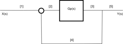
- In front of the system, before the feedback loop.
- Inside the feedback loop, in the forward path, before the plant.
- In the forward path, after the plant.
- In the feedback loop, in the reverse path.
- After the feedback loop.

Each location has certain benefits and problems, and hopefully we will get a chance to talk about all of them.
Second-Order Systems
The general expression of the transfer function of a second order system is given as:

where and are damping ratio and natural frequency of the system respectively.


Damping Ratio
The damping ratio is defined by way of the sign . The damping ratio gives us an idea about the nature of the transient response detailing the amount of overshoot & oscillation that the system will undergo. This is completely regardless of time scaling.
If :
- = zero, the system is undamped;
- < 1, the system is underdamped;
- = 1, the system is critically damped;
- > 1, the system is overdamped.
is used in conjunction with the natural frequency to determine system properties. To find the zeta value you must first find the natural response!
Natural Frequency
Natural Frequency, denoted by is defined as the frequency with which the system would oscillate if it were not damped and we define the damping ratio as .

System Sensitivity
Signal Flow Diagrams
Signal-flow graphs
Signal-flow graphs are another method for visually representing a system. Signal Flow Diagrams are especially useful, because they allow for particular methods of analysis, such as Mason's Gain Formula.
Signal flow diagrams typically use curved lines to represent wires and systems, instead of using lines at right-angles, and boxes, respectively. Every curved line is considered to have a multiplier value, which can be a constant gain value, or an entire transfer function. Signals travel from one end of a line to the other, and lines that are placed in series with one another have their total multiplier values multiplied together (just like in block diagrams).
Signal flow diagrams help us to identify structures called "loops" in a system, which can be analyzed individually to determine the complete response of the system.

Forward Paths
A forward path is a path in the signal flow diagram that connects the input to the output without touching any single node or path more than once. A single system can have multiple forward paths.
Loops
A loop is a structure in a signal flow diagram that leads back to itself. A loop does not contain the beginning and ending points, and the end of the loop is the same node as the beginning of a loop.
Loops are said to touch if they share a node or a line in common.
The Loop gain is the total gain of the loop, as you travel from one point, around the loop, back to the starting point.
Delta Values
The Delta value of a system, denoted with a Greek Δ is computed as follows:

Where:
- A is the sum of all individual loop gains
- B is the sum of the products of all the pairs of non-touching loops
- C is the sum of the products of all the sets of 3 non-touching loops
- D is the sum of the products of all the sets of 4 non-touching loops
- et cetera.
If the given system has no pairs of loops that do not touch, for instance, B and all additional letters after B will be zero.
Mason's Rule
Mason's rule is a rule for determining the gain of a system. Mason's rule can be used with block diagrams, but it is most commonly (and most easily) used with signal flow diagrams.
If we have computed our delta values (above), we can then use Mason's Gain Rule to find the complete gain of the system:
[Mason's Rule]

Where M is the total gain of the system, represented as the ratio of the output gain (yout) to the input gain (yin) of the system. Mk is the gain of the kth forward path, and Δk is the loop gain of the kth loop.
Examples
Solving a signal-flow graph by systematic reduction : Two interlocking loops
This example shows how a system of five equations in five unknowns is solved using systematic reduction rules. The independent variable is . The dependent variables are , , , , . The coefficients are labeled .


Here is the starting flowgraph:


The steps for solving follow.
Removing edge c from x2 to x3


Removing node x2 and its inflows
has no outflows, and is not a node of interest.


Removing edge e from x3 to x1


Remove edge d from x3 to x4


Node has no outflows and is not a node of interest. It is deleted along with its inflows.


Removing self-loop at x1


Removing self-loop at x4


Remove edge from x4 to x1


Remove outflow from x4 to xout

's outflow is then eliminated: is connected directly to using the product of the gains from the two edges replaced.

is not a variable of interest; thus, its node and its inflows are eliminated.

Eliminating self-loop at x1


Eliminating outflow from x1, then eliminating x1 and its inflows


is not a variable of interest; and its inflows are eliminated


Simplifying the gain expression


Solving a signal-flow graph by systematic reduction: Three equations in three unknowns
This example shows how a system of three equations in three unknowns is solved using systematic reduction rules.
The independent variables are , , . The dependent variables are , , . The coefficients are labeled . The steps for solving follow:


Electrical engineering: Construction of a flow graph for a RC circuit

This illustration shows the physical connections of the circuit. Independent voltage source S is connected in series with a resistor R and capacitor C. The example is developed from the physical circuit equations and solved using signal-flow graph techniques. Polarity is important:
- S is a source with the positive terminal at N1 and the negative terminal at N3
- R is a resistor with the positive terminal at N1 and the negative terminal at N2
- C is a capacitor with the positive terminal at N2 and the negative terminal at N3.
The unknown variable of interest is the voltage across capacitor C.
Approach to the solution:
- Find the set of equations from the physical network. These equations are acausal in nature.
- Branch equations for the capacitor and resistor. The equations will be developed as transfer functions using Laplace transforms.
- Kirchhoff's voltage and current laws
- Build a signal-flow graph from the equations.
- Solve the signal-flow graph.
Branch equations
 The branch equations are shown for R and C.
Resistor R (Branch equation )

The resistor's branch equation in the time domain is:

In the Laplace-transformed signal space:

Capacitor C (Branch equation )

The capacitor's branch equation in the time domain is:

Assuming the capacitor is initially discharged, the equation becomes:

Taking the derivative of this and multiplying by C yields the derivative form:

In the Laplace-transformed signal space:

Kirchhoff's laws equations

Kirchhoff's Voltage Law equation

This circuit has only one independent loop. Its equation in the time domain is:

In the Laplace-transformed signal space:

Kirchhoff's Current Law equations

The circuit has three nodes, thus three Kirchhoff's current equations (expresses here as the currents flowing from the nodes):

In the Laplace-transformed signal space:

A set of independent equations must be chosen. For the current laws, it is necessary to drop one of these equations. In this example, let us choose .

Building the signal-flow graph
We then look at the inventory of equations, and the signals that each equation relates:
| Equation | Signals |
|---|---|


The next step consists in assigning to each equation a signal that will be represented as a node. Each independent source signal is represented in the signal-flow graph as a source node, therefore no equation is assigned to the independent source . There are many possible valid signal flow graphs from this set of equations. An equation must only be used once, and the variables of interest must be represented.

| Equation | Signals | Assigned signal node |
|---|---|---|


The resulting flow graph is then drawn

The next step consists in solving the signal-flow graph.
Using either Mason or systematic reduction, the resulting signal flow graph is:

Mechatronics example

Bode Plots
Bode Plots
A Bode Plot is a useful tool that shows the gain and phase response of a given LTI system for different frequencies. Bode Plots are generally used with the Fourier Transform of a given system.

The frequency of the bode plots are plotted against a logarithmic frequency axis. Every tickmark on the frequency axis represents a power of 10 times the previous value. For instance, on a standard Bode plot, the values of the markers go from (0.1, 1, 10, 100, 1000, ...) Because each tickmark is a power of 10, they are referred to as a decade. Notice that the "length" of a decade decreases as you move to the right on the graph. (note that this description doesn't match the chart above... there are 10 tickmarks per decade, not one, but since it is a log chart they are not evenly spaced).
The bode Magnitude plot measures the system Input/Output ratio in special units called decibels. The Bode phase plot measures the phase shift in degrees (typically, but radians are also used).
Decibels
A Decibel is a ratio between two numbers on a logarithmic scale. To express a ratio between two numbers (A and B) as a decibel we apply the following formula for numbers that represent amplitudes (numbers that represent a power measurement use a factor of 10 rather than 20):

Where dB is the decibel result.
Or, if we just want to take the decibels of a single number C, we could just as easily write:

Frequency Response Notations
If we have a system transfer function T(s), we can separate it into a numerator polynomial N(s) and a denominator polynomial D(s). We can write this as follows:

To get the magnitude gain plot, we must first transit the transfer function into the frequency response by using the change of variables:
From here, we can say that our frequency response is a composite of two parts, a real part R and an imaginary part X:

We will use these forms below.
Straight-Line Approximations
The Bode magnitude and phase plots can be quickly and easily approximated by using a series of straight lines. These approximate graphs can be generated by following a few short, simple rules (listed below). Once the straight-line graph is determined, the actual Bode plot is a smooth curve that follows the straight lines, and travels through the breakpoints.
Break Points
If the frequency response is in pole-zero form:

We say that the values for all zn and pm are called break points of the Bode plot. These are the values where the Bode plots experience the largest change in direction.
Break points are sometimes also called "break frequencies", "cutoff points", or "corner points".
Bode Gain Plots
Bode Gain Plots, or Bode Magnitude Plots display the ratio of the system gain at each input frequency.
Bode Gain Calculations
The magnitude of the transfer function T is defined as:

However, it is frequently difficult to transition a function that is in "numerator/denominator" form to "real+imaginary" form. Luckily, our decibel calculation comes in handy. Let's say we have a frequency response defined as a fraction with numerator and denominator polynomials defined as:
If we convert both sides to decibels, the logarithms from the decibel calculations convert multiplication of the arguments into additions, and the divisions into subtractions:

And calculating out the gain of each term and adding them together will give the gain of the system at that frequency.
Bode Gain Approximations
The slope of a straight line on a Bode magnitude plot is measured in units of dB/Decade, because the units on the vertical axis are dB, and the units on the horizontal axis are decades.
The value ω = 0 is infinitely far to the left of the bode plot (because a logarithmic scale never reaches zero), so finding the value of the gain at ω = 0 essentially sets that value to be the gain for the Bode plot from all the way on the left of the graph up till the first break point. The value of the slope of the line at ω = 0 is 0 dB/Decade.
From each pole break point, the slope of the line decreases by 20 dB/Decade. The line is straight until it reaches the next break point. From each zero break point the slope of the line increases by 20 dB/Decade. Double, triple, or higher amounts of repeat poles and zeros affect the gain by multiplicative amounts. Here are some examples:
- 2 poles: -40 dB/Decade
- 10 poles: -200 dB/Decade
- 5 zeros: +100 dB/Decade
Bode Phase Plots
Bode phase plots are plots of the phase shift to an input waveform dependent on the frequency characteristics of the system input. Again, the Laplace transform does not account for the phase shift characteristics of the system, but the Fourier Transform can. The phase of a complex function, in "real+imaginary" form is given as:

Bode Procedure
Given a frequency response in pole-zero form:

Where A is a non-zero constant (can be negative or positive).
Here are the steps involved in sketching the approximate Bode magnitude plots:
Bode Magnitude Plots
- Step 1
- Factor the transfer function into pole-zero form.
- Step 2
- Find the frequency response from the Transfer function.
- Step 3
- Use logarithms to separate the frequency response into a sum of decibel terms
- Step 4
- Use to find the starting magnitude.
- Step 5
- The locations of every pole and every zero are called break points. At a zero breakpoint, the slope of the line increases by 20dB/Decade. At a pole, the slope of the line decreases by 20dB/Decade.
- Step 6
- At a zero breakpoint, the value of the actual graph differs from the value of the straight-line graph by 3dB. A zero is +3dB over the straight line, and a pole is -3dB below the straight line.
- Step 7
- Sketch the actual bode plot as a smooth-curve that follows the straight lines of the previous point, and travels through the breakpoints.

Here are the steps to drawing the Bode phase plots:
Bode Phase Plots
- Step 1
- If A is positive, start your graph (with zero slope) at 0 degrees. If A is negative, start your graph with zero slope at 180 degrees (or -180 degrees, they are the same thing).
- Step 2
- For every zero, slope the line up at 45 degrees per decade when (1 decade before the break frequency). Multiple zeros means the slope is steeper.
- Step 3
- For every pole, slope the line down at 45 degrees per decade when (1 decade before the break frequency). Multiple poles means the slope is steeper.
- Step 4
- Flatten the slope again when the phase has changed by 90 degrees (for a zero) or -90 degrees (for a pole) (or larger values, for multiple poles or multiple zeros.


Examples
Example: Constant Gain
Draw the bode plot of an amplifier system, with a constant gain increase of 6dB.
Because the gain value is constant, and is not dependent on the frequency, we know that the value of the magnitude graph is constant at all places on the graph. There are no break points, so the slope of the graph never changes. We can draw the graph as a straight, horizontal line at 6dB:

Example: Integrator
Draw the bode plot of a perfect integrator system given by the transfer function:

First, we find the frequency response of the system, by a change of variables:

Then we convert our magnitude into logarithms:

Notice that the location of the break point for the pole is located at ω → 0, which is all the way to the left of the graph. Also, we notice that inserting 0 in for ω gives us an undefined value (which approaches negative infinity, as the limit). We know, because there is a single pole at zero, that the graph to the right of zero (which is everywhere) has a slope of -20dB/Decade. We can determine from our magnitude calculation by plugging in ω → 1 that the second term drops out, and the magnitude at that point is 6dB. We now have the slope of the line, and a point that it intersects, and we can draw the graph:

Example: Differentiator


Example: 1st Order, Low-pass Filter (1 Break Point)


Further reading
Nichols Charts
Nichols Charts
This page will talk about the use of Nichols charts to analyze frequency-domain characteristics of control systems.
Stability
System stability is an important topic, because unstable systems may not perform correctly, and may actually be harmful to people. There are a number of different methods and tools that can be used to determine system stability, depending on whether you are in the state-space, or the complex domain.
Stability
Stability
When a system is unstable, the output of the system may be infinite even though the input to the system was finite. This causes a number of practical problems. For instance, a robot arm controller that is unstable may cause the robot to move dangerously. Also, systems that are unstable often incur a certain amount of physical damage, which can become costly. Nonetheless, many systems are inherently unstable - a fighter jet, for instance, or a rocket at liftoff, are examples of naturally unstable systems. Although we can design controllers that stabilize the system, it is first important to understand what stability is, how it is determined, and why it matters.
The chapters in this section are heavily mathematical and many require a background in linear differential equations. Readers without a strong mathematical background might want to review the necessary chapters in the Calculus and Ordinary Differential Equations books (or equivalent) before reading this material.
For most of this chapter we will be assuming that the system is linear and can be represented either by a set of transfer functions or in state space. Linear systems have an associated characteristic polynomial which tells us a great deal about the stability of the system. If any coefficient of the characteristic polynomial is zero or negative then the system is either unstable or at most marginally stable. It is important to note that even if all of the coefficients of the characteristic polynomial are positive the system may still be unstable. We will look into this in more detail below.
BIBO Stability
A system is defined to be BIBO Stable if every bounded input to the system results in a bounded output over the time interval . This must hold for all initial times to. So long as we don't input infinity to our system, we won't get infinity output.

A system is defined to be uniformly BIBO Stable if there exists a positive constant k that is independent of t0 such that for all t0 the following conditions:


implies that

There are a number of different types of stability, and keywords that are used with the topic of stability. Some of the important words that we are going to be discussing in this chapter, and the next few chapters are: BIBO Stable, Marginally Stable, Conditionally Stable, Uniformly Stable, Asymptotically Stable, and Unstable. All of these words mean slightly different things.
Determining BIBO Stability
We can prove mathematically that a system f is BIBO stable if an arbitrary input x is bounded by two finite but large arbitrary constants M and -M:

We apply the input x, and the arbitrary boundaries M and -M to the system to produce three outputs:


Now, all three outputs should be finite for all possible values of M and x, and they should satisfy the following relationship:

If this condition is satisfied, then the system is BIBO stable.
A SISO linear time-invariant (LTI) system is BIBO stable if and only if is absolutely integrable from [0,∞] or from:


Example
Consider the system:

We can apply our test, selecting an arbitrarily large finite constant M, and an arbitrary input x such that M>x>-M
As M approaches infinity (but does not reach infinity), we can show that:

And:

So now, we can write out our inequality:

And this inequality should be satisfied for all possible values of x. However, we can see that when x is zero, we have the following:

Which means that x is between -M and M, but the value yx is not between y-M and yM. Therefore, this system is not stable.
Poles and Stability
When the poles of the closed-loop transfer function of a given system are located in the right-half of the S-plane (RHP), the system becomes unstable. When the poles of the system are located in the left-half plane (LHP) and the system is not improper, the system is shown to be stable. A number of tests deal with this particular facet of stability: The Routh-Hurwitz Criteria, the Root-Locus, and the Nyquist Stability Criteria all test whether there are poles of the transfer function in the RHP. We will learn about all these tests in the upcoming chapters.
If the system is a multivariable, or a MIMO system, then the system is stable if and only if every pole of every transfer function in the transfer function matrix has a negative real part and every transfer function in the transfer function matrix is not improper. For these systems, it is possible to use the Routh-Hurwitz, Root Locus, and Nyquist methods described later, but these methods must be performed once for each individual transfer function in the transfer function matrix.
Poles and Eigenvalues
Every pole of G(s) is an eigenvalue of the system matrix A. However, not every eigenvalue of A is a pole of G(s).
The poles of the transfer function, and the eigenvalues of the system matrix A are related. In fact, we can say that the eigenvalues of the system matrix A are the poles of the transfer function of the system. In this way, if we have the eigenvalues of a system in the state-space domain, we can use the Routh-Hurwitz, and Root Locus methods as if we had our system represented by a transfer function instead.
On a related note, eigenvalues and all methods and mathematical techniques that use eigenvalues to determine system stability only work with time-invariant systems. In systems which are time-variant, the methods using eigenvalues to determine system stability fail.
Transfer Functions Revisited
We are going to have a brief refesher here about transfer functions, because several of the later chapters will use transfer functions for analyzing system stability.
Let us remember our generalized feedback-loop transfer function, with a gain element of K, a forward path Gp(s), and a feedback of Gb(s). We write the transfer function for this system as:

Where is the closed-loop transfer function, and is the open-loop transfer function. Again, we define the open-loop transfer function as the product of the forward path and the feedback elements, as such:


- <---Note this definition now contradicts the updated definition in the Feedback Loops section.

Now, we can define F(s) to be the characteristic equation. F(s) is simply the denominator of the closed-loop transfer function, and can be defined as such:
[Characteristic Equation]

We can say conclusively that the roots of the characteristic equation are the poles of the transfer function. Now, we know a few simple facts:
- The locations of the poles of the closed-loop transfer function determine if the system is stable or not
- The zeros of the characteristic equation are the poles of the closed-loop transfer function.
- The characteristic equation is always a simpler equation than the closed-loop transfer function.
These functions combined show us that we can focus our attention on the characteristic equation, and find the roots of that equation.
State-Space and Stability
As we have discussed earlier, the system is stable if the eigenvalues of the system matrix A have negative real parts. However, there are other stability issues that we can analyze, such as whether a system is uniformly stable, asymptotically stable, or otherwise. We will discuss all these topics in a later chapter.
Marginal Stability
When the poles of the system in the complex s-domain exist on the imaginary axis (the vertical axis), or when the eigenvalues of the system matrix are imaginary (no real part), the system exhibits oscillatory characteristics, and is said to be marginally stable. A marginally stable system may become unstable under certain circumstances, and may be perfectly stable under other circumstances. It is impossible to tell by inspection whether a marginally stable system will become unstable or not.
We will discuss marginal stability more in the following chapters.
Introduction to Digital Controls
Discrete-Time Stability
The stability analysis of a discrete-time or digital system is similar to the analysis for a continuous time system. However, there are enough differences that it warrants a separate chapter.
Input-Output Stability
Uniform Stability
An LTI causal system is uniformly BIBO stable if there exists a positive constant L such that the following conditions:
![{\displaystyle x[n_{0}]=0}](https://wikimedia.org/api/rest_v1/media/math/render/svg/b6475aebd307d5c470fd8e34059615fcb0cd4861)
![{\displaystyle \|u[n]\|\leq k}](https://wikimedia.org/api/rest_v1/media/math/render/svg/303eccf67e1d761aa092eee351727bc3108d9e09)

imply that
![{\displaystyle \|y[n]\|\leq L}](https://wikimedia.org/api/rest_v1/media/math/render/svg/9b8bf7f608ba8292dd99c8721ea388a903cfa32e)
Impulse Response Matrix
We can define the impulse response matrix of a discrete-time system as:
[Impulse Response Matrix]
![{\displaystyle G[n]=\left\{{\begin{matrix}CA^{k-1}B&{\mbox{ if }}k>0\\0&{\mbox{ if }}k\leq 0\end{matrix}}\right.}](https://wikimedia.org/api/rest_v1/media/math/render/svg/1a3c7e26c324cb2aad5a5940457bfba00e3f77ce)
Or, in the general time-varying case:
![{\displaystyle G[n]=\left\{{\begin{matrix}C\phi [n,n_{0}]B&{\mbox{ if }}k>0\\0&{\mbox{ if }}k\leq 0\end{matrix}}\right.}](https://wikimedia.org/api/rest_v1/media/math/render/svg/57c455ebe07eb605f959ad30aa1c65f4093b0783)
A digital system is BIBO stable if and only if there exists a positive constant L such that for all non-negative k:
![{\displaystyle \sum _{n=0}^{k}\|G[n]\|\leq L}](https://wikimedia.org/api/rest_v1/media/math/render/svg/4c006c870844644293fd834f0c0e1250b8fb800d)
Stability of Transfer Function
A MIMO discrete-time system is BIBO stable if and only if every pole of every transfer function in the transfer function matrix has a magnitude less than 1. All poles of all transfer functions must exist inside the unit circle on the Z plane.
Lyapunov Stability
There is a discrete version of the Lyapunov stability theorem that applies to digital systems. Given the discrete Lyapunov equation:
[Digital Lypapunov Equation]

We can use this version of the Lyapunov equation to define a condition for stability in discrete-time systems:
- Lyapunov Stability Theorem (Digital Systems)
- A digital system with the system matrix A is asymptotically stable if and only if there exists a unique matrix M that satisfies the Lyapunov Equation for every positive definite matrix N.
Poles and Eigenvalues
Every pole of G(z) is an eigenvalue of the system matrix A. Not every eigenvalue of A is a pole of G(z). Like the poles of the transfer function, all the eigenvalues of the system matrix must have magnitudes less than 1. Mathematically:

If the magnitude of the eigenvalues of the system matrix A, or the poles of the transfer functions are greater than 1, the system is unstable.
Finite Wordlengths
Digital computer systems have an inherent problem because implementable computer systems have finite wordlengths to deal with. Some of the issues are:
- Real numbers can only be represented with a finite precision. Typically, a computer system can only accurately represent a number to a finite number of decimal points.
- Because of the fact above, computer systems with feedback can compound errors with each program iteration. Small errors in one step of an algorithm can lead to large errors later in the program.
- Integer numbers in computer systems have finite lengths. Because of this, integer numbers will either roll-over, or saturate, depending on the design of the computer system. Both situations can create inaccurate results.
Routh-Hurwitz Criterion
Stability Criteria
The Routh-Hurwitz stability criterion provides a simple algorithm to decide whether or not the zeros of a polynomial are all in the left half of the complex plane (such a polynomial is called at times "Hurwitz"). A Hurwitz polynomial is a key requirement for a linear continuous-time invariant to be stable (all bounded inputs produce bounded outputs).
- Necessary stability conditions
- Conditions that must hold for a polynomial to be Hurwitz.
If any of them fails - the polynomial is not stable. However, they may all hold without implying stability.
- Sufficient stability conditions
- Conditions that if met imply that the polynomial is stable. However, a polynomial may be stable without implying some or any of them.
The Routh criteria provides condition that are both necessary and sufficient for a polynomial to be Hurwitz.
Routh-Hurwitz Criteria
The Routh-Hurwitz criteria is comprised of three separate tests that must be satisfied. If any single test fails, the system is not stable and further tests need not be performed. For this reason, the tests are arranged in order from the easiest to determine to the hardest.
The Routh Hurwitz test is performed on the denominator of the transfer function, the characteristic equation. For instance, in a closed-loop transfer function with G(s) in the forward path, and H(s) in the feedback loop, we have:

If we simplify this equation, we will have an equation with a numerator N(s), and a denominator D(s):
The Routh-Hurwitz criteria will focus on the denominator polynomial D(s).
Routh-Hurwitz Tests
Here are the three tests of the Routh-Hurwitz Criteria. For convenience, we will use N as the order of the polynomial (the value of the highest exponent of s in D(s)). The equation D(s) can be represented generally as follows:

- Rule 1
- All the coefficients ai must be present (non-zero)
- Rule 2
- All the coefficients ai must be positive (equivalently all of them must be negative, with no sign change)
- Rule 3
- If Rule 1 and Rule 2 are both satisfied, then form a Routh array from the coefficients ai. There is one pole in the right-hand s-plane for every sign change of the members in the first column of the Routh array (any sign changes, therefore, mean the system is unstable).
We will explain the Routh array below.
The Routh's Array
The Routh array is formed by taking all the coefficients ai of D(s), and staggering them in array form. The final columns for each row should contain zeros:

Therefore, if N is odd, the top row will be all the odd coefficients. If N is even, the top row will be all the even coefficients. We can fill in the remainder of the Routh Array as follows:

Now, we can define all our b, c, and other coefficients, until we reach row s0. To fill them in, we use the following formulae:

And

For each row that we are computing, we call the left-most element in the row directly above it the pivot element. For instance, in row b, the pivot element is aN-1, and in row c, the pivot element is bN-1 and so on and so forth until we reach the bottom of the array.
To obtain any element, we negate the determinant of the following matrix, and divide by the pivot element:

Where:
- k is the left-most element two rows above the current row.
- l is the pivot element.
- m is the element two rows up, and one column to the right of the current element.
- n is the element one row up, and one column to the right of the current element.
In terms of k l m n, our equation is:

Example: Calculating CN-3
To calculate the value CN-3, we must determine the values for k l m and n:
- k is the left-most element two rows up: aN-1
- l the pivot element, is the left-most element one row up: bN-1
- m is the element from one-column to the right, and up two rows: aN-5
- n is the element one column right, and one row up: bN-5
Plugging this into our equation gives us the formula for CN-3:

Example: Stable Third Order System
We are given a system with the following characteristic equation:

Using the first two requirements, we see that all the coefficients are non-zero, and all of the coefficients are positive. We will proceed then to construct the Routh-Array:

And we can calculate out all the coefficients:


And filling these values into our Routh Array, we can determine whether the system is stable:

From this array, we can clearly see that all of the signs of the first column are positive, there are no sign changes, and therefore there are no poles of the characteristic equation in the RHP.
Special Case: Row of All Zeros
If, while calculating our Routh-Hurwitz, we obtain a row of all zeros, we do not stop, but can actually learn more information about our system.
If we have a row of all zeros, the row directly above it is known as the Auxiliary Polynomial, and can be very helpful. The roots of the auxiliary polynomial give us the precise locations of complex conjugate roots that lie on the jω axis. However, one important point to notice is that if there are repeated roots on the jω axis, the system is actually unstable. Therefore, we must use the auxiliary polynomial to determine whether the roots are repeated or not.
The auxiliary equation is to be differentiated with respect to s and the coefficients of this equation replaces the all zero row. Routh array can be further calculated using these new values.
Special Case: Zero in the First Column
In this special case, there is a zero in the first column of the Routh Array, but the other elements of that row are non-zero. Like the above case, we can replace the zero with a small variable epsilon (ε) and use that variable to continue our calculations. After we have constructed the entire array, we can take the limit as epsilon approaches zero to get our final values. If the sign coefficient above the (ε) is the same as below it, this indicates a pure imaginary root.
Jury's Test
Routh-Hurwitz in Digital Systems
Because of the differences in the Z and S domains, the Routh-Hurwitz criteria can not be used directly with digital systems. This is because digital systems and continuous-time systems have different regions of stability. However, there are some methods that we can use to analyze the stability of digital systems. Our first option (and arguably not a very good option) is to convert the digital system into a continuous-time representation using the bilinear transform. The bilinear transform converts an equation in the Z domain into an equation in the W domain, that has properties similar to the S domain. Another possibility is to use Jury's Stability Test. Jury's test is a procedure similar to the RH test, except it has been modified to analyze digital systems in the Z domain directly.
Bilinear Transform
One common, but time-consuming, method of analyzing the stability of a digital system in the z-domain is to use the bilinear transform to convert the transfer function from the z-domain to the w-domain. The w-domain is similar to the s-domain in the following ways:
- Poles in the right-half plane are unstable
- Poles in the left-half plane are stable
- Poles on the imaginary axis are partially stable
The w-domain is warped with respect to the s domain, however, and except for the relative position of poles to the imaginary axis, they are not in the same places as they would be in the s-domain.
Remember, however, that the Routh-Hurwitz criterion can tell us whether a pole is unstable or not, and nothing else. Therefore, it doesn't matter where exactly the pole is, so long as it is in the correct half-plane. Since we know that stable poles are in the left-half of the w-plane and the s-plane, and that unstable poles are on the right-hand side of both planes, we can use the Routh-Hurwitz test on functions in the w domain exactly like we can use it on functions in the s-domain.
Other Mappings
There are other methods for mapping an equation in the Z domain into an equation in the S domain, or a similar domain. We will discuss these different methods in the Appendix.
Jury's Test
Jury's test is a test that is similar to the Routh-Hurwitz criterion, except that it can be used to analyze the stability of an LTI digital system in the Z domain. To use Jury's test to determine if a digital system is stable, we must check our z-domain characteristic equation against a number of specific rules and requirements. If the function fails any requirement, it is not stable. If the function passes all the requirements, it is stable. Jury's test is a necessary and sufficient test for stability in digital systems.
Again, we call D(z) the characteristic polynomial of the system. It is the denominator polynomial of the Z-domain transfer function. Jury's test will focus exclusively on the Characteristic polynomial. To perform Jury's test, we must perform a number of smaller tests on the system. If the system fails any test, it is unstable.
Jury Tests
Given a characteristic equation in the form:

The following tests determine whether this system has any poles outside the unit circle (the instability region). These tests will use the value N as being the degree of the characteristic polynomial.
The system must pass all of these tests to be considered stable. If the system fails any test, you may stop immediately: you do not need to try any further tests.
- Rule 1
- If z is 1, the system output must be positive:

- Rule 2
- If z is -1, then the following relationship must hold:

- Rule 3
- The absolute value of the constant term (a0) must be less than the value of the highest coefficient (aN):

If Rule 1 Rule 2 and Rule 3 are satisified, construct the Jury Array (discussed below).
- Rule 4
- Once the Jury Array has been formed, all the following relationships must be satisifed until the end of the array:
- And so on until the last row of the array. If all these conditions are satisifed, the system is stable.


While you are constructing the Jury Array, you can be making the tests of Rule 4. If the Array fails Rule 4 at any point, you can stop calculating the array: your system is unstable. We will discuss the construction of the Jury Array below.
The Jury Array
The Jury Array is constructed by first writing out a row of coefficients, and then writing out another row with the same coefficients in reverse order. For instance, if your polynomial is a third order system, we can write the First two lines of the Jury Array as follows:

Now, once we have the first row of our coefficients written out, we add another row of coefficients (we will use b for this row, and c for the next row, as per our previous convention), and we will calculate the values of the lower rows from the values of the upper rows. Each new row that we add will have one fewer coefficient then the row before it:

Note: The last file is the (2N-3) file, and always has 3 elements. This test doesn't have sense if N=1, but in this case you know the pole!
Once we get to a row with 2 members, we can stop constructing the array.
To calculate the values of the odd-number rows, we can use the following formulae. The even number rows are equal to the previous row in reverse order. We will use k as an arbitrary subscript value. These formulae are reusable for all elements in the array:


This pattern can be carried on to all lower rows of the array, if needed.
Example: Calculating e5
Give the equation for member e5 of the jury array (assuming the original polynomial is sufficiently large to require an e5 member).
Going off the pattern we set above, we can have this equation for a member e:

Where we are using R as the subtractive element from the above equations. Since row c had R → 1, and row d had R → 2, we can follow the pattern and for row e set R → 3. Plugging this value of R into our equation above gives us:

And since we want e5 we know that k is 5, so we can substitute that into the equation:

When we take the determinant, we get the following equation:

Further reading
We will discuss the bilinear transform, and other methods to convert between the Laplace domain and the Z domain in the appendix:
Root Locus
The Problem
Consider a system like a radio. The radio has a "volume" knob, that controls the amount of gain of the system. High volume means more power going to the speakers, low volume means less power to the speakers. As the volume value increases, the poles of the transfer function of the radio change, and they might potentially become unstable. We would like to find out if the radio becomes unstable, and if so, we would like to find out what values of the volume cause it to become unstable. Our current methods would require us to plug in each new value for the volume (gain, "K"), and solve the open-loop transfer function for the roots. This process can be a long one. Luckily, there is a method called the root-locus method, that allows us to graph the locations of all the poles of the system for all values of gain, K
Root-Locus
As we change gain, we notice that the system poles and zeros actually move around in the S-plane. This fact can make life particularly difficult, when we need to solve higher-order equations repeatedly, for each new gain value. The solution to this problem is a technique known as Root-Locus graphs. Root-Locus allows you to graph the locations of the poles and zeros for every value of gain, by following several simple rules. As we know that a fan switch also can control the speed of the fan.
Let's say we have a closed-loop transfer function for a particular system:

Where N is the numerator polynomial and D is the denominator polynomial of the transfer functions, respectively. Now, we know that to find the poles of the equation, we must set the denominator to 0, and solve the characteristic equation. In other words, the locations of the poles of a specific equation must satisfy the following relationship:

from this same equation, we can manipulate the equation as such:


And finally by converting to polar coordinates:

Now we have 2 equations that govern the locations of the poles of a system for all gain values:
[The Magnitude Equation]
[The Angle Equation]
Digital Systems
The same basic method can be used for considering digital systems in the Z-domain:

Where N is the numerator polynomial in z, D is the denominator polynomial in z, and is the open-loop transfer function of the system, in the Z domain.

The denominator D(z), by the definition of the characteristic equation is equal to:

We can manipulate this as follows:


We can now convert this to polar coordinates, and take the angle of the polynomial:

We are now left with two important equations:
[The Magnitude Equation]
[The Angle Equation]
If you will compare the two, the Z-domain equations are nearly identical to the S-domain equations, and act exactly the same. For the remainder of the chapter, we will only consider the S-domain equations, with the understanding that digital systems operate in nearly the same manner.
The Root-Locus Procedure
In this section, the rules for the S-Plane and the Z-plane are the same, so we won't refer to the differences between them.
In the transform domain (see note at right), when the gain is small, the poles start at the poles of the open-loop transfer function. When gain becomes infinity, the poles move to overlap the zeros of the system. This means that on a root-locus graph, all the poles move towards a zero. Only one pole may move towards one zero, and this means that there must be the same number of poles as zeros.
If there are fewer zeros than poles in the transfer function, there are a number of implicit zeros located at infinity, that the poles will approach.
First thing, we need to convert the magnitude equation into a slightly more convenient form:

We generally use capital letters for functions in the frequency domain, but a(s) and b(s) are unimportant enough to be lower-case.
Now, we can assume that G(s)H(s) is a fraction of some sort, with a numerator and a denominator that are both polynomials. We can express this equation using arbitrary functions a(s) and b(s), as such:

We will refer to these functions a(s) and b(s) later in the procedure.
We can start drawing the root-locus by first placing the roots of b(s) on the graph with an 'X'. Next, we place the roots of a(s) on the graph, and mark them with an 'O'.
Poles are marked on the graph with an 'X' and zeros are marked with an 'O' by common convention. These letters have no particular meaning |
Next, we examine the real-axis. starting from the right-hand side of the graph and traveling to the left, we draw a root-locus line on the real-axis at every point to the left of an odd number of poles or zeros on the real-axis. This may sound tricky at first, but it becomes easier with practice.
Double poles or double zeros count as two. |
Now, a root-locus line starts at every pole. Therefore, any place that two poles appear to be connected by a root locus line on the real-axis, the two poles actually move towards each other, and then they "break away", and move off the axis. The point where the poles break off the axis is called the breakaway point. From here, the root locus lines travel towards the nearest zero.
It is important to note that the s-plane is symmetrical about the real axis, so whatever is drawn on the top-half of the S-plane, must be drawn in mirror-image on the bottom-half plane.
Once a pole breaks away from the real axis, they can either travel out towards infinity (to meet an implicit zero), or they can travel to meet an explicit zero, or they can re-join the real-axis to meet a zero that is located on the real-axis. If a pole is traveling towards infinity, it always follows an asymptote. The number of asymptotes is equal to the number of implicit zeros at infinity.
Root Locus Rules
Here is the complete set of rules for drawing the root-locus graph. We will use p and z to denote the number of poles and the number of zeros of the open-loop transfer function, respectively. We will use Pi and Zi to denote the location of the ith pole and the ith zero, respectively. Likewise, we will use ψi and ρi to denote the angle from a given point to the ith pole and zero, respectively. All angles are given in radians (π denotes π radians).
There are 11 rules that, if followed correctly, will allow you to create a correct root-locus graph.
- Rule 1
- There is one branch of the root-locus for every root of b(s).
- Rule 2
- The roots of b(s) are the poles of the open-loop transfer function. Mark the roots of b(s) on the graph with an X.
- Rule 3
- The roots of a(s) are the zeros of the open-loop transfer function. Mark the roots of a(s) on the graph with an O. There should be a number of O's less than or equal to the number of X's. There is a number of zeros p - z located at infinity. These zeros at infinity are called "implicit zeros". All branches of the root-locus will move from a pole to a zero (some branches, therefore, may travel towards infinity).
- Rule 4
- A point on the real axis is a part of the root-locus if it is to the left of an odd number of poles and zeros.
- Rule 5
- The gain at any point on the root locus can be determined by the inverse of the absolute value of the magnitude equation.

- Rule 6
- The root-locus diagram is symmetric about the real-axis. All complex roots are conjugates.
- Rule 7
- Two roots that meet on the real-axis will break away from the axis at certain break-away points. If we set s → σ (no imaginary part), we can use the following equation:
- And differentiate to find the local maximum:


- Rule 8
- The breakaway lines of the root locus are separated by angles of , where α is the number of poles intersecting at the breakaway point.
- Rule 9
- The breakaway root-loci follow asymptotes that intersect the real axis at angles φω given by:
- The origin of these asymptotes, OA, is given as the sum of the pole locations, minus the sum of the zero locations, divided by the difference between the number of poles and zeros:
- The OA point should lie on the real axis.
- Rule 10
- The branches of the root locus cross the imaginary axis at points where the angle equation value is π (i.e., 180o).
- Rule 11
- The angles that the root locus branch makes with a complex-conjugate pole or zero is determined by analyzing the angle equation at a point infinitessimally close to the pole or zero. The angle of departure, φd is given by the following equation:
- The angle of arrival, φa, is given by:


We will explain these rules in the rest of the chapter.
Root Locus Equations
Here are the two major equations:
[Root Locus Equations]
S-Domain Equations Z-Domain Equations


Note that the sum of the angles of all the poles and zeros must equal to 180.
Number of Asymptotes
If the number of explicit zeros of the system is denoted by Z (uppercase z), and the number of poles of the system is given by P, then the number of asymptotes (Na) is given by:
[Number of Asymptotes]

The angles of the asymptotes are given by:
[Angle of Asymptotes]

for values of .
![{\displaystyle k=[0,1,...N_{a}-1]}](https://wikimedia.org/api/rest_v1/media/math/render/svg/94ac7e6cea982087fc9d43f05ef29150b814bbb5)
The angles for the asymptotes are measured from the positive real-axis |
Asymptote Intersection Point
The asymptotes intersect the real axis at the point:
[Origin of Asymptotes]

Where is the sum of all the locations of the poles, and is the sum of all the locations of the explicit zeros.


Breakaway Points
The breakaway points are located at the roots of the following equation:
[Breakaway Point Locations]
- or


Once you solve for z, the real roots give you the breakaway/reentry points. Complex roots correspond to a lack of breakaway/reentry.
The breakaway point equation can be difficult to solve, so many times the actual location is approximated.
Root Locus and Stability
The root locus procedure should produce a graph of where the poles of the system are for all values of gain K. When any or all of the roots of D are in the unstable region, the system is unstable. When any of the roots are in the marginally stable region, the system is marginally stable (oscillatory). When all of the roots of D are in the stable region, then the system is stable.
It is important to note that a system that is stable for gain K1 may become unstable for a different gain K2. Some systems may have poles that cross over from stable to unstable multiple times, giving multiple gain values for which the system is unstable.
Here is a quick refresher:
Region S-Domain Z-Domain Stable Region Left-Hand S Plane Inside the Unit Circle Marginally Stable Region The vertical axis The Unit Circle Unstable Region Right-Hand S Plane Outside the Unit Circle,


Examples
Example 1: First-Order System
Find the root-locus of the open-loop system:

If we look at the characteristic equation, we can quickly solve for the single pole of the system:


We plot that point on our root-locus graph, and everything on the real axis to the left of that single point is on the root locus (from the rules, above). Therefore, the root locus of our system looks like this:

From this image, we can see that for all values of gain this system is stable.
Example 2: Third Order System
We are given a system with three real poles, shown by the transfer function:

Is this system stable?
To answer this question, we can plot the root-locus. First, we draw the poles on the graph at locations -1, -2, and -3. The real-axis between the first and second poles is on the root-locus, as well as the real axis to the left of the third pole. We know also that there is going to be breakaway from the real axis at some point. The origin of asymptotes is located at:
- ,

and the angle of the asymptotes is given by:

We know that the breakaway occurs between the first and second poles, so we will estimate the exact breakaway point. Drawing the root-locus gives us the graph below.

We can see that for low values of gain the system is stable, but for higher values of gain, the system becomes unstable.
Example: Complex-Conjugate Zeros
Find the root-locus graph for the following system transfer function:

If we look at the denominator, we have poles at the origin, -1, and -2. Following Rule 4, we know that the real-axis between the first two poles, and the real axis after the third pole are all on the root-locus. We also know that there is going to be a breakaway point between the first two poles, so that they can approach the complex conjugate zeros. If we use the quadratic equation on the numerator, we can find that the zeros are located at:

If we draw our graph, we get the following:
We can see from this graph that the system is stable for all values of K.
Example: Root-Locus Using MATLAB/Octave
{{TextBox|1=Use MATLAB, Octave, or another piece of mathematical simulation software to produce the root-locus graph for the following system:

First, we must multiply through in the denominator:


Now, we can generate the coefficient vectors from the numerator and denominator:
 num = [0 1 7 12];
 den = [0 1 3 2];
Next, we can feed these vectors into the rlocus command:
rlocus(num, den);
Note:In Octave, we need to create a system structure first, by typing:
 sys = tf(num, den);
 rlocus(sys);
Either way, we generate the following graph:

Nyquist Criterion
Nyquist Stability Criteria
The Nyquist Stability Criteria is a test for system stability, just like the Routh-Hurwitz test, or the Root-Locus Methodology. However, the Nyquist Criteria can also give us additional information about a system. Routh-Hurwitz and Root-Locus can tell us where the poles of the system are for particular values of gain. By altering the gain of the system, we can determine if any of the poles move into the RHP, and therefore become unstable. The Nyquist Criteria, however, can tell us things about the frequency characteristics of the system. For instance, some systems with constant gain might be stable for low-frequency inputs, but become unstable for high-frequency inputs.
Here is an example of a system responding differently to different frequency input values: Consider an ordinary glass of water. If the water is exposed to ordinary sunlight, it is unlikely to heat up too much. However, if the water is exposed to microwave radiation (from inside your microwave oven, for instance), the water will quickly heat up to a boil.
Also, the Nyquist Criteria can tell us things about the phase of the input signals, the time-shift of the system, and other important information.
Contours
A contour is a complicated mathematical construct, but luckily we only need to worry ourselves with a few points about them. We will denote contours with the Greek letter Γ (gamma). Contours are lines, drawn on a graph, that follow certain rules:
- The contour must close (it must form a complete loop)
- The contour may not cross directly through a pole of the system.
- Contours must have a direction (clockwise or counterclockwise, generally).
- A contour is called "simple" if it has no self-intersections. We only consider simple contours here.
Once we have such a contour, we can develop some important theorems about them, and finally use these theorems to derive the Nyquist stability criterion.
Argument Principle
Here is the argument principle, which we will use to derive the stability criterion. Do not worry if you do not understand all the terminology, we will walk through it:
- The Argument Principle
- If we have a contour, Γ, drawn in one plane (say the complex laplace plane, for instance), we can map that contour into another plane, the F(s) plane, by transforming the contour with the function F(s). The resultant contour, will circle the origin point of the F(s) plane N times, where N is equal to the difference between Z and P (the number of zeros and poles of the function F(s), respectively).

When we have our contour, Γ, we transform it into by plugging every point of the contour into the function F(s), and taking the resultant value to be a point on the transformed contour.
Example: First Order System
Let's say, for instance, that Γ is a unit square contour in the complex s plane. The vertices of the square are located at points I,J,K,L, as follows:


we must also specify the direction of our contour, and we will say (arbitrarily) that it is a clockwise contour (travels from I to J to K to L). We will also define our transform function, F(s), to be the following:

We can factor the denominator of F(s), and we can show that there is one zero at s → -0.5, and no poles. Plotting this root on the same graph as our contour, we see clearly that it lies within the contour. Since s is a complex variable, defined with real and imaginary parts as:
We know that F(s) must also be complex. We will say, for reasons of simplicity, that the axes in the F(s) plane are u and v, and are related as such:

From this relationship, we can define u and v in terms of σ and ω:


Now, to transform Γ, we will plug every point of the contour into F(s), and the resultant values will be the points of . We will solve for complex values u and v, and we will start with the vertices, because they are the simplest examples:


We can take the lines in between the vertices as a function of s, and plug the entire function into the transform. Luckily, because we are using straight lines, we can simplify very much:
- Line from I to J:
- Line from J to K:
- Line from K to L:
- Line from L to I:


And when we graph these functions, from vertex to vertex, we see that the resultant contour in the F(s) plane is a square, but not centered at the origin, and larger in size. Notice how the contour encircles the origin of the F(s) plane one time. This will be important later on.
Example: Second-Order System
Let's say that we have a slightly more complicated mapping function:

We can see clearly that F(s) has a zero at s → -0.5, and a complex conjugate set of poles at s → -0.5 + 0.5j and s → -0.5 - 0.5j. We will use the same unit square contour, Γ, from above:
We can see clearly that the poles and the zero of F(s) lie within Γ. Setting F(s) to u + vj and solving, we get the following relationships:

This is a little difficult now, because we need to simplify this whole expression, and separate it out into real and imaginary parts. There are two methods to doing this, neither of which is short or easy enough to demonstrate here to entirety:
- We convert the numerator and denominator polynomials into a polar representation in terms of r and θ, then perform the division, and then convert back into rectangular format.
- We plug each segment of our contour into this equation, and simplify numerically.
The Nyquist Contour
The Nyquist contour, the contour that makes the entire nyquist criterion work, must encircle the entire unstable region of the complex plane. For analog systems, this is the right half of the complex s plane. For digital systems, this is the entire plane outside the unit circle. Remember that if a pole to the closed-loop transfer function (or equivalently a zero of the characteristic equation) lies in the unstable region of the complex plane, the system is an unstable system.
- Analog Systems
- The Nyquist contour for analog systems is an infinite semi-circle that encircles the entire right-half of the s plane. The semicircle travels up the imaginary axis from negative infinity to positive infinity. From positive infinity, the contour breaks away from the imaginary axis, in the clock-wise direction, and forms a giant semicircle.
- Digital Systems
- The Nyquist contour in digital systems is a counter-clockwise encirclement of the unit circle.
Nyquist Criteria
Let us first introduce the most important equation when dealing with the Nyquist criterion:

Where:
- N is the number of encirclements of the (-1, 0) point.
- Z is the number of zeros of the characteristic equation.
- P is the number of poles in the of the open-loop characteristic equation.
With this equation stated, we can now state the Nyquist Stability Criterion:
- Nyquist Stability Criterion
- A feedback control system is stable, if and only if the contour in the F(s) plane does not encircle the (-1, 0) point when P is 0.
- A feedback control system is stable, if and only if the contour in the F(s) plane encircles the (-1, 0) point a number of times equal to the number of poles of F(s) enclosed by Γ.
In other words, if P is zero then N must equal zero. Otherwise, N must equal P. Essentially, we are saying that Z must always equal zero, because Z is the number of zeros of the characteristic equation (and therefore the number of poles of the closed-loop transfer function) that are in the right-half of the s plane.
Keep in mind that we don't necessarily know the locations of all the zeros of the characteristic equation. So if we find, using the nyquist criterion, that the number of poles is not equal to N, then we know that there must be a zero in the right-half plane, and that therefore the system is unstable.
Nyquist ↔ Bode
A careful inspection of the Nyquist plot will reveal a surprising relationship to the Bode plots of the system. If we use the Bode phase plot as the angle θ, and the Bode magnitude plot as the distance r, then it becomes apparent that the Nyquist plot of a system is simply the polar representation of the Bode plots.
To obtain the Nyquist plot from the Bode plots, we take the phase angle and the magnitude value at each frequency ω. We convert the magnitude value from decibels back into gain ratios. Then, we plot the ordered pairs (r, θ) on a polar graph.
Nyquist in the Z Domain
The Nyquist Criteria can be utilized in the digital domain in a similar manner as it is used with analog systems. The primary difference in using the criteria is that the shape of the Nyquist contour must change to encompass the unstable region of the Z plane. Therefore, instead of an infinitesimal semi-circle, the Nyquist contour for digital systems is a counter-clockwise unit circle. By changing the shape of the contour, the same N = Z - P equation holds true, and the resulting Nyquist graph will typically look identical to one from an analog system, and can be interpreted in the same way.
State-Space Stability
State-Space Stability
If a system is represented in the state-space domain, it doesn't make sense to convert that system to a transfer function representation (or even a transfer matrix representation) in an attempt to use any of the previous stability methods. Luckily, there are other analysis methods that can be used with the state-space representation to determine if a system is stable or not. First, let us first introduce the notion of unstability:
- Unstable
- A system is said to be unstable if the system response approaches infinity as time approaches infinity. If our system is G(t), then, we can say a system is unstable if:

Also, a key concept when we are talking about stability of systems is the concept of an equilibrium point:
- Equilibrium Point
- Given a system f such that:

A particular state xe is called an equilibrium point if

for all time t in the interval , where t0 is the starting time of the system.
The definitions below typically require that the equilibrium point be zero. If we have an equilibrium point xe = a, then we can use the following change of variables to make the equilibrium point zero:

We will also see below that a system's stability is defined in terms of an equilibrium point. Related to the concept of an equilibrium point is the notion of a zero point:
- Zero State
- A state xz is a zero state if xz = 0. A zero state may or may not be an equilibrium point.
Stability Definitions
The equilibrium x = 0 of the system is stable if and only if the solutions of the zero-input state equation are bounded. Equivalently, x = 0 is a stable equilibrium if and only if for every initial time t0, there exists an associated finite constant k(t0) such that:

Where sup is the supremum, or "maximum" value of the equation. The maximum value of this equation must never exceed the arbitrary finite constant k (and therefore it may not be infinite at any point).
- Uniform Stability
- The system is defined to be uniformly stable if it is stable for all initial values of t0:
![{\displaystyle \operatorname {sup} _{t\geq 0}[\operatorname {sup} _{t\geq t_{0}}\|\phi (t,t_{0})\|]=k_{0}<\infty }](https://wikimedia.org/api/rest_v1/media/math/render/svg/b693a4c15c1084ec796619154d0d88321e8a2154)
Uniform stability is a more general, and more powerful form of stability than was previously provided.
- Asymptotic Stability
- A system is defined to be asymptotically stable if:

A time-invariant system is asymptotically stable if all the eigenvalues of the system matrix A have negative real parts. If a system is asymptotically stable, it is also BIBO stable. However the inverse is not true: A system that is BIBO stable might not be asymptotically stable.
- Uniform Asymptotic Stability
- A system is defined to be uniformly asymptotically stable if the system is asymptotically stable for all values of t0.
- Exponential Stability
- A system is defined to be exponentially stable if the system response decays exponentially towards zero as time approaches infinity.
For linear systems, uniform asymptotic stability is the same as exponential stability. This is not the case with non-linear systems.
Marginal Stability
Here we will discuss some rules concerning systems that are marginally stable. Because we are discussing eigenvalues and eigenvectors, these theorems only apply to time-invariant systems.
- A time-invariant system is marginally stable if and only if all the eigenvalues of the system matrix A are zero or have negative real parts, and those with zero real parts are simple roots of the minimal polynomial of A.
- The equilibrium x = 0 of the state equation is uniformly stable if all eigenvalues of A have non-positive real parts, and there is a complete set of distinct eigenvectors associated with the eigenvalues with zero real parts.
- The equilibrium x = 0 of the state equation is exponentially stable if and only if all eigenvalues of the system matrix A have negative real parts.
Eigenvalues and Poles
A Linearly Time Invariant (LTI) system is stable (asymptotically stable, see above) if all the eigenvalues of A have negative real parts. Consider the following state equation:
We can take the Laplace Transform of both sides of this equation, using initial conditions of x0 = 0:

Subtract AX(s) from both sides:


Assuming (sI - A) is nonsingular, we can multiply both sides by the inverse:

Now, if we remember our formula for finding the matrix inverse from the adjoint matrix:

We can use that definition here:

Let's look at the denominator (which we will now call D(s)) more closely. To be stable, the following condition must be true:

And if we substitute λ for s, we see that this is actually the characteristic equation of matrix A! This means that the values for s that satisfy the equation (the poles of our transfer function) are precisely the eigenvalues of matrix A. In the S domain, it is required that all the poles of the system be located in the left-half plane, and therefore all the eigenvalues of A must have negative real parts.
Impulse Response Matrix
We can define the Impulse response matrix, G(t, τ) in order to define further tests for stability:
[Impulse Response Matrix]

The system is uniformly stable if and only if there exists a finite positive constant L such that for all time t and all initial conditions t0 with the following integral is satisfied:

In other words, the above integral must have a finite value, or the system is not uniformly stable.
In the time-invariant case, the impulse response matrix reduces to:

In a time-invariant system, we can use the impulse response matrix to determine if the system is uniformly BIBO stable by taking a similar integral:

Where L is a finite constant.
Positive Definiteness
These terms are important, and will be used in further discussions on this topic.
- f(x) is positive definite if f(x) > 0 for all x.
- f(x) is positive semi-definite if for all x, and f(x) = 0 only if x = 0.
- f(x) is negative definite if f(x) < 0 for all x.
- f(x) is negative semi-definite if for all x, and f(x) = 0 only if x = 0.


A Hermitian matrix X is positive definite if all its principle minors are positive. Also, a matrix X is positive definite if all its eigenvalues have positive real parts. These two methods may be used interchangeably.
Positive definiteness is a very important concept. So much so that the Lyapunov stability test depends on it. The other categorizations are not as important, but are included here for completeness.
Lyapunov Stability
Lyapunov's Equation
For linear systems, we can use the Lyapunov Equation, below, to determine if a system is stable. We will state the Lyapunov Equation first, and then state the Lyapunov Stability Theorem.
[Lyapunov Equation]

Where A is the system matrix, and M and N are p × p square matrices.
- Lyapunov Stability Theorem
- An LTI system is stable if there exists a matrix M that satisfies the Lyapunov Equation where N is an arbitrary positive definite matrix, and M is a unique positive definite matrix.

Notice that for the Lyapunov Equation to be satisfied, the matrices must be compatible sizes. In fact, matrices A, M, and N must all be square matrices of equal size. Alternatively, we can write:
- Lyapunov Stability Theorem (alternate)
- If all the eigenvalues of the system matrix A have negative real parts, then the Lyapunov Equation has a unique solution M for every positive definite matrix N, and the solution can be calculated by:

If the matrix M can be calculated in this manner, the system is asymptotically stable.
Controllers and Compensators
There are a number of preexisting devices for use in system control, such as lead and lag compensators, and powerful PID controllers. PID controllers are so powerful that many control engineers may use no other method of system control! The chapters in this section will discuss some of the common types of system compensators and controllers.
Controllability and Observability
System Interaction
In the world of control engineering, there are a slew of systems available that need to be controlled. The task of a control engineer is to design controller and compensator units to interact with these pre-existing systems. However, some systems simply cannot be controlled (or, more often, cannot be controlled in specific ways). The concept of controllability refers to the ability of a controller to arbitrarily alter the functionality of the system plant.
The state-variable of a system, x, represents the internal workings of the system that can be separate from the regular input-output relationship of the system. This also needs to be measured, or observed. The term observability describes whether the internal state variables of the system can be externally measured.
Controllability
Complete state controllability (or simply controllability if no other context is given) describes the ability of an external input to move the internal state of a system from any initial state to any other final state in a finite time interval
We will start off with the definitions of the term controllability, and the related terms reachability and stabilizability.
- Controllability
- A system with internal state vector x is called controllable if and only if the system states can be changed by changing the system input.
- Reachability
- A particular state x1 is called reachable if there exists an input that transfers the state of the system from the initial state x0 to x1 in some finite time interval [t0, t).
- Stabilizability
- A system is Stabilizable if all states that cannot be reached decay to zero asymptotically.
We can also write out the definition of reachability more precisely:
A state x1 is called reachable at time t1 if for some finite initial time t0 there exists an input u(t) that transfers the state x(t) from the origin at t0 to x1.
A system is reachable at time t1 if every state x1 in the state-space is reachable at time t1.
Similarly, we can more precisely define the concept of controllability:
A state x0 is controllable at time t0 if for some finite time t1 there exists an input u(t) that transfers the state x(t) from x0 to the origin at time t1.
A system is called controllable at time t0 if every state x0 in the state-space is controllable.
Controllability Matrix
For LTI (linear time-invariant) systems, a system is reachable if and only if its controllability matrix, ζ, has a full row rank of p, where p is the dimension of the matrix A, and p × q is the dimension of matrix B.
[Controllability Matrix]

A system is controllable or "Controllable to the origin" when any state x1 can be driven to the zero state x = 0 in a finite number of steps.
A system is controllable when the rank of the system matrix A is p, and the rank of the controllability matrix is equal to:

If the second equation is not satisfied, the system is not .
MATLAB allows one to easily create the controllability matrix with the ctrb command. To create the controllability matrix simply type

where A and B are mentioned above. Then in order to determine if the system is controllable or not one can use the rank command to determine if it has full rank.
If

Then controllability does not imply reachability.
- Reachability always implies controllability.
- Controllability only implies reachability when the state transition matrix is nonsingular.
Determining Reachability
There are four methods that can be used to determine if a system is reachable or not:
- If the p rows of are linearly independent over the field of complex numbers. That is, if the rank of the product of those two matrices is equal to p for all values of t and τ
- If the rank of the controllability matrix is the same as the rank of the system matrix A.
- If the rank of for all eigenvalues λ of the matrix A.
- If the rank of the reachability gramian (described below) is equal to the rank of the system matrix A.

![{\displaystyle \operatorname {rank} [\lambda I-A,B]=p}](https://wikimedia.org/api/rest_v1/media/math/render/svg/0b340340b41e8c39dfe637e3766968cb57648af0)
Each one of these conditions is both necessary and sufficient. If any one test fails, all the tests will fail, and the system is not reachable. If any test is positive, then all the tests will be positive, and the system is reachable.
Gramians
Gramians are complicated mathematical functions that can be used to determine specific things about a system. For instance, we can use gramians to determine whether a system is controllable or reachable. Gramians, because they are more complicated than other methods, are typically only used when other methods of analyzing a system fail (or are too difficult).
All the gramians presented on this page are all matrices with dimension p × p (the same size as the system matrix A).
All the gramians presented here will be described using the general case of Linear time-variant systems. To change these into LTI (time-invariant equations), the following substitutions can be used:


Where we are using the notation X' to denote the transpose of a matrix X (as opposed to the traditional notation XT).
Reachability Gramian
We can define the reachability gramian as the following integral:
[Reachability Gramian]

The system is reachable if the rank of the reachability gramian is the same as the rank of the system matrix:

<chemistry>/control{range}
Controllability Gramian
We can define the controllability gramian of a system (A, B) as:
[Controllability Gramian]

The system is controllable if the rank of the controllability gramian is the same as the rank of the system matrix:

If the system is time-invariant, there are two important points to be made. First, the reachability gramian and the controllability gramian reduce to be the same equation. Therefore, for LTI systems, if we have found one gramian, then we automatically know both gramians. Second, the controllability gramian can also be found as the solution to the following Lyapunov equation:

Many software packages, notably MATLAB, have functions to solve the Lyapunov equation. By using this last relation, we can also solve for the controllability gramian using these existing functions.
Observability
The state-variables of a system might not be able to be measured for any of the following reasons:
- The location of the particular state variable might not be physically accessible (a capacitor or a spring, for instance).
- There are no appropriate instruments to measure the state variable, or the state-variable might be measured in units for which there does not exist any measurement device.
- The state-variable is a derived "dummy" variable that has no physical meaning.
If things cannot be directly observed, for any of the reasons above, it can be necessary to calculate or estimate the values of the internal state variables, using only the input/output relation of the system, and the output history of the system from the starting time. In other words, we must ask whether or not it is possible to determine what the inside of the system (the internal system states) is like, by only observing the outside performance of the system (input and output)? We can provide the following formal definition of mathematical observability:
- Observability
- A system with an initial state, is observable if and only if the value of the initial state can be determined from the system output y(t) that has been observed through the time interval . If the initial state cannot be so determined, the system is unobservable.


- Complete Observability
- A system is said to be completely observable if all the possible initial states of the system can be observed. Systems that fail this criteria are said to be unobservable.
- Detectability
- A system is Detectable if all states that cannot be observed decay to zero asymptotically.
- Constructability
- A system is constructable if the present state of the system can be determined from the present and past outputs and inputs to the system. If a system is observable, then it is also constructable. The relationship does not work the other way around.
A system state xi is unobservable at a given time ti if the zero-input response of the system is zero for all time t. If a system is observable, then the only state that produces a zero output for all time is the zero state. We can use this concept to define the term state-observability.
- State-Observability
- A system is completely state-observable at time t0 or the pair (A, C) is observable at t0 if the only state that is unobservable at t0 is the zero state x = 0.
Constructability
A state x is unconstructable at a time t1 if for every finite time t < t1 the zero input response of the system is zero for all time t.
A system is completely state constructable at time t1 if the only state x that is unconstructable at t0 is x = 0.
If a system is observable at an initial time t0, then it is constructable at some time t > t0, if it is constructable at t1.
Observability Matrix
The observability of the system is dependent only on the system states and the system output, so we can simplify our state equations to remove the input terms:
Matrix Dimensions:
A: p × p
B: p × q
C: r × p
D: r × q


Therefore, we can show that the observability of the system is dependent only on the coefficient matrices A and C. We can show precisely how to determine whether a system is observable, using only these two matrices. If we have the observability matrix Q:
[Observability Matrix]

we can show that the system is observable if and only if the Q matrix has a rank of p. Notice that the Q matrix has the dimensions pr × p.
MATLAB allows one to easily create the observability matrix with the obsv command. To create the observability matrix simply type

- Q=obsv(A,C)
where A and C are mentioned above. Then in order to determine if the system is observable or not one can use the rank command to determine if it has full rank.
Observability Gramian
We can define an observability gramian as:
[Observability Gramian]

A system is completely state observable at time t0 < t < t1 if and only if the rank of the observability gramian is equal to the size p of the system matrix A.
If the system (A, B, C, D) is time-invariant, we can construct the observability gramian as the solution to the Lyapunov equation:

Constructability Gramian
We can define a constructability gramian as:
[Constructability Gramian]

A system is completely state observable at an initial time t0 if and only if there exists a finite t1 such that:

Notice that the constructability and observability gramians are very similar, and typically they can both be calculated at the same time, only substituting in different values into the state-transition matrix.
Duality Principle
The concepts of controllability and observability are very similar. In fact, there is a concrete relationship between the two. We can say that a system (A, B) is controllable if and only if the system (A', C, B', D) is observable. This fact can be proven by plugging A' in for A, and B' in for C into the observability Gramian. The resulting equation will exactly mirror the formula for the controllability gramian, implying that the two results are the same.
System Specifications
System Specification
There are a number of different specifications that might need to be met by a new system design. In this chapter we will talk about some of the specifications that systems use, and some of the ways that engineers analyze and quantify technical systems.
Steady-State Accuracy
Sensitivity
The sensitivity of a system is a parameter that is specified in terms of a given output and a given input. The sensitivity measures how much change is caused in the output by small changes to the reference input. Sensitive systems have very large changes in output in response to small changes in the input. The sensitivity of system H to input X is denoted as:

Disturbance Rejection
All physically-realized systems have to deal with a certain amount of noise and disturbance. The ability of a system to reject the noise is known as the disturbance rejection of the system.
Control Effort
The control effort is the amount of energy or power necessary for the controller to perform its duty.
Controllers and Compensators
Controllers
There are a number of different standard types of control systems that have been studied extensively. These controllers, specifically the P, PD, PI, and PID controllers are very common in the production of physical systems, but as we will see they each carry several drawbacks.
Proportional Controllers

Proportional controllers are simply gain values. These are essentially multiplicative coefficients, usually denoted with a K. A P controller can only force the system poles to a spot on the system's root locus. A P controller cannot be used for arbitrary pole placement.
We refer to this kind of controller by a number of different names: proportional controller, gain, and zeroth-order controller.
Derivative Controllers

In the Laplace domain, we can show the derivative of a signal using the following notation:

Since most systems that we are considering have zero initial condition, this simplifies to:

The derivative controllers are implemented to account for future values, by taking the derivative, and controlling based on where the signal is going to be in the future. Derivative controllers should be used with care, because even small amount of high-frequency noise can cause very large derivatives, which appear like amplified noise. Also, derivative controllers are difficult to implement perfectly in hardware or software, so frequently solutions involving only integral controllers or proportional controllers are preferred over using derivative controllers.
Notice that derivative controllers are not proper systems, in that the order of the numerator of the system is greater than the order of the denominator of the system. This quality of being a non-proper system also makes certain mathematical analysis of these systems difficult.
Z-Domain Derivatives
We won't derive this equation here, but suffice it to say that the following equation in the Z-domain performs the same function as the Laplace-domain derivative:

Where T is the sampling time of the signal.
Integral Controllers

To implemenent an Integral in a Laplace domain transfer function, we use the following:

Integral controllers of this type add up the area under the curve for past time. In this manner, a PI controller (and eventually a PID) can take account of the past performance of the controller, and correct based on past errors.
Z-Domain Integral
The integral controller can be implemented in the Z domain using the following equation:

PID Controllers

PID controllers are combinations of the proportional, derivative, and integral controllers. Because of this, PID controllers have large amounts of flexibility. We will see below that there are definite limites on PID control.
PID Transfer Function
The transfer function for a standard PID controller is an addition of the Proportional, the Integral, and the Differential controller transfer functions (hence the name, PID). Also, we give each term a gain constant, to control the weight that each factor has on the final output:
[PID]

Notice that we can write the transfer function of a PID controller in a slightly different way:

This form of the equation will be especially useful to us when we look at polynomial design.
PID Signal flow diagram

PID Tuning
The process of selecting the various coefficient values to make a PID controller perform correctly is called PID Tuning. There are a number of different methods for determining these values:[1]
1) Direct Synthesis (DS) method
2) Internal Model Control (IMC) method
3) Controller tuning relations
4) Frequency response techniques
5) Computer simulation
6) On-line tuning after the control system is installed
7)Trial and error
Notes:
- ↑ Seborg, Dale E.; Edgar, Thomas F.; Mellichamp, Duncan A. (2003). Process Dynamics and Control, Second Edition. John Wiley & Sons,Inc. ISBN 0471000779
Digital PID
In the Z domain, the PID controller has the following transfer function:
[Digital PID]
![{\displaystyle D(z)=K_{p}+K_{i}{\frac {T}{2}}\left[{\frac {z+1}{z-1}}\right]+K_{d}\left[{\frac {z-1}{Tz}}\right]}](https://wikimedia.org/api/rest_v1/media/math/render/svg/aafdc2121c235d8b68ee53d6103c157ef86057ac)
And we can convert this into a canonical equation by manipulating the above equation to obtain:

Where:


Once we have the Z-domain transfer function of the PID controller, we can convert it into the digital time domain:
![{\displaystyle y[n]=x[n]a_{0}+x[n-1]a_{1}+x[n-2]a_{2}-y[n-1]b_{1}-y[n-2]b_{2}}](https://wikimedia.org/api/rest_v1/media/math/render/svg/2343121cdc7e1bb59f60ce94911e2a0383fec093)
And finally, from this difference equation, we can create a digital filter structure to implement the PID.
For more information about digital filter structures, see Digital Signal Processing |
Bang-Bang Controllers
Despite the low-brow sounding name of the Bang-Bang controller, it is a very useful tool that is only really available using digital methods. A better name perhaps for a bang-bang controller is an on/off controller, where a digital system makes decisions based on target and threshold values, and decides whether to turn the controller on and off. Bang-bang controllers are a non-linear style of control.
Consider the example of a household furnace. The oil in a furnace burns at a specific temperature—it can't burn hotter or cooler. To control the temperature in your house then, the thermostat control unit decides when to turn the furnace on, and when to turn the furnace off. This on/off control scheme is a bang-bang controller.
Compensation
There are a number of different compensation units that can be employed to help fix certain system metrics that are outside of a proper operating range. Most commonly, the phase characteristics are in need of compensation, especially if the magnitude response is to remain constant. There are four major types of compensation 1. Lead compensation 2. Lag compensation 3. Lead-lag compensation 4. Lag-lead compensation
Phase Compensation
Occasionally, it is necessary to alter the phase characteristics of a given system, without altering the magnitude characteristics. To do this, we need to alter the frequency response in such a way that the phase response is altered, but the magnitude response is not altered. To do this, we implement a special variety of controllers known as phase compensators. They are called compensators because they help to improve the phase response of the system.
There are two general types of compensators: Lead Compensators, and Lag Compensators. If we combine the two types, we can get a special Lag-lead Compensator system.(lead-lag system is not practically realisable).
When designing and implementing a phase compensator, it is important to analyze the effects on the gain and phase margins of the system, to ensure that compensation doesn't cause the system to become unstable. phase lead compensation:- 1 it is same as addition of zero to open loop TF since from pole zero point of view zero is nearer to origin than pole hence effect of zero dominant.
Phase Lead
The transfer function for a lead-compensator is as follows:
[Lead Compensator]

To make the compensator work correctly, the following property must be satisfied:

And both the pole and zero location should be close to the origin, in the LHP. Because there is only one pole and one zero, they both should be located on the real axis.
Phase lead compensators help to shift the poles of the transfer function to the left, which is beneficial for stability purposes.
Phase Lag
The transfer function for a lag compensator is the same as the lead-compensator, and is as follows:
[Lag Compensator]

However, in the lag compensator, the location of the pole and zero should be swapped:

Both the pole and the zero should be close to the origin, on the real axis.
The Phase lag compensator helps to improve the steady-state error of the system. The poles of the lag compensator should be very close together to help prevent the poles of the system from shifting right, and therefore reducing system stability.
Phase Lag-lead
The transfer function of a Lag-lead compensator is simply a multiplication of the lead and lag compensator transfer functions, and is given as:
[Lag-lead Compensator]

Where typically the following relationship must hold true:

External links
- Standard Controller Forms on ControlTheoryPro.com
- PID Control on ControlTheoryPro.com
- PI Control on ControlTheoryPro.com
Advanced Topics
The following chapters are going to begin exploration into more advanced topics, such as nonlinear systems, and noise-driven systems. Currently, this book does not cover these subjects or any other advanced topics with any measure of completeness.
Nonlinear Systems
Nonlinear General Solution
A nonlinear system, in general, can be defined as follows:


Where f is a nonlinear function of the time, the system state, and the initial conditions. If the initial conditions are known, we can simplify this as:

The general solution of this equation (or the most general form of a solution that we can state without knowing the form of f) is given by:

and we can prove that this is the general solution to the above equation because when we differentiate both sides we get the origin equation.
Iteration Method
The general solution to a nonlinear system can be found through a method of infinite iteration. We will define xn as being an iterative family of indexed variables. We can define them recursively as such:


We can show that the following relationship is true:

The xn series of equations will converge on the solution to the equation as n approaches infinity.
Types of Nonlinearities
Nonlinearities can be of two types:
- Intentional non-linearity: The non-linear elements that are added into a system. Eg: Relay
- Incidental non-linearity: The non-linear behavior that is already present in the system. Eg: Saturation
Linearization
Nonlinear systems are difficult to analyze, and for that reason one of the best methods for analyzing those systems is to find a linear approximation to the system. Frequently, such approximations are only good for certain operating ranges, and are not valid beyond certain bounds. The process of finding a suitable linear approximation to a nonlinear system is known as linearization.

This image shows a linear approximation (dashed line) to a non-linear system response (solid line). This linear approximation, like most, is accurate within a certain range, but becomes more inaccurate outside that range. Notice how the curve and the linear approximation diverge towards the right of the graph.
Common Nonlinearities
There are some nonlinearities that happen so frequently in physical systems that they are called "Common nonlinearities". These common nonlinearities include Hysteresis, Backlash, and Dead-zone.
Hysteresis
Continuing with the example of a household thermostat, let's say that your thermostat is set at 70 degrees (Fahrenheit). The furnace turns on, and the house heats up to 70 degrees, and then the thermostat dutifully turns the furnace off again. However, there is still a large amount of residual heat left in the ducts, and the hot air from the vents on the ground may not all have risen up to the level of the thermostat. This means that after the furnace turns off, the house may continue to get hotter, maybe even to uncomfortable levels.
So the furnace turns off, the house heats up to 80 degrees, and then the air conditioner turns on. The temperature of the house cools down to 70 degrees again, and the A/C turns back off. However, the house continues to cool down, and then it gets too cold, and the furnace needs to turn back on.
As we can see from this example, a bang-bang controller, if poorly designed, can cause big problems, and it can waste lots of energy. To avoid this, we implement the idea of Hysteresis, which is a set of threshold values that allow for overflow outputs. Implementing hysteresis, our furnace now turns off when we get to 65 degrees, and the house slowly warms up to 75 degrees, and doesn't turn on the A/C unit. This is a far preferable solution.
Backlash
•Backlash refers to the angle that the output shaft of a gearhead can rotate without the input shaft moving. Backlash arises due to tolerance in manufacturing; the gear teeth need some play to avoid jamming when they mesh. An inexpensive gearhead may have backlash of a degree or more, while more expensive precision gearheads have nearly zero backlash. Backlash typically increases with the number of gear stages. Some gear types, notably harmonic drive gears (see Section 26.1.2), are specifically designed for near-zero backlash, usually by using flexible elements.
E.g.: Mechanical gear.
Dead-Zone
A dead-zone is a kind of non linearity in which the system doesn't respond to the given input until the input reaches a particular level or it can refer to a condition in which output becomes zero when the input crosses certain limiting value.
Inverse Nonlinearities
Inverse Backlash
Inverse Dead-Zone
Noise Driven Systems
The topics in this chapter will rely heavily on topics from a calculus-based background in probability theory. There currently are no wikibooks available that contain this information. The reader should be familiar with the following concepts: Gaussian Random Variables, Mean, Expectation Operation. |
Noise-Driven Systems
Systems frequently have to deal with not only the control input u, but also a random noise input v. In some disciplines, such as in a study of electrical communication systems, the noise and the data signal can be added together into a composite input r = u + v. However, in studying control systems, we cannot combine these inputs together, for a variety of different reasons:
- The control input works to stabilize the system, and the noise input works to destabilize the system.
- The two inputs are independent random variables.
- The two inputs may act on the system in completely different ways.
As we will show in the next example, it is frequently a good idea to consider the noise and the control inputs separately:
Example: Consider a moving automobile. The control signals for the automobile consist of acceleration (gas pedal) and deceleration (brake pedal) inputs acting on the wheels of the vehicle, and working to create forward motion. The noise inputs to the system can consist of wind pushing against the vertical faces of the automobile, rough pavement (or even dirt) under the tires, bugs and debris hitting the front windshield, etc. As we can see, the control inputs act on the wheels of the vehicle, while the noise inputs can act on multiple sides of the vehicle, in different ways.
Probability Refresher
We are going to have a brief refesher here for calculus-based probability, specifically focusing on the topics that we will use in the rest of this chapter.
Expectation
The expectation operatior, E, is used to find the expected, or mean value of a given random variable. The expectation operator is defined as:
![{\displaystyle E[x]=\int _{-\infty }^{\infty }xf_{x}(x)dx}](https://wikimedia.org/api/rest_v1/media/math/render/svg/d89cab7efef11b8d26b69cd012152388602104aa)
If we have two variables that are independent of one another, the expectation of their product is zero.
Covariance
The covariance matrix, Q, is the expectation of a random vector times it's transpose:
![{\displaystyle E[x(t)x'(t)]=Q(t)}](https://wikimedia.org/api/rest_v1/media/math/render/svg/6af865466c64a929975da19c61507a084ad437bb)
If we take the value of the x transpose at a different point in time, we can calculate out the covariance as:
![{\displaystyle E[x(t)x'(s)]=Q(t)\delta (t-s)}](https://wikimedia.org/api/rest_v1/media/math/render/svg/c6ddd8a062e1976a44f0cacdba73eaed99282414)
Where δ is the impulse function.
Noise-Driven System Description
We can define the state equation to a system incorporating a noise vector v:

For generality, we will discuss the case of a time-variant system. Time-invariant system results will then be a simplification of the time-variant case. Also, we will assume that v is a gaussian random variable. We do this because physical systems frequently approximate gaussian processes, and because there is a large body of mathematical tools that we can use to work with these processes. We will assume our gaussian process has zero-mean.
Mean System Response
We would like to find out how our system will respond to the new noisy input. Every system iteration will have a different response that varies with the noise input, but the average of all these iterations should converge to a single value.
For the system with zero control input, we have:

For which we know our general solution is given as:

If we take the expected value of this function, it should give us the expected value of the output of the system. In other words, we would like to determine what the expected output of our system is going to be by adding a new, noise input.
![{\displaystyle E[x(t)]=E[\phi (t,t_{0})x_{0}]+E[\int _{t_{0}}^{t}\phi (t,\tau )B(\tau )v(\tau )d\tau ]}](https://wikimedia.org/api/rest_v1/media/math/render/svg/75524da994b81ea9f1104fb2dbbdfcca2a36c407)
In the second term of this equation, neither φ nor B are random variables, and therefore they can come outside of the expectaion operation. Since v is zero-mean, the expectation of it is zero. Therefore, the second term is zero. In the first equation, φ is not a random variable, but x0 does create a dependancy on the output of x(t), and we need to take the expectation of it. This means that:
![{\displaystyle E[x(t)]=\phi (t,t_{0})E[x_{0}]}](https://wikimedia.org/api/rest_v1/media/math/render/svg/1a7bd9cd70246d5c59590087802c4e760f370135)
In other words, the expected output of the system is, on average, the value that the output would be if there were no noise. Notice that if our noise vector v was not zero-mean, and if it was not gaussian, this result would not hold.
System Covariance
We are now going to analyze the covariance of the system with a noisy input. We multiply our system solution by its transpose, and take the expectation: (this equation is long and might break onto multiple lines)
![{\displaystyle E[x(t)x'(t)]=E[\phi (t,t_{0})x_{0}+\int _{t_{0}}^{t}\phi (\tau ,t_{0})B(\tau )v(\tau )d\tau ]}](https://wikimedia.org/api/rest_v1/media/math/render/svg/438c4e02ecef16e535976ccc37515174ce71b253)
![{\displaystyle E[(\phi (t,t_{0})x_{0}+\int _{t_{0}}^{t}\phi (\tau ,t_{0})B(\tau )v(\tau )d\tau )']}](https://wikimedia.org/api/rest_v1/media/math/render/svg/1e155c9de1027278394233e66df00552214d6aa9)
If we multiply this out term by term, and cancel out the expectations that have a zero-value, we get the following result:
![{\displaystyle E[x(t)x'(t)]=\phi (t,t_{0})E[x_{0}x_{0}']\phi '(t,t_{0})=P}](https://wikimedia.org/api/rest_v1/media/math/render/svg/c2fe09289bf9d86d694edbdc8c7069fdbf681f5e)
We call this result P, and we can find the first derivative of P by using the chain-rule:

Where
![{\displaystyle P_{0}=E[x_{0}x_{0}']}](https://wikimedia.org/api/rest_v1/media/math/render/svg/e03063c3939f86f821ccad394bf61bee7b767a97)
We can reduce this to:

In other words, we can analyze the system without needing to calculate the state-transition matrix. This is a good thing, because it can often be very difficult to calculate the state-transition matrix.
Alternate Analysis
Let us look again at our general solution:

We can run into a problem because in a gaussian distribution, especially systems with high variance (especially systems with infinite variance), the value of v can momentarily become undefined (approach infinity), which will cause the value of x to likewise become undefined at certain points. This is unacceptable, and makes further analysis of this problem difficult. Let us look again at our original equation, with zero control input:
We can multiply both sides by dt, and get the following result:

We can define a new differential, dw(t), which is an infinitesimal function of time as:

Now, we can integrate both sides of this equation:

However, this leads us to an unusual place, and one for which we are (probably) not prepared to continue further: in the third term on the left-hand side, we are attempting to integrate with respect to a function, not a variable. In this instance, the standard Riemann integrals that we are all familiar with cannot solve this equation. There are advanced techniques known as Ito Calculus however that can solve this equation, but these methods are currently outside the scope of this book.
Appendicies
Appendix 1: Physical Models
Appendix 2: Z-Transform Mappings
Appendix 3: Transforms
Appendix 4: System Representations
Appendix 5: MATLAB
Appendix: Physical Models
Physical Models
This page will serve as a refresher for various different engineering disciplines on how physical devices are modeled. Models will be displayed in both time-domain and Laplace-domain input/output characteristics. The only information that is going to be displayed here will be the ones that are contributed by knowledgeable contributors.
Electrical Systems
Circuit Theory
Electronics
Component Time-Domain Laplace Fourier Resistor R R R Capacitor Inductor


Mechanical Systems
Civil/Construction Systems
Chemical Systems
Appendix: Z Transform Mappings
Z Transform Mappings
There are a number of different mappings that can be used to convert a system from the complex Laplace domain into the Z-Domain. None of these mappings are perfect, and every mapping requires a specific starting condition, and focuses on a specific aspect to reproduce faithfully. One such mapping that has already been discussed is the bilinear transform, which, along with prewarping, can faithfully map the various regions in the s-plane into the corresponding regions in the z-plane. We will discuss some other potential mappings in this chapter, and we will discuss the pros and cons of each.
Bilinear Transform
The Bilinear transform converts from the Z-domain to the complex W domain. The W domain is not the same as the Laplace domain, although there are some similarities. Here are some of the similarities between the Laplace domain and the W domain:
- Stable poles are in the Left-Half Plane
- Unstable poles are in the right-half plane
- Marginally stable poles are on the vertical, imaginary axis
With that said, the bilinear transform can be defined as follows:
[Bilinear Transform]

[Inverse Bilinear Transform]

Graphically, we can show that the bilinear transform operates as follows:
Prewarping
The W domain is not the same as the Laplace domain, but if we employ the process of prewarping before we take the bilinear transform, we can make our results match more closely to the desired Laplace Domain representation.
Using prewarping, we can show the effect of the bilinear transform graphically:
The shape of the graph before and after prewarping is the same as it is without prewarping. However, the destination domain is the S-domain, not the W-domain.
Matched Z-Transform
If we have a function in the laplace domain that has been decomposed using partial fraction expansion, we generally have an equation in the form:

And once we are in this form, we can make a direct conversion between the s and z planes using the following mapping:
[Matched Z Transform]

- Pro
- A good direct mapping in terms of s and a single coefficient
- Con
- requires the Laplace-domain function be decomposed using partial fraction expansion.
Simpson's Rule
[Simpson's Rule]

- CON
- Essentially multiplies the order of the transfer function by a factor of 2. This makes things difficult when you are trying to physically implement the system. It has been shown that this transform produces unstable roots (outside of unit unit circle).
(w, v) Transform
Given the following system:

Then:

And:
[(w, v) Transform]
![{\displaystyle Y(z)=G(w,z,v(\alpha ))\left[X(z)-{\frac {x(0)}{1+z^{-1}}}\right]}](https://wikimedia.org/api/rest_v1/media/math/render/svg/7c80b9b6ba44107b55dcc765fa7484fa6370dc05)
- Pro
- Directly maps a function in terms of z and s, into a function in terms of only z.
- Con
- Requires a function that is already in terms of s, z and α.
Z-Forms
Appendix: Transforms
Laplace Transform
When we talk about the Laplace transform, we are actually talking about the version of the Laplace transform known as the unilinear Laplace Transform. The other version, the Bilinear Laplace Transform (not related to the Bilinear Transform, below) is not used in this book.
The Laplace Transform is defined as:
[Laplace Transform]
![{\displaystyle F(s)={\mathcal {L}}[f(t)]=\int _{-\infty }^{\infty }x(t)e^{-st}dt}](https://wikimedia.org/api/rest_v1/media/math/render/svg/3dfbd5463cf63d582bdde99ea9151ccf8611b753)
And the Inverse Laplace Transform is defined as:
[Inverse Laplace Transform]

Table of Laplace Transforms
This is a table of common Laplace Transforms.
| No. | Time Domain |
Laplace Domain |
|---|---|---|
| 1 | ||
| 2 | ||
| 3 | ||
| 4 | ||
| 5 | ||
| 6 | ||
| 7 | ||
| 8 | ||
| 9 | ||
| 10 | ||
| 11 | ||
| 12 | ||
| 13 | ||
| 14 | ||
| 15 | ||
| 16 | ||
| 17 | ||
| 18 | ||
| 19 |


Properties of the Laplace Transform
This is a table of the most important properties of the laplace transform.
| Property | Definition |
|---|---|
| Linearity | |
| Differentiation |
|
| Frequency Division |
|
| Frequency Integration | |
| Time Integration | |
| Scaling | |
| Initial value theorem | |
| Final value theorem | |
| Frequency Shifts |
|
| Time Shifts |
|
| Convolution Theorem |


Where:


Convergence of the Laplace Integral
Properties of the Laplace Transform
Fourier Transform
The Fourier Transform is used to break a time-domain signal into its frequency domain components. The Fourier Transform is very closely related to the Laplace Transform, and is only used in place of the Laplace transform when the system is being analyzed in a frequency context.
The Fourier Transform is defined as:
[Fourier Transform]
And the Inverse Fourier Transform is defined as:
[Inverse Fourier Transform]

Table of Fourier Transforms
This is a table of common fourier transforms.
| Time Domain | Frequency Domain | |||||||||||
|---|---|---|---|---|---|---|---|---|---|---|---|---|
| 1 | ||||||||||||
| 2 | ||||||||||||
| 3 | ||||||||||||
| 4 | ||||||||||||
| 5 | ||||||||||||
| 6 | ||||||||||||
| 7 | ||||||||||||
| 8 | ||||||||||||
| 9 | ||||||||||||
| 10 | ||||||||||||
| 11 | ||||||||||||
| 12 | ||||||||||||
| 13 | ||||||||||||
| 14 | ||||||||||||
| 15 | ||||||||||||
| 16 | ||||||||||||
| Notes: |
| |||||||||||


![{\displaystyle \pi \left[\delta (\omega +\omega _{0})+\delta (\omega -\omega _{0})\right]\,}](https://wikimedia.org/api/rest_v1/media/math/render/svg/55ba663be89105af0a5374d28953425c223fabf8)

![{\displaystyle \pi \left[e^{-j\theta }\delta (\omega +\omega _{0})+e^{j\theta }\delta (\omega -\omega _{0})\right]\,}](https://wikimedia.org/api/rest_v1/media/math/render/svg/d585473a707e4abf1ace17e47a7434ac7020d3c6)

![{\displaystyle j\pi \left[\delta (\omega +\omega _{0})-\delta (\omega -\omega _{0})\right]\,}](https://wikimedia.org/api/rest_v1/media/math/render/svg/391da94b975afa006cd1d258fdc30b8cbf0c99a7)

![{\displaystyle j\pi \left[e^{-j\theta }\delta (\omega +\omega _{0})-e^{j\theta }\delta (\omega -\omega _{0})\right]\,}](https://wikimedia.org/api/rest_v1/media/math/render/svg/f00590a519f990c76c17e433f8608d011c34e82f)


Table of Fourier Transform Properties
This is a table of common properties of the fourier transform.
| Signal | Fourier transform unitary, angular frequency |
Fourier transform unitary, ordinary frequency |
Remarks | |
|---|---|---|---|---|
| 1 | Linearity | |||
| 2 | Shift in time domain | |||
| 3 | Shift in frequency domain, dual of 2 | |||
| 4 | If is large, then is concentrated around 0 and spreads out and flattens | |||
| 5 | Duality property of the Fourier transform. Results from swapping "dummy" variables of and . | |||
| 6 | Generalized derivative property of the Fourier transform | |||
| 7 | This is the dual to 6 | |||
| 8 | denotes the convolution of and — this rule is the convolution theorem | |||
| 9 | This is the dual of 8 | |||
| 10 | For a purely real even function | is a purely real even function | is a purely real even function | |
| 11 | For a purely real odd function | is a purely imaginary odd function | is a purely imaginary odd function |


Convergence of the Fourier Integral
Properties of the Fourier Transform
Z-Transform
The Z-transform is used primarily to convert discrete data sets into a continuous representation. The Z-transform is notationally very similar to the star transform, except that the Z transform does not take explicit account for the sampling period. The Z transform has a number of uses in the field of digital signal processing, and the study of discrete signals in general, and is useful because Z-transform results are extensively tabulated, whereas star-transform results are not.
The Z Transform is defined as:
[Z Transform]
![{\displaystyle X(z)={\mathcal {Z}}[x[n]]=\sum _{n=-\infty }^{\infty }x[n]z^{-n}}](https://wikimedia.org/api/rest_v1/media/math/render/svg/162bb8629f39e6e5879acd1342f11d3128edefdd)
Inverse Z Transform
The inverse Z Transform is a highly complex transformation, and might be inaccessible to students without enough background in calculus. However, students who are familiar with such integrals are encouraged to perform some inverse Z transform calculations, to verify that the formula produces the tabulated results.
[Inverse Z Transform]
![{\displaystyle x[n]={\frac {1}{2\pi j}}\oint _{C}X(z)z^{n-1}dz}](https://wikimedia.org/api/rest_v1/media/math/render/svg/386dfe74bbf28050cf525ae1d9533649a89e4fe1)
Z-Transform Tables
Here:
- for , for
- for , otherwise
![{\displaystyle u[n]=1}](https://wikimedia.org/api/rest_v1/media/math/render/svg/0c3405c534c1af1bf479ff017d87682729722321)

![{\displaystyle u[n]=0}](https://wikimedia.org/api/rest_v1/media/math/render/svg/75f0ec7d52e8703689ee40dc9655fbecb74265b2)

![{\displaystyle \delta [n]=1}](https://wikimedia.org/api/rest_v1/media/math/render/svg/4953a952218d3ccd27c2a5797e4b2d0c7eb08b39)

![{\displaystyle \delta [n]=0}](https://wikimedia.org/api/rest_v1/media/math/render/svg/d2fb443c0e773350512b296fea00e317bbcf0d7d)
| Signal, | Z-transform, | ROC | |
|---|---|---|---|
| 1 | |||
| 2 | |||
| 3 | |||
| 4 | |||
| 5 | |||
| 6 | |||
| 7 | |||
| 8 | |||
| 9 | |||
| 10 | |||
| 11 | |||
| 12 | |||
| 13 | |||
| 14 | |||
| 15 | |||
| 16 | |||
| 17 | |||
| 18 | |||
| 19 | |||
| 20 |
![{\displaystyle x[n]}](https://wikimedia.org/api/rest_v1/media/math/render/svg/864cbbefbdcb55af4d9390911de1bf70167c4a3d)

![{\displaystyle \delta [n]\,}](https://wikimedia.org/api/rest_v1/media/math/render/svg/71bf83f188a8d5c544e4565e7690b4029baed424)

![{\displaystyle \delta [n-n_{0}]\,}](https://wikimedia.org/api/rest_v1/media/math/render/svg/37420bd43ae13a5c7f300b7e74cae6f08d38929a)


![{\displaystyle u[n]\,}](https://wikimedia.org/api/rest_v1/media/math/render/svg/e693a2911b29e6c8d440d97e46d27760559af7c5)


![{\displaystyle -u[-n-1]\,}](https://wikimedia.org/api/rest_v1/media/math/render/svg/7ffe6af41d5e73ca723916ce158e69325ab37f0f)

![{\displaystyle nu[n]\,}](https://wikimedia.org/api/rest_v1/media/math/render/svg/666189dd08672bcd9366962001fdeb012ef48db6)

![{\displaystyle -nu[-n-1]\,}](https://wikimedia.org/api/rest_v1/media/math/render/svg/b9c7bfd00539cf805ba91e15a60b73576194dbd1)
![{\displaystyle n^{2}u[n]\,}](https://wikimedia.org/api/rest_v1/media/math/render/svg/556ff0a974378872385484fbeadf8bee8da04e97)

![{\displaystyle -n^{2}u[-n-1]\,}](https://wikimedia.org/api/rest_v1/media/math/render/svg/bcc9d247970a92c7c6a69da9b5a272190dadcd24)
![{\displaystyle n^{3}u[n]\,}](https://wikimedia.org/api/rest_v1/media/math/render/svg/0458b9d3eaa2c032ea05c85f0b2dc59809e61815)

![{\displaystyle -n^{3}u[-n-1]\,}](https://wikimedia.org/api/rest_v1/media/math/render/svg/f66cd02f765990cd569d2cc47dd44cc75bfad0a3)
![{\displaystyle a^{n}u[n]\,}](https://wikimedia.org/api/rest_v1/media/math/render/svg/ec08f4507612bf171a306727ec543e8b22909a8b)


![{\displaystyle -a^{n}u[-n-1]\,}](https://wikimedia.org/api/rest_v1/media/math/render/svg/cf8f7594a9aa188a37767ad6cbbcd1c932f5408c)

![{\displaystyle na^{n}u[n]\,}](https://wikimedia.org/api/rest_v1/media/math/render/svg/e0b15d6e4309b253c58fdf105b270217869762ad)

![{\displaystyle -na^{n}u[-n-1]\,}](https://wikimedia.org/api/rest_v1/media/math/render/svg/4a7df946d3646eb5c94313eb414edf4c9070d782)
![{\displaystyle n^{2}a^{n}u[n]\,}](https://wikimedia.org/api/rest_v1/media/math/render/svg/0dc9a83f632b9781ec66653e486b9f77fafe3bb0)

![{\displaystyle -n^{2}a^{n}u[-n-1]\,}](https://wikimedia.org/api/rest_v1/media/math/render/svg/d85083b09d1b7c73d32bdfcc120bd85c56504b66)
![{\displaystyle \cos(\omega _{0}n)u[n]\,}](https://wikimedia.org/api/rest_v1/media/math/render/svg/07538580111cb3bee33a686fa3970039105fee57)

![{\displaystyle \sin(\omega _{0}n)u[n]\,}](https://wikimedia.org/api/rest_v1/media/math/render/svg/d0a4e25fc75ace79158f75ab06339a9b87ce3665)

![{\displaystyle a^{n}\cos(\omega _{0}n)u[n]\,}](https://wikimedia.org/api/rest_v1/media/math/render/svg/1a451552ec134261501b282063fca173b531a0ba)

![{\displaystyle a^{n}\sin(\omega _{0}n)u[n]\,}](https://wikimedia.org/api/rest_v1/media/math/render/svg/ee7ec057f4c8c7c307f3a58a9091e6e03d91f01d)

Modified Z-Transform
The Modified Z-Transform is similar to the Z-transform, except that the modified version allows for the system to be subjected to any arbitrary delay, by design. The Modified Z-Transform is very useful when talking about digital systems for which the processing time of the system is not negligible. For instance, a slow computer system can be modeled as being an instantaneous system with an output delay.
The modified Z transform is based off the delayed Z transform:
[Modified Z Transform]

Star Transform
The Star Transform is a discrete transform that has similarities between the Z transform and the Laplace Transform. In fact, the Star Transform can be said to be nearly analogous to the Z transform, except that the Star transform explicitly accounts for the sampling time of the sampler.
The Star Transform is defined as:
[Star Transform]
Star transform pairs can be obtained by plugging into the Z-transform pairs, above.
Bilinear Transform
The bilinear transform is used to convert an equation in the Z domain into the arbitrary W domain, with the following properties:
- roots inside the unit circle in the Z-domain will be mapped to roots on the left-half of the W plane.
- roots outside the unit circle in the Z-domain will be mapped to roots on the right-half of the W plane
- roots on the unit circle in the Z-domain will be mapped onto the vertical axis in the W domain.
The bilinear transform can therefore be used to convert a Z-domain equation into a form that can be analyzed using the Routh-Hurwitz criteria. However, it is important to note that the W-domain is not the same as the complex Laplace S-domain. To make the output of the bilinear transform equal to the S-domain, the signal must be prewarped, to account for the non-linear nature of the bilinear transform.
The Bilinear transform can also be used to convert an S-domain system into the Z domain. Again, the input system must be prewarped prior to applying the bilinear transform, or else the results will not be correct.
The Bilinear transform is governed by the following variable transformations:
[Bilinear Transform]

Where T is the sampling time of the discrete signal.
Frequencies in the w domain are related to frequencies in the s domain through the following relationship:

This relationship is called the frequency warping characteristic of the bilinear transform. To counter-act the effects of frequency warping, we can pre-warp the Z-domain equation using the inverse warping characteristic. If the equation is prewarped before it is transformed, the resulting poles of the system will line up more faithfully with those in the s-domain.
[Bilinear Frequency Prewarping]

Applying these transformations before applying the bilinear transform actually enables direct conversions between the S-Domain and the Z-Domain. The act of applying one of these frequency warping characteristics to a function before transforming is called prewarping.
Wikipedia Resources
System Representations
System Representations
This is a table of times when it is appropriate to use each different type of system representation:
| Properties | State-Space Equations |
Transfer Function |
Transfer Matrix |
|---|---|---|---|
| Linear, Distributed | no | no | no |
| Linear, Lumped | yes | no | no |
| Linear, Time-Invariant, Distributed | no | yes | no |
| Linear, Time-Invariant, Lumped | yes | yes | yes |
General Description
These are the general external system descriptions. y is the system output, h is the system response characteristic, and x is the system input. In the time-variant cases, the general description is also known as the convolution description.
| General Description | |
|---|---|
| Time-Invariant, Non-causal | |
| Time-Invariant, Causal | |
| Time-Variant, Non-Causal | |
| Time-Variant, Causal | |

State-Space Equations
These are the state-space representations for a system. y is the system output, x is the internal system state, and u is the system input. The matrices A, B, C, and D are coefficient matrices.
[Analog State Equations]
| State-Space Equations | |
|---|---|
| Time-Invariant |
|
| Time-Variant |
|
These are the digital versions of the equations listed above. All the variables have the same meanings, except that the systems are digital.
[Digital State Equations]
| State-Space Equations | |
|---|---|
| Time-Invariant |
|
| Time-Variant |
|
![{\displaystyle x'[t]=Ax[t]+Bu[t]}](https://wikimedia.org/api/rest_v1/media/math/render/svg/96c9bb4a5c7de3cd5cc4e8cd7e1918b929fb2d4b)
![{\displaystyle y[t]=Cx[t]+Du[t]}](https://wikimedia.org/api/rest_v1/media/math/render/svg/a693829a3890a121c299963d4a80d4af64ac1c12)
![{\displaystyle x'[t]=A[t]x[t]+B[t]u[t]}](https://wikimedia.org/api/rest_v1/media/math/render/svg/4650e82120f9b61badbfa572264a77149807ee4a)
![{\displaystyle y[t]=C[t]x[t]+D[t]u[t]}](https://wikimedia.org/api/rest_v1/media/math/render/svg/8a3b4e2adcb61cdc6d41a7a7d964d06bd1e2920f)
Transfer Functions
These are the transfer function descriptions, obtained by using the Laplace Transform or the Z-Transform on the general system descriptions listed above. Y is the system output, H is the system transfer function, and X is the system input.
[Analog Transfer Function]
| Transfer Function | |
|---|---|
[Digital Transfer Function]
| Transfer Function | |
|---|---|

Transfer Matrix
This is the transfer matrix system description. This representation can be obtained by taking the Laplace or Z transforms of the state-space equations. In the SISO case, these equations reduce to the transfer function representations listed above. In the MIMO case, Y is the vector of system outputs, X is the vector of system inputs, and H is the transfer matrix that relates each input X to each output Y.
[Analog Transfer Matrix]
| Transfer Matrix | |
|---|---|

[Digital Transfer Matrix]
| Transfer Matrix | |
|---|---|

Matrix Operations
Laws of Matrix Algebra
Matrices must be compatible sizes in order for an operation to be valid:
- Addition
- Matrices must have the same dimensions (same number of rows, same number of columns). Matrix addition is commutative:

- Multiplication
- Matrices must have the same inner dimensions (the number of columns of the first matrix must equal the number of rows in the second matrix). For instance, if matrix A is n × m, and matrix B is m × k, then we can multiply:
- Where C is an n × k matrix. Matrix multiplication is not commutative:
- Because it is not commutative, the differentiation must be made between "multiplication on the left", and "multiplication on the right".
- Division
- There is no such thing as division in matrix algebra, although multiplication of the matrix inverse performs the same basic function. To find an inverse, a matrix must be nonsingular, and must have a non-zero determinant.


Transpose Matrix
The transpose of a matrix, denoted by:

is the matrix where the rows and columns of X are interchanged. In some instances, the transpose of a matrix is denoted by:

This shorthand notation is used when the superscript T applied to a large number of matrices in a single equation, and the notation would become too crowded otherwise. When this notation is used in the book, derivatives will be denoted explicitly with:

Determinant
The determinant of a matrix it is a scalar value. It is denoted similarly to absolute-value in scalars:

A matrix has an inverse if the matrix is square, and if the determinant of the matrix is non-zero.
Inverse
The inverse of a matrix A, which we will denote here by "B" is any matrix that satisfies the following equation:

Matrices that have such a companion are known as "invertible" matrices, or "non-singular" matrices. Matrices which do not have an inverse that satisfies this equation are called "singular" or "non-invertable".
An inverse can be computed in a number of different ways:
- Append the matrix A with the Identity matrix of the same size. Use row-reductions to make the left side of the matrice an identity. The right side of the appended matrix will then be the inverse:
- The inverse matrix is given by the adjoint matrix divided by the determinant. The adjoint matrix is the transpose of the cofactor matrix.
- The inverse can be calculated from the Cayley-Hamilton Theorem.
![{\displaystyle [A|I]\to [I|B]}](https://wikimedia.org/api/rest_v1/media/math/render/svg/013631483d1dbc297e1efab7bfe844fec0b54e20)
Eigenvalues
The eigenvalues of a matrix, denoted by the Greek letter lambda λ, are the solutions to the characteristic equation of the matrix:

Eigenvalues only exist for square matrices. Non-square matrices do not have eigenvalues. If the matrix X is a real matrix, the eigenvalues will either be all real, or else there will be complex conjugate pairs.
Eigenvectors
The eigenvectors of a matrix are the nullspace solutions of the characteristic equation:

There is at least one distinct eigenvector for every distinct eigenvalue. Multiples of an eigenvector are also themselves eigenvectors. However, eigenvalues that are not linearly independent are called "non-distinct" eigenvectors, and can be ignored.
Left-Eigenvectors
Left Eigenvectors are the right-hand nullspace solutions to the characteristic equation:

These are also the rows of the inverse transition matrix.
Generalized Eigenvectors
In the case of repeated eigenvalues, there may not be a complete set of n distinct eigenvectors (right or left eigenvectors) associated with those eigenvalues. Generalized eigenvectors can be generated as follows:
Because generalized eigenvectors are formed in relation to another eigenvector or generalize eigenvectors, they constitute an ordered set, and should not be used outside of this order.
Transformation Matrix
The transformation matrix is the matrix of all the eigenvectors, or the ordered sets of generalized eigenvectors:
![{\displaystyle T=[v_{1}v_{2}\cdots v_{n}]}](https://wikimedia.org/api/rest_v1/media/math/render/svg/cb382a2a0e3e0210260963378e41a6e924b05748)
The inverse transition matrix is the matrix of the left-eigenvectors:

A matrix can be diagonalized by multiplying by the transition matrix:
Or:

If the matrix has an incomplete set of eigenvectors, and therefore a set of generalized eigenvectors, the matrix cannot be diagonalized, but can be converted into Jordan canonical form:

MATLAB
The MATLAB programming environment was specially designed for matrix algebra and manipulation. The following is a brief refresher about how to manipulate matrices in MATLAB:
- Addition
- To add two matrices together, use a plus sign ("+"):
C = A + B;
- Multiplication
- To multiply two matrices together use an asterisk ("*"):
C = A * B;
- If your matrices are not the correct dimensions, MATLAB will issue an error.
- Transpose
- To find the transpose of a matrix, use the apostrophe (" ' "):
C = A';
- Determinant
- To find the determinant, use the det function:
d = det(A);
- Inverse
- To find the inverse of a matrix, use the function inv:
C = inv(A);
- Eigenvalues and Eigenvectors
- To find the eigenvalues and eigenvectors of a matrix, use the eig command:
[E, V] = eig(A);
- Where E is a square matrix with the eigenvalues of A in the diagonal entries, and V is the matrix comprised of the corresponding eigenvectors. If the eigenvalues are not distinct, the eigenvectors will be repeated. MATLAB will not calculate the generalized eigenvectors.
- Left Eigenvectors
- To find the left eigenvectors, assuming there is a complete set of distinct right-eigenvectors, we can take the inverse of the eigenvector matrix:
[E, V] = eig(A);
C = inv(V);
The rows of C will be the left-eigenvectors of the matrix A.
For more information about MATLAB, see the wikibook MATLAB Programming.
Appendix: MATLAB
This page would highly benefit from some screenshots of various systems. Users who have MATLAB or Octave available are highly encouraged to produce some screenshots for the systems here. |
MATLAB
MATLAB is a programming language that is specially designed for the manipulation of matrices. Because of its computational power, MATLAB is a tool of choice for many control engineers to design and simulate control systems. This page is going to discuss using MATLAB for control systems design and analysis. MATLAB has a number of plugin modules called "Toolboxes". Nearly all the functions described below are located in the control systems toolbox. If your system has the control systems toolbox installed, you can get more information about the toolbox by typing help control at the MATLAB prompt.
Also, there is an open-source competitor to MATLAB called Octave. Octave is similar to MATLAB, but there are also some differences. This page will focus on MATLAB, but another page could be added to focus on Octave. As of Sept 10th, 2006, all the MATLAB commands listed below have been implemented in GNU octave.
This page will use the {{MATLAB CMD}} template to show MATLAB functions that can be used to perform different tasks.
MATLAB is a copyrighted product produced by The Mathworks. For more information about MATLAB and The Mathworks, see Control Systems/Resources.
Input-Output Isolation
In a MIMO system, typically it can be important to isolate a single input-output pair for analysis. Each input corresponds to a single row in the B matrix, and each output corresponds to a single column in the C matrix. For instance, to isolate the 2nd input and the 3rd output, we can create a system:
sys = ss(A, B(:,2), C(3,:), D);
This page will refer to this technique as "input-output isolation".
Step Response
First, let's take a look at the classical approach, with the following system:

This system can effectively be modeled as two vectors of coefficients, NUM and DEN:
NUM = [5, 10]
DEN = [1, 4, 5]
Now, we can use the MATLAB step command to produce the step response to this system:
step(NUM, DEN, t);
Where t is a time vector. If no results on the left-hand side are supplied by you, the step function will automatically produce a graphical plot of the step response. If, however, you use the following format:
[y, x, t] = step(NUM, DEN, t);
Then MATLAB will not produce a plot automatically, and you will have to produce one yourself.
Here is a sample screenshot:
-
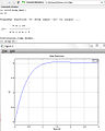 Step response

Now, let's look at the modern, state-space approach. If we have the matrices A, B, C and D, we can plug these into the step function, as shown:
step(A, B, C, D);
or, we can optionally include a vector for time, t:
step(A, B, C, D, t);
Again, if we supply results on the left-hand side of the equation, MATLAB will not automatically produce a plot for us.
If we didn't get an automatic plot, and we want to produce our own, we type:
[y, x, t] = step(NUM, DEN, t);
And then we can create a graph using the plot command:
plot(t, y);
y is the output magnitude of the step response, while x is the internal state of the system from the state-space equations:
Classical ↔ Modern
MATLAB contains features that can be used to automatically convert to the state-space representation from the Laplace representation. This function, tf2ss, is used as follows:
[A, B, C, D] = tf2ss(NUM, DEN);
Where NUM and DEN are the coefficient vectors of the numerator and denominator of the transfer function, respectively.
In a similar vein, we can convert from the Laplace domain back to the state-space representation using the ss2tf function, as such:
[NUM, DEN] = ss2tf(A, B, C, D);
Or, if we have more than one input in a vector u, we can write it as follows:
[NUM, DEN] = ss2tf(A, B, C, D, u);
The u parameter must be provided when our system has more than one input, but it does not need to be provided if we have only 1 input. This form of the equation produces a transfer function for each separate input. NUM and DEN become 2-D matricies, with each row being the coefficients for each different input.
z-Domain Digital Filters
Let us now consider a digital system with the following generic transfer function in the Z domain:

Where n(z) and d(z) are the numerator and denominator polynomials of the transfer function, respectively. The filter command can be used to apply an input vector x to the filter. The output, y, can be obtained from the following code:
y = filter(n, d, x);
The word "filter" may be a bit of a misnomer in this case, but the fact remains that this is the method to apply an input to a digital system. Once we have the output magnitude vector, we can plot it using our plot command:
plot(y);
To get the step response of the digital system, we must first create a step function using the ones command:
u = ones(1, N);
Where N is the number of samples that we want to take in our digital system (not to be confused with "n", our numerator coefficient). Once we have produced our unit step function, we can pass this function through our digital filter as such:
y = filter(n, d, u);
And we can plot y:
plot(y);
State-Space Digital Filters
Likewise, we can analyze a digital system in the state-space representation. If we have the following digital state relationship:
We can convert automatically to the pulse response using the ss2tf function, that we used above:
[NUM, DEN] = ss2tf(A, B, C, D);
Then, we can filter it with our prepared unit-step sequence vector, u:
y = filter(num, den, u)
this will give us the step response of the digital system in the state-space representation.
Root Locus Plots
MATLAB supplies a useful, automatic tool for generating the root-locus graph from a transfer function: the rlocus command. In the transfer function domain, or the state space domain respectively, we have the following uses of the function:
rlocus(num, den);
And:
rlocus(A, B, C, D);
These functions will automatically produce root-locus graphs of the system. However, if we provide left-hand parameters:
[r, K] = rlocus(num, den);
Or:
[r, K] = rlocus(A, B, C, D);
The function won't produce a graph automatically, and you will need to produce one yourself. There is also an optional additional parameter for gain, K, that can be supplied:
rlocus(num, den, K);
Or:
rlocus(A, B, C, D, K);
If K is not supplied, MATLAB will supply an automatic gain value for you.
Once we have our values [r, K], we can plot a root locus:
plot(r);
The rlocus command cannot be used with MIMO systems, so if your system is a MIMO system, you must separate out your coefficient matrices to isolate each separate Input-output pair, and graph each individually.
Here is a sample screenshot:
-
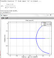 root-locus

Digital Root-Locus
Creating a root-locus diagram for a digital system is exactly the same as it is for a continuous system. The only difference is the interpretation of the results, because the stability region for digital systems is different from the stability region for continuous systems. The same rlocus function can be used, in the same manner as is used above.
Bode Plots
MATLAB also offers a number of tools for examining the frequency response characteristics of a system, both using Bode plots, and using Nyquist charts. To construct a Bode plot from a transfer function, we use the following command:
[mag, phase, omega] = bode(NUM, DEN, omega);
Or:
[mag, phase, omega] = bode(A, B, C, D, u, omega);
Where "omega" is the frequency vector where the magnitude and phase response points are analyzed. If we want to convert the magnitude data into decibels, we can use the following conversion:
magdb = 20 * log10(mag);
This conversion should be known well enough by now that it doesn't require explanation.
When talking about Bode plots in decibels, it makes the most sense (and is the most common occurrence) to also use a logarithmic frequency scale. To create such a logarithmic sequence in omega, we use the logspace command, as such:
omega = logspace(a, b, n);
This command produces n points, spaced logarithmicly, from up to .


If we use the bode command without left-hand arguments, MATLAB will produce a graph of the bode phase and magnitude plots automatically.
The bode command, if used with a MIMO system, will use subplots to produce all the input-output relationship graphs on a single plot window. for a system with multiple inputs and multiple outputs, this can become difficult to see clearly. In these cases, it is typically better to separate out your coefficient matrices to isolate each individual input-output pair.
Here is a sample screenshot:
-
 Bode plot (Frequency response)

Nyquist Plots
In addition to the bode plots, we can create nyquist charts by using the nyquist command. The nyquist command operates in a similar manner to the bode command (and other commands that we have used so far):
[real, imag, omega] = nyquist(NUM, DEN, omega);
Or:
[real, imag, omega] = nyquist(A, B, C, D, u, omega);
Here, "real" and "imag" are vectors that contain the real and imaginary parts of each point of the nyquist diagram. If we don't supply the right-hand arguments, the nyquist command automatically produces a nyquist plot for us.
Like the bode command, the nyquist command will use subplots to display the input-output relations of MIMO systems on a single plot window. If there are multiple input-output pairs, it can be difficult to see the individual graphs.
Here is a sample screenshot:
-
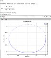 Nyquist plot

Lyapunov Equations
Controllability
A controllability matrix can be constructed using the ctrb command. The controllability gramian can be constructed using the gram command.
Observability
An observability matrix can be constructed using the command obsv
Empirical Gramians
Empirical gramians can be computed for linear and also nonlinear control systems. The empirical gramian framework emgr allows the computation of the controllability, observability and cross gramian; it is compatible with MATLAB and OCTAVE and does not require the control systems toolbox.
Further reading
- Ogata, Katsuhiko, "Solving Control Engineering Problems with MATLAB", Prentice Hall, New Jersey, 1994. ISBN 0130459070
- MATLAB Programming.
- http://octave.sourceforge.net/
- MATLAB Category on ControlTheoryPro.com
- Empirical Gramian Framework
Glossary
Resources
Licensing
1) Glossary
2) List of Equations
3) Resources and Bibliography
4) Licensing
5) GNU Free Documentation License
Glossary and List of Equations
The following is a listing of some of the most important terms from the book, along with a short definition or description.
A, B, C
- Acceleration Error
- The amount of steady state error of the system when stimulated by a unit parabolic input.
- Acceleration Error Constant
- A system metric that determines that amount of acceleration error in the system.
- Adaptive Control
- A branch of control theory where controller systems are able to change their response characteristics over time, as the input characteristics to the system change.
- Adaptive Gain
- when control gain is varied depending on system state or condition, such as a disturbance
- Additivity
- A system is additive if a sum of inputs results in a sum of outputs.
- Analog System
- A system that is continuous in time and magnitude.
- ARMA
- Autoregressive Moving Average, see [1]
- ATO
- Analog Timed Output. Control loop output is correlated to a timed contact closure.
- A/M
- Auto-Manual. Control modes, where auto typically means output is computer-driven, calculated while manual can be field-driven or merely using a static setpoint.
- Bilinear Transform
- a variant of the Z-transform, see [2]
- Block Diagram
- A visual way to represent a system that displays individual system components as boxes, and connections between systems as arrows.
- Bode Plots
- A set of two graphs, a "magnitude" and a "phase" graph, that are both plotted on log scale paper. The magnitude graph is plotted in decibels versus frequency, and the phase graph is plotted in degrees versus frequency. Used to analyze the frequency characteristics of the system.
- Bounded Input, Bounded Output
- BIBO. If the input to the system is finite, then the output must also be finite. A condition for stability.
- Cascade
- When the output of a control loop is fed to/from another loop.
- Causal
- A system whose output does not depend on future inputs. All physical systems must be causal.
- Classical Approach
- See Classical Controls.
- Classical Controls
- A control methodology that uses the transform domain to analyze and manipulate the Input-Output characteristics of a system.
- Closed Loop
- a controlled system using feedback or feedforward
- Compensator
- A Control System that augments the shortcomings of another system.
- Condition Number
- Conditional Stability
- A system with variable gain is conditionally stable if it is BIBO stable for certain values of gain, but not BIBO stable for other values of gain.
- Continuous-Time
- A system or signal that is defined at all points t.
- Control Rate
- the rate at which control is computed and any appropriate output sent. Lower bound is sample rate.
- Control System
- A system or device that manages the behavior of another system or device.
- Controller
- See Control System.
- Convolution
- A complex operation on functions defined by the integral of the two functions multiplied together, and time-shifted.
- Convolution Integral
- The integral form of the convolution operation.
- CQI
- Control Quality Index, , 1 being ideal.
- CV
- Controlled variable
![{\displaystyle =1-abs(PV-SP)/max[PVmax-SP,SP-PVmin]}](https://wikimedia.org/api/rest_v1/media/math/render/svg/2a34d47acce2287268821b38f7a46ad1f4debaf7)
D, E, F
- Damping Ratio
- A constant that determines the damping properties of a system.
- Deadtime
- time shift between the output change and the related effect (typ. at least one control sample). One sees "Lag" used for this action sometimes.
- Digital
- A system that is both discrete-time, and quantized.
- Direct action
- target output increase is required to bring the process variable (PV) to setpoint (SP) when PV is below SP. Thus, PV increases with output increase directly.
- Discrete magnitude
- See quantized.
- Discrete time
- A system or signal that is only defined at specific points in time.
- Distributed
- A system is distributed if it has both an infinite number of states, and an infinite number of state variables. See Lumped.
- Dynamic
- A system is called dynamic if it doesn't have memory. See Instantaneous, Memory.
- Eigenvalues
- Solutions to the characteristic equation of a matrix. If the matrix is itself a function of time, the eigenvalues might be functions of time. In this case, they are frequently called eigenfunctions.
- Eigenvectors
- The nullspace vectors of the characteristic equation for particular eigenvalues. Used to determine state-transitions, among other things. See [3]
- Euler's Formula
- An equation that relates complex exponentials to complex sinusoids.
- Exponential Weighted Average (EWA)
- Apportions fractional weight to new and existing data to form a working average. Example EWA=0.70*EWA+0.30*latest, see Filtering.
- External Description
- A description of a system that relates the input of the system to the output, without explicitly accounting for the internal states of the system.
- Feedback
- The output of the system is passed through some sort of processing unit H, and that result is fed into the plant as an input.
- Feedforward
- whwn apriori knowledge is used to forecast at least part of the control response.
- Filtering (noise)
- Use of signal smoothing techniques to reject undesirable components like noise. Can be as simple as using exponential weighted averaging on the input.
- Final Value Theorem
- A theorem that allows the steady-state value of a system to be determined from the transfer function.
- FOH
- First order hold
- Frequency Response
- The response of a system to sinusoids of different frequencies. The Fourier Transform of the impulse response.
- Fourier Transform
- An integral transform, similar to the Laplace Transform, that analyzes the frequency characteristics of a system.
See [4]
G, H, I
- Game Theory
- A branch of study that is related to control engineering, and especially optimal control. Multiple competing entities, or "players" attempt to minimize their own cost, and maximize the cost of the opponents.
- Gain
- A constant multiplier in a system that is typically implemented as an amplifier or attenuator. Gain can be changed, but is typically not a function of time. Adaptive control can use time-adaptive gains that change with time.
- General Description
- An external description of a system that relates the system output to the system input, the system response, and a time constant through integration.
- Hendrik Wade Bode
- Electrical Engineer, did work in control theory and communications. Is primarily remembered in control engineering for his introduction of the bode plot.
- Harry Nyquist
- Electrical Engineer, did extensive work in controls and information theory. Is remembered in this book primarily for his introduction of the Nyquist Stability Criterion.
- Homogeniety
- Property of a system whose scaled input results in an equally scaled output.
- Hybrid Systems
- Systems which have both analog and digital components.
- Impulse
- A function denoted δ(t), that is the derivative of the unit step.
- Impulse Response
- The system output when the system is stimulated by an impulse input. The Inverse Laplace Transform of the transfer function of the system.
- Initial Conditions
- The conditions of the system at time , where t0 is the first time the system is stimulated.
- Initial Value Theorem
- A theorem that allows the initial conditions of the system to be determined from the Transfer function.
- Input-Output Description
- See external description.
- Instantaneous
- A system is instantaneous if the system doesn't have memory, and if the current output of the system is only dependent on the current input. See Dynamic, Memory.
- Integrated Absolute Error (IAE)
- absolute error (ideal vs actual performance) is integrated over the analysis period.
- Integrated Squared Error (ISE)
- squared error (ideal vs actual performance) is integrated over the analysis period.
- Integrators
- A system pole at the origin of the S-plane. Has the effect of integrating the system input.
- Inverse Fourier Transform
- An integral transform that converts a function from the frequency domain into the time-domain.
- Inverse Laplace Transform
- An integral transform that converts a function from the S-domain into the time-domain.
- Inverse Z-Transform
- An integral transform that converts a function from the Z-domain into the discrete time domain.

J, K, L
- Lag
- The observed process impact from an output is slower than the control rate.
- Laplace Transform
- An integral transform that converts a function from the time domain into a complex frequency domain.
- Laplace Transform Domain
- A complex domain where the Laplace Transform of a function is graphed. The imaginary part of s is plotted along the vertical axis, and the real part of s is plotted along the horizontal axis.
- Left Eigenvectors
- Left-hand nullspace solutions to the characteristic equation of a matrix for given eigenvalues. The rows of the inverse transition matrix.
- Linear
- A system that satisfies the superposition principle. See Additive and Homogeneous.
- Linear Time-Invariant
- LTI. See Linear, and Time-Invariant.
- Low Clamp
- User-applied lower bound on control output signal.
- L/R
- Local/Remote operation.
- LQR
- Linear Quadratic Regulator.
- Lumped
- A system with a finite number of states, or a finite number of state variables.
M, N, O
- Magnitude
- the gain component of frequency response. This is often all that is considered in saying a discrete filter's response is well matched to the analog's. It is the DC gain at 0 frequency.
- Marginal Stability
- A system has an oscillatory response, as determined by having imaginary poles or imaginary eigenvalues.
- Mason's Rule
- see [5]
- MATLAB
- Commercial software having a Control Systems toolbox. Also see Octave.
- Memory
- A system has memory if its current output is dependent on previous and current inputs.
- MFAC
- Model Free Adaptive Control.
- MIMO
- A system with multiple inputs and multiple outputs.
- Modern Approach
- see modern controls
- Modern Controls
- A control methodology that uses the state-space representation to analyze and manipulate the Internal Description of a system.
- Modified Z-Transform
- A version of the Z-Transform, expanded to allow for an arbitrary processing delay.
- MPC
- Model Predictive Control.
- MRAC
- Model Reference Adaptive Control.
- MV
- can denote Manipulated variable or Measured variable (not the same)
- Natural Frequency
- The fundamental frequency of the system, the frequency for which the system's frequency response is largest.
- Negative Feedback
- A feedback system where the output signal is subtracted from the input signal, and the difference is input to the plant.
- The Nyquist Criteria
- A necessary and sufficient condition of stability that can be derived from Bode plots.
- Nonlinear Control
- A branch of control engineering that deals exclusively with non-linear systems. We do not cover nonlinear systems in this book.
- OCTAVE
- Open-source software having a Control Systems toolbox. Also see MATLAB.
- Offset
- The discrepancy between desired and actual value after settling. P-only control can give offset.
- Oliver Heaviside
- Electrical Engineer, Introduced the Laplace Transform as a tool for control engineering.
- Open Loop
- when the system is not closed, its behavior has a free-running component rather than controlled
- Optimal Control
- A branch of control engineering that deals with the minimization of system cost, or maximization of system performance.
- Order
- The order of a polynomial is the highest exponent of the independent variable in that exponent. The order of a system is the order of the Transfer Function's denominator polynomial.
- Output equation
- An equation that relates the current system input, and the current system state to the current system output.
- Overshoot
- measures the extent of system response against desired (setpoint tracking).
P, Q, R
- Parabolic
- A parabolic input is defined by the equation.
- Partial Fraction Expansion
- A method by which a complex fraction is decomposed into a sum of simple fractions.
- Percent Overshoot
- PO, the amount by which the step response overshoots the reference value, in percentage of the reference value.
- Phase
- the directional component of frequency response, not typically well-matched between a discrete filter equivalent to the analog version, especially as frequency approaches the Nyquist limit. The final value in the limit drives system stability, and stems from the poles and zeros of the characteristic equation.
- PID
- Proportional-Integral-Derivative
- Plant
- A central system which has been provided, and must be analyzed or controlled.
- PLC
- Programmable Logic Controller
- Pole
- A value for s that causes the denominator of the transfer function to become zero, and therefore causes the transfer function itself to approach infinity.
- Pole-Zero Form
- The transfer function is factored so that the locations of all the poles and zeros are clearly evident.
- Position Error
- The amount of steady-state error of a system stimulated by a unit step input.
- Position Error Constant
- A constant that determines the position error of a system.
- Positive Feedback
- A feedback system where the system output is added to the system input, and the sum is input into the plant.
- PSD
- The power spectral density which shows the distribution of power in the spectrum of a particular signal.
- Pulse Response
- The response of a digital system to a unit step input, in terms of the transfer matrix.
- PV
- Process variable

- Quantized
- A system is quantized if it can only output certain discrete values.
- Quarter-decay
- the time or number of control rates required for process overshoot to be limited to within 1/4 of the maximum peak overshoot (PO) after a SP change. If the PO is 25% at sample time N, this would be time N+k when subsequent PV remains < SP*1.0625, presuming the process is settling.
- Raise-Lower
- Output type that works from present position rather than as a completely new computed spanned output. For R/L, the % change should be applied to the working clamps i.e. 5%(hi clamp-lo clamp).
- Ramp
- A ramp is defined by the function .
- Reconstructors
- A system that converts a digital signal into an analog signal.
- Reference Value
- The target input value of a feedback system.
- Relaxed
- A system is relaxed if the initial conditions are zero.
- Reverse action
- target output decrease is required to bring the process variable (PV) to setpoint (SP) when PV is below SP. Thus, PV decreases with output increase.
- Rise Time
- The amount of time it takes for the step response of the system to reach within a certain range of the reference value. Typically, this range is 80%.
- Robust Control
- A branch of control engineering that deals with systems subject to external and internal noise and disruptions.

S, T, U, V
- Samplers
- A system that converts an analog signal into a digital signal.
- Sampled-Data Systems
- See Hybrid Systems'.
- Sampling Time
- In a discrete system, the sampling time is the amount of time between samples. Reflects the lower bound for Control rate.
- SCADA
- Supervisory Control and Data Acquisition.
- S-Domain
- The domain of the Laplace Transform of a signal or system.
- Second-order System;
- Settling Time
- The amount of time it takes for the system's oscillatory response to be damped to within a certain band of the steady-state value. That band is typically 10%.
- Signal Flow Diagram
- A method of visually representing a system, using arrows to represent the direction of signals in the system.
- SISO
- Single input, single output.
- Span
- the designed operation region of the item,=high range-low range. Working span can be smaller if output clamps are used.
- Stability
- Typically "BIBO Stability", a system with a well-behaved input will result in a well-behaved output. "Well-behaved" in this sense is arbitrary.
- Star Transform
- A version of the Laplace Transform that acts on discrete signals. This transform is implemented as an infinite sum.
- State Equation
- An equation that relates the future states of a system with the current state and the current system input.
- State Transition Matrix:A coefficient matrix, or a matrix function that relates how the system state changes in response to the system input. In time-invariant systems, the state-transition matrix is the matrix exponential of the system matrix.
- State-Space Equations
- A set of equations, typically written in matrix form, that relates the input, the system state, and the output. Consists of the state equation and the output equation. See [6]
- State-Variable
- A vector that describes the internal state of the system.
- Stability
- The system output cannot approach infinity as time approaches infinity. See BIBO, Lyapunov Stability.
- Step Response
- The response of a system when stimulated by a unit-step input. A unit step is a setpoint change for setpoint tracking.
- Steady State
- The output value of the system as time approaches infinity.
- Steady State Error
- At steady state, the amount by which the system output differs from the reference value.
- Superposition
- A system satisfies the condition of superposition if it is both additive and homogeneous.
- System Identification
- method of trying to identify the system characterization , typically through least squares analysis of input,output and noise data vectors. May use ARMA type framework.
- System Type
- The number of ideal integrators in the system.
- Time-Invariant
- A system is time-invariant if an input time-shifted by an arbitrary delay produces an output shifted by that same delay.
- Transfer Function
- The ratio of the system output to its input, in the S-domain. The Laplace Transform of the function's impulse response.
- Transfer Function Matrix:The Laplace transform of the state-space equations of a system, that provides an external description of a MIMO system.
- Uniform Stability
- Also "Uniform BIBO Stability", a system where an input signal in the range [0, 1] results in a finite output from the initial time until infinite time. See [7].
- Unit Step
- An input defined by . Practically, a setpoint change.
- Unity Feedback
- A feedback system where the feedback loop element H has a transfer function of 1.
- Velocity Error
- The amount of steady-state error when the system is stimulated by a ramp input.
- Velocity Error Constant
- A constant that determines that amount of velocity error in a system.
W, X, Y, Z
- W-plane
- Reference plane used in the bilinear transform.
- Wind-up
- when the numerics of computed control adjustment can "wind-up", yielding control correction with an inappropriate component unless prevented. An example is the "I" contribution of PID if output has been disconnected during PID calculation
- Zero
- A value for s that causes the numerator of the transfer function to become zero, and therefore causes the transfer function itself to become zero.
- Zero Input Response
- The response of a system with zero external input. Relies only on the value of the system state to produce output.
- Zero State Response
- The response of the system with zero system state. The output of the system depends only on the system input.
- ZOH
- Zero order hold.
- Z-Transform
- An integral transform that is related to the Laplace transform through a change of variables. The Z-Transform is used primarily with digital systems. See [8]
List of Equations
The following is a list of the important equations from the text, arranged by subject. For more information about these equations, including the meaning of each variable and symbol, the uses of these functions, or the derivations of these equations, see the relevant pages in the main text.
Fundamental Equations
[Euler's Formula]

[Convolution]

[Convolution Theorem]
[Characteristic Equation]
[Decibels]
Basic Inputs
[Unit Step Function]
[Unit Ramp Function]
[Unit Parabolic Function]
Error Constants
[Position Error Constant]
[Velocity Error Constant]
[Acceleration Error Constant]
System Descriptions
[General System Description]

[Convolution Description]
[Transfer Function Description]
[State-Space Equations]
[Transfer Matrix]
[Transfer Matrix Description]
[Mason's Rule]
Feedback Loops
[Closed-Loop Transfer Function]

[Open-Loop Transfer Function]
[Characteristic Equation]

Transforms
[Laplace Transform]
![{\displaystyle F(s)={\mathcal {L}}[f(t)]=\int _{0}^{\infty }f(t)e^{-st}dt}](https://wikimedia.org/api/rest_v1/media/math/render/svg/0c38c98774feaf400f8af0dab5f8aed8aed5d06f)
[Inverse Laplace Transform]

[Fourier Transform]
[Inverse Fourier Transform]
[Star Transform]
![{\displaystyle F^{*}(s)={\mathcal {L}}^{*}[f(t)]=\sum _{i=0}^{\infty }f(iT)e^{-siT}}](https://wikimedia.org/api/rest_v1/media/math/render/svg/30b1617367f1700032ffd3f5b8720159699648ed)
[Z Transform]
![{\displaystyle X(z)={\mathcal {Z}}\left\{x[n]\right\}=\sum _{i=-\infty }^{\infty }x[n]z^{-n}}](https://wikimedia.org/api/rest_v1/media/math/render/svg/af2109d64c2b69a9a5104d600e08fc9b4267360b)
[Inverse Z Transform]
[Modified Z Transform]
Transform Theorems
[Final Value Theorem]

![{\displaystyle x[\infty ]=\lim _{z\to 1}(z-1)X(z)}](https://wikimedia.org/api/rest_v1/media/math/render/svg/30f34e1769d16e186e49651f66f4401a8c589b3e)
[Initial Value Theorem]
State-Space Methods
[General State Equation Solution]

![{\displaystyle x[n]=A^{n}x[0]+\sum _{m=0}^{n-1}A^{n-1-m}Bu[n]}](https://wikimedia.org/api/rest_v1/media/math/render/svg/37dfa3802c72fcf32ac7e379d52ae691154fad04)
[General Output Equation Solution]

![{\displaystyle y[n]=CA^{n}x[0]+\sum _{m=0}^{n-1}CA^{n-1-m}Bu[n]+Du[n]}](https://wikimedia.org/api/rest_v1/media/math/render/svg/08c5007961a18ea382ac3c879331fb4e87873560)
[Time-Variant General Solution]

![{\displaystyle x[n]=\phi [n,n_{0}]x[t_{0}]+\sum _{m=n_{0}}^{n}\phi [n,m+1]B[m]u[m]}](https://wikimedia.org/api/rest_v1/media/math/render/svg/44156ca6ba03d51f16817e0cd51292ca38563a80)
[Impulse Response Matrix]

![{\displaystyle G[n]=\left\{{\begin{matrix}CA^{k-1}N&{\mbox{ if }}k>0\\0&{\mbox{ if }}k\leq 0\end{matrix}}\right.}](https://wikimedia.org/api/rest_v1/media/math/render/svg/90177e0e9300b0985968117dde9fa1f3a5aec597)
Root Locus
[The Magnitude Equation]
[The Angle Equation]
[Number of Asymptotes]
[Angle of Asymptotes]
[Origin of Asymptotes]
[Breakaway Point Locations]
- or


Lyapunov Stability
[Lyapunov Equation]
Controllers and Compensators
[PID]
Resources and Further Reading
Wikibooks
A number of wikibooks exist on topics that are (a) prerequisites to this book (b) companion pieces to and references for this book, and (c) of further interest to people who have completed reading this book. Below will be a listing of such books, ordered according to the categories listed above.
Prerequisite Books
- Linear algebra
- Linear Algebra with Differential Equations
- Complex Numbers
- Calculus
- Signals and Systems
Companion Books
Books for Further Reading
Wikiversity
The Wikiversity project also contains a number of collaborative learning efforts in the field of control systems, and related subjects. As best as possible, we will attempt to list those efforts here:
Wikiversity is also a place to host learning materials, such as assignments, tests, and reading plans. It is the goal of the authors of this book to create such materials for use in conjunction with this book. As such materials are added to wikiversity, they will be referenced here.
Wikipedia
There are a number of Wikipedia articles on the topics covered in this book, and those articles will be linked to from the appropriate pages of this book. However, some of the articles that are of general use to the book are:
A complete listing of all Wikipedia articles related to this topic can be found at:
Software
Root Locus
Root-Locus is a free program that was used to create several of the images in this book. That software can be obtained from the following web address:
Explicit permission has been granted by the author of the program to include screenshots on wikibooks. Images generated from the Root-Locus program should be included in Category:Root Locus Images, and appropriately tagged as a screenshot of a free software program.
MATLAB
MATLAB, Simulink, the Control Systems Toolbox and the Symbolic Toolbox are trademarks of The MathWorks, Inc. Other product or brand names are trademarks or registered trademarks of their respective holders. For more information about MATLAB, or to purchase a copy, visit:
For information about the proper way to refer to MATLAB, please see:
All MATLAB code appearing in this book has been released under the terms of the GFDL by the respective authors. All screenshots, graphs, and images relating to MATLAB have been produced in Octave, with changes to the original MATLAB code made as necessary.
Octave
Octave is a free open-source alternative program to MATLAB. Octave utilizes a scripting language that is very similar to that of MATLAB, although there are several differences. Most of the basic examples described in this book will work equally well in MATLAB or Octave, with no changes or only minor changes. For more information, or to download a copy of Octave, visit:
Commercial Vendors
The following are some common vendors of control-related hardware and software. These links are for personal interest only, and do not constitute an official endorsement of the companies by Wikibooks.
External Publications
The following books and resources were used as reference works in the creation of this wikibook (books listed in alphabetical order).
- Brogan, William L, Modern Control Theory, 3rd Edition, 1991. ISBN 0135897637
- Chen, Chi-Tsong, Linear System Theory and Design, 3rd Edition, 1999. ISBN 0195117778
- Dorf and Bishop, Modern Control Systems, 10th Edition, Prentice Hall, 2005. ISBN 0131277650
- Hamming, Richard, Numerical Methods for Scientists and Engineers, 2nd edition, Dover, 1987. ISBN 0486652416
- Kalman, R. E., When is a linear control system optimal, ASME Transactions, Journal of Basic Engineering, 1964
- Kalman, R. E., On the General Theory of Control Systems, IRE Transactions on Automatic Control, Volume 4, Issue 3, p110, 1959. ISSN 0096199X
- Ogata, Katsuhiko, Solving Control Engineering Problems with MATLAB, Prentice Hall, New Jersey, 1994. ISBN 0130459070
- Phillips and Nagle, Digital Control System Analysis and Design, 3rd Edition, Prentice Hall, 1995. ISBN 013309832X
The following books and resources are suitable for further reading.
- DiStefano, Stubberud, Williams, Schaum's Outline Series Feedback and Control Systems, 2nd Edition, 1997. ISBN 0070170479
- Franklin, Powell, Workman, Digital Control of Dynamic Systems, 3rd Edition, 1997. ISBN 9780201820546
- Brosilow, Joseph, Techniques of Model-Based Control, 2002. ISBN 013028078X
External Resources
- IEEE Control Systems Society
- ControlTheoryPro.com A place for controls theory, application, and modeling help.
- University of Michigan Chemical Engineering Process Dynamics and Controls Open Textbook
Licensing
License
The text of this wikibook is released under the terms of the GNU Free Documentation License version 1.2. The particular version of that license that is being used can be found at:
The text of that license will also be appended to the end of the printable version of this wikibook.
Images used in this document may not be released under the GFDL, and the licenses used with each image in this book will be listed in a table below. Some contributors may cross-license their contributions under the GFDL and another compatible license. Some contributions have been released into the public domain.
Images
The individual images used in this wikibook are released under a variety of different licenses, including the GFDL, and Creative-Commons licenses. Some images have been released into the public domain. The following table will list the images used in this book, along with the license under which the image is released, and any additional information about the images that is needed under the terms of the applicable licenses.
.jpg)
Authors
The authors of this text can list themselves below. Authors should be listed in alphabetical order by first name (if a real name is used), or by username. This is not a canonical list.
The usernames of additional contributors, as well as the size and scope of the contributions made by the authors listed above can be found in the history records of the individual pages on the Wikibooks website. Those history pages satisfy the attribution requirement of the GFDL, and any lists of authors that appear here or anywhere else do not count as legal attribution under the terms of that license.
Child Versions
The Control Systems wikibook is offered with a number of child versions, which represent subsets of the material available in the parent book. Because certain chapters are omitted from the child versions, some of the images listed above may not be present, and some of the authors listed above may not have made any contributions to some printed and distributed versions of this text.
License: GFDL
As of July 15, 2009 Wikibooks has moved to a dual-licensing system that supersedes the previous GFDL only licensing. In short, this means that text licensed under the GFDL only can no longer be imported to Wikibooks, retroactive to 1 November 2008. Additionally, Wikibooks text might or might not now be exportable under the GFDL depending on whether or not any content was added and not removed since July 15. |
Version 1.3, 3 November 2008 Copyright (C) 2000, 2001, 2002, 2007, 2008 Free Software Foundation, Inc. <http://fsf.org/>
Everyone is permitted to copy and distribute verbatim copies of this license document, but changing it is not allowed.
0. PREAMBLE
The purpose of this License is to make a manual, textbook, or other functional and useful document "free" in the sense of freedom: to assure everyone the effective freedom to copy and redistribute it, with or without modifying it, either commercially or noncommercially. Secondarily, this License preserves for the author and publisher a way to get credit for their work, while not being considered responsible for modifications made by others.
This License is a kind of "copyleft", which means that derivative works of the document must themselves be free in the same sense. It complements the GNU General Public License, which is a copyleft license designed for free software.
We have designed this License in order to use it for manuals for free software, because free software needs free documentation: a free program should come with manuals providing the same freedoms that the software does. But this License is not limited to software manuals; it can be used for any textual work, regardless of subject matter or whether it is published as a printed book. We recommend this License principally for works whose purpose is instruction or reference.
1. APPLICABILITY AND DEFINITIONS
This License applies to any manual or other work, in any medium, that contains a notice placed by the copyright holder saying it can be distributed under the terms of this License. Such a notice grants a world-wide, royalty-free license, unlimited in duration, to use that work under the conditions stated herein. The "Document", below, refers to any such manual or work. Any member of the public is a licensee, and is addressed as "you". You accept the license if you copy, modify or distribute the work in a way requiring permission under copyright law.
A "Modified Version" of the Document means any work containing the Document or a portion of it, either copied verbatim, or with modifications and/or translated into another language.
A "Secondary Section" is a named appendix or a front-matter section of the Document that deals exclusively with the relationship of the publishers or authors of the Document to the Document's overall subject (or to related matters) and contains nothing that could fall directly within that overall subject. (Thus, if the Document is in part a textbook of mathematics, a Secondary Section may not explain any mathematics.) The relationship could be a matter of historical connection with the subject or with related matters, or of legal, commercial, philosophical, ethical or political position regarding them.
The "Invariant Sections" are certain Secondary Sections whose titles are designated, as being those of Invariant Sections, in the notice that says that the Document is released under this License. If a section does not fit the above definition of Secondary then it is not allowed to be designated as Invariant. The Document may contain zero Invariant Sections. If the Document does not identify any Invariant Sections then there are none.
The "Cover Texts" are certain short passages of text that are listed, as Front-Cover Texts or Back-Cover Texts, in the notice that says that the Document is released under this License. A Front-Cover Text may be at most 5 words, and a Back-Cover Text may be at most 25 words.
A "Transparent" copy of the Document means a machine-readable copy, represented in a format whose specification is available to the general public, that is suitable for revising the document straightforwardly with generic text editors or (for images composed of pixels) generic paint programs or (for drawings) some widely available drawing editor, and that is suitable for input to text formatters or for automatic translation to a variety of formats suitable for input to text formatters. A copy made in an otherwise Transparent file format whose markup, or absence of markup, has been arranged to thwart or discourage subsequent modification by readers is not Transparent. An image format is not Transparent if used for any substantial amount of text. A copy that is not "Transparent" is called "Opaque".
Examples of suitable formats for Transparent copies include plain ASCII without markup, Texinfo input format, LaTeX input format, SGML or XML using a publicly available DTD, and standard-conforming simple HTML, PostScript or PDF designed for human modification. Examples of transparent image formats include PNG, XCF and JPG. Opaque formats include proprietary formats that can be read and edited only by proprietary word processors, SGML or XML for which the DTD and/or processing tools are not generally available, and the machine-generated HTML, PostScript or PDF produced by some word processors for output purposes only.
The "Title Page" means, for a printed book, the title page itself, plus such following pages as are needed to hold, legibly, the material this License requires to appear in the title page. For works in formats which do not have any title page as such, "Title Page" means the text near the most prominent appearance of the work's title, preceding the beginning of the body of the text.
The "publisher" means any person or entity that distributes copies of the Document to the public.
A section "Entitled XYZ" means a named subunit of the Document whose title either is precisely XYZ or contains XYZ in parentheses following text that translates XYZ in another language. (Here XYZ stands for a specific section name mentioned below, such as "Acknowledgements", "Dedications", "Endorsements", or "History".) To "Preserve the Title" of such a section when you modify the Document means that it remains a section "Entitled XYZ" according to this definition.
The Document may include Warranty Disclaimers next to the notice which states that this License applies to the Document. These Warranty Disclaimers are considered to be included by reference in this License, but only as regards disclaiming warranties: any other implication that these Warranty Disclaimers may have is void and has no effect on the meaning of this License.
2. VERBATIM COPYING
You may copy and distribute the Document in any medium, either commercially or noncommercially, provided that this License, the copyright notices, and the license notice saying this License applies to the Document are reproduced in all copies, and that you add no other conditions whatsoever to those of this License. You may not use technical measures to obstruct or control the reading or further copying of the copies you make or distribute. However, you may accept compensation in exchange for copies. If you distribute a large enough number of copies you must also follow the conditions in section 3.
You may also lend copies, under the same conditions stated above, and you may publicly display copies.
3. COPYING IN QUANTITY
If you publish printed copies (or copies in media that commonly have printed covers) of the Document, numbering more than 100, and the Document's license notice requires Cover Texts, you must enclose the copies in covers that carry, clearly and legibly, all these Cover Texts: Front-Cover Texts on the front cover, and Back-Cover Texts on the back cover. Both covers must also clearly and legibly identify you as the publisher of these copies. The front cover must present the full title with all words of the title equally prominent and visible. You may add other material on the covers in addition. Copying with changes limited to the covers, as long as they preserve the title of the Document and satisfy these conditions, can be treated as verbatim copying in other respects.
If the required texts for either cover are too voluminous to fit legibly, you should put the first ones listed (as many as fit reasonably) on the actual cover, and continue the rest onto adjacent pages.
If you publish or distribute Opaque copies of the Document numbering more than 100, you must either include a machine-readable Transparent copy along with each Opaque copy, or state in or with each Opaque copy a computer-network location from which the general network-using public has access to download using public-standard network protocols a complete Transparent copy of the Document, free of added material. If you use the latter option, you must take reasonably prudent steps, when you begin distribution of Opaque copies in quantity, to ensure that this Transparent copy will remain thus accessible at the stated location until at least one year after the last time you distribute an Opaque copy (directly or through your agents or retailers) of that edition to the public.
It is requested, but not required, that you contact the authors of the Document well before redistributing any large number of copies, to give them a chance to provide you with an updated version of the Document.
4. MODIFICATIONS
You may copy and distribute a Modified Version of the Document under the conditions of sections 2 and 3 above, provided that you release the Modified Version under precisely this License, with the Modified Version filling the role of the Document, thus licensing distribution and modification of the Modified Version to whoever possesses a copy of it. In addition, you must do these things in the Modified Version:
- Use in the Title Page (and on the covers, if any) a title distinct from that of the Document, and from those of previous versions (which should, if there were any, be listed in the History section of the Document). You may use the same title as a previous version if the original publisher of that version gives permission.
- List on the Title Page, as authors, one or more persons or entities responsible for authorship of the modifications in the Modified Version, together with at least five of the principal authors of the Document (all of its principal authors, if it has fewer than five), unless they release you from this requirement.
- State on the Title page the name of the publisher of the Modified Version, as the publisher.
- Preserve all the copyright notices of the Document.
- Add an appropriate copyright notice for your modifications adjacent to the other copyright notices.
- Include, immediately after the copyright notices, a license notice giving the public permission to use the Modified Version under the terms of this License, in the form shown in the Addendum below.
- Preserve in that license notice the full lists of Invariant Sections and required Cover Texts given in the Document's license notice.
- Include an unaltered copy of this License.
- Preserve the section Entitled "History", Preserve its Title, and add to it an item stating at least the title, year, new authors, and publisher of the Modified Version as given on the Title Page. If there is no section Entitled "History" in the Document, create one stating the title, year, authors, and publisher of the Document as given on its Title Page, then add an item describing the Modified Version as stated in the previous sentence.
- Preserve the network location, if any, given in the Document for public access to a Transparent copy of the Document, and likewise the network locations given in the Document for previous versions it was based on. These may be placed in the "History" section. You may omit a network location for a work that was published at least four years before the Document itself, or if the original publisher of the version it refers to gives permission.
- For any section Entitled "Acknowledgements" or "Dedications", Preserve the Title of the section, and preserve in the section all the substance and tone of each of the contributor acknowledgements and/or dedications given therein.
- Preserve all the Invariant Sections of the Document, unaltered in their text and in their titles. Section numbers or the equivalent are not considered part of the section titles.
- Delete any section Entitled "Endorsements". Such a section may not be included in the Modified version.
- Do not retitle any existing section to be Entitled "Endorsements" or to conflict in title with any Invariant Section.
- Preserve any Warranty Disclaimers.
If the Modified Version includes new front-matter sections or appendices that qualify as Secondary Sections and contain no material copied from the Document, you may at your option designate some or all of these sections as invariant. To do this, add their titles to the list of Invariant Sections in the Modified Version's license notice. These titles must be distinct from any other section titles.
You may add a section Entitled "Endorsements", provided it contains nothing but endorsements of your Modified Version by various parties—for example, statements of peer review or that the text has been approved by an organization as the authoritative definition of a standard.
You may add a passage of up to five words as a Front-Cover Text, and a passage of up to 25 words as a Back-Cover Text, to the end of the list of Cover Texts in the Modified Version. Only one passage of Front-Cover Text and one of Back-Cover Text may be added by (or through arrangements made by) any one entity. If the Document already includes a cover text for the same cover, previously added by you or by arrangement made by the same entity you are acting on behalf of, you may not add another; but you may replace the old one, on explicit permission from the previous publisher that added the old one.
The author(s) and publisher(s) of the Document do not by this License give permission to use their names for publicity for or to assert or imply endorsement of any Modified Version.
5. COMBINING DOCUMENTS
You may combine the Document with other documents released under this License, under the terms defined in section 4 above for modified versions, provided that you include in the combination all of the Invariant Sections of all of the original documents, unmodified, and list them all as Invariant Sections of your combined work in its license notice, and that you preserve all their Warranty Disclaimers.
The combined work need only contain one copy of this License, and multiple identical Invariant Sections may be replaced with a single copy. If there are multiple Invariant Sections with the same name but different contents, make the title of each such section unique by adding at the end of it, in parentheses, the name of the original author or publisher of that section if known, or else a unique number. Make the same adjustment to the section titles in the list of Invariant Sections in the license notice of the combined work.
In the combination, you must combine any sections Entitled "History" in the various original documents, forming one section Entitled "History"; likewise combine any sections Entitled "Acknowledgements", and any sections Entitled "Dedications". You must delete all sections Entitled "Endorsements".
6. COLLECTIONS OF DOCUMENTS
You may make a collection consisting of the Document and other documents released under this License, and replace the individual copies of this License in the various documents with a single copy that is included in the collection, provided that you follow the rules of this License for verbatim copying of each of the documents in all other respects.
You may extract a single document from such a collection, and distribute it individually under this License, provided you insert a copy of this License into the extracted document, and follow this License in all other respects regarding verbatim copying of that document.
7. AGGREGATION WITH INDEPENDENT WORKS
A compilation of the Document or its derivatives with other separate and independent documents or works, in or on a volume of a storage or distribution medium, is called an "aggregate" if the copyright resulting from the compilation is not used to limit the legal rights of the compilation's users beyond what the individual works permit. When the Document is included in an aggregate, this License does not apply to the other works in the aggregate which are not themselves derivative works of the Document.
If the Cover Text requirement of section 3 is applicable to these copies of the Document, then if the Document is less than one half of the entire aggregate, the Document's Cover Texts may be placed on covers that bracket the Document within the aggregate, or the electronic equivalent of covers if the Document is in electronic form. Otherwise they must appear on printed covers that bracket the whole aggregate.
8. TRANSLATION
Translation is considered a kind of modification, so you may distribute translations of the Document under the terms of section 4. Replacing Invariant Sections with translations requires special permission from their copyright holders, but you may include translations of some or all Invariant Sections in addition to the original versions of these Invariant Sections. You may include a translation of this License, and all the license notices in the Document, and any Warranty Disclaimers, provided that you also include the original English version of this License and the original versions of those notices and disclaimers. In case of a disagreement between the translation and the original version of this License or a notice or disclaimer, the original version will prevail.
If a section in the Document is Entitled "Acknowledgements", "Dedications", or "History", the requirement (section 4) to Preserve its Title (section 1) will typically require changing the actual title.
9. TERMINATION
You may not copy, modify, sublicense, or distribute the Document except as expressly provided under this License. Any attempt otherwise to copy, modify, sublicense, or distribute it is void, and will automatically terminate your rights under this License.
However, if you cease all violation of this License, then your license from a particular copyright holder is reinstated (a) provisionally, unless and until the copyright holder explicitly and finally terminates your license, and (b) permanently, if the copyright holder fails to notify you of the violation by some reasonable means prior to 60 days after the cessation.
Moreover, your license from a particular copyright holder is reinstated permanently if the copyright holder notifies you of the violation by some reasonable means, this is the first time you have received notice of violation of this License (for any work) from that copyright holder, and you cure the violation prior to 30 days after your receipt of the notice.
Termination of your rights under this section does not terminate the licenses of parties who have received copies or rights from you under this License. If your rights have been terminated and not permanently reinstated, receipt of a copy of some or all of the same material does not give you any rights to use it.
10. FUTURE REVISIONS OF THIS LICENSE
The Free Software Foundation may publish new, revised versions of the GNU Free Documentation License from time to time. Such new versions will be similar in spirit to the present version, but may differ in detail to address new problems or concerns. See http://www.gnu.org/copyleft/.
Each version of the License is given a distinguishing version number. If the Document specifies that a particular numbered version of this License "or any later version" applies to it, you have the option of following the terms and conditions either of that specified version or of any later version that has been published (not as a draft) by the Free Software Foundation. If the Document does not specify a version number of this License, you may choose any version ever published (not as a draft) by the Free Software Foundation. If the Document specifies that a proxy can decide which future versions of this License can be used, that proxy's public statement of acceptance of a version permanently authorizes you to choose that version for the Document.
11. RELICENSING
"Massive Multiauthor Collaboration Site" (or "MMC Site") means any World Wide Web server that publishes copyrightable works and also provides prominent facilities for anybody to edit those works. A public wiki that anybody can edit is an example of such a server. A "Massive Multiauthor Collaboration" (or "MMC") contained in the site means any set of copyrightable works thus published on the MMC site.
"CC-BY-SA" means the Creative Commons Attribution-Share Alike 3.0 license published by Creative Commons Corporation, a not-for-profit corporation with a principal place of business in San Francisco, California, as well as future copyleft versions of that license published by that same organization.
"Incorporate" means to publish or republish a Document, in whole or in part, as part of another Document.
An MMC is "eligible for relicensing" if it is licensed under this License, and if all works that were first published under this License somewhere other than this MMC, and subsequently incorporated in whole or in part into the MMC, (1) had no cover texts or invariant sections, and (2) were thus incorporated prior to November 1, 2008.
The operator of an MMC Site may republish an MMC contained in the site under CC-BY-SA on the same site at any time before August 1, 2009, provided the MMC is eligible for relicensing.
How to use this License for your documents
To use this License in a document you have written, include a copy of the License in the document and put the following copyright and license notices just after the title page:
- Copyright (c) YEAR YOUR NAME.
- Permission is granted to copy, distribute and/or modify this document
- under the terms of the GNU Free Documentation License, Version 1.3
- or any later version published by the Free Software Foundation;
- with no Invariant Sections, no Front-Cover Texts, and no Back-Cover Texts.
- A copy of the license is included in the section entitled "GNU
- Free Documentation License".
If you have Invariant Sections, Front-Cover Texts and Back-Cover Texts, replace the "with...Texts." line with this:
- with the Invariant Sections being LIST THEIR TITLES, with the
- Front-Cover Texts being LIST, and with the Back-Cover Texts being LIST.
If you have Invariant Sections without Cover Texts, or some other combination of the three, merge those two alternatives to suit the situation.
If your document contains nontrivial examples of program code, we recommend releasing these examples in parallel under your choice of free software license, such as the GNU General Public License, to permit their use in free software.