Control Systems/MATLAB
This page would highly benefit from some screenshots of various systems. Users who have MATLAB or Octave available are highly encouraged to produce some screenshots for the systems here. |
MATLAB
[edit | edit source]MATLAB is a programming language that is specially designed for the manipulation of matrices. Because of its computational power, MATLAB is a tool of choice for many control engineers to design and simulate control systems. This page is going to discuss using MATLAB for control systems design and analysis. MATLAB has a number of plugin modules called "Toolboxes". Nearly all the functions described below are located in the control systems toolbox. If your system has the control systems toolbox installed, you can get more information about the toolbox by typing help control at the MATLAB prompt.
Also, there is an open-source competitor to MATLAB called Octave. Octave is similar to MATLAB, but there are also some differences. This page will focus on MATLAB, but another page could be added to focus on Octave. As of Sept 10th, 2006, all the MATLAB commands listed below have been implemented in GNU octave.
This page will use the {{MATLAB CMD}} template to show MATLAB functions that can be used to perform different tasks.
MATLAB is a copyrighted product produced by The Mathworks. For more information about MATLAB and The Mathworks, see Control Systems/Resources.
Input-Output Isolation
[edit | edit source]In a MIMO system, typically it can be important to isolate a single input-output pair for analysis. Each input corresponds to a single row in the B matrix, and each output corresponds to a single column in the C matrix. For instance, to isolate the 2nd input and the 3rd output, we can create a system:
sys = ss(A, B(:,2), C(3,:), D);
This page will refer to this technique as "input-output isolation".
Step Response
[edit | edit source]First, let's take a look at the classical approach, with the following system:

This system can effectively be modeled as two vectors of coefficients, NUM and DEN:
NUM = [5, 10]
DEN = [1, 4, 5]
Now, we can use the MATLAB step command to produce the step response to this system:
step(NUM, DEN, t);
Where t is a time vector. If no results on the left-hand side are supplied by you, the step function will automatically produce a graphical plot of the step response. If, however, you use the following format:
[y, x, t] = step(NUM, DEN, t);
Then MATLAB will not produce a plot automatically, and you will have to produce one yourself.
Here is a sample screenshot:
-
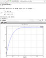 Step response

Now, let's look at the modern, state-space approach. If we have the matrices A, B, C and D, we can plug these into the step function, as shown:
step(A, B, C, D);
or, we can optionally include a vector for time, t:
step(A, B, C, D, t);
Again, if we supply results on the left-hand side of the equation, MATLAB will not automatically produce a plot for us.
If we didn't get an automatic plot, and we want to produce our own, we type:
[y, x, t] = step(NUM, DEN, t);
And then we can create a graph using the plot command:
plot(t, y);
y is the output magnitude of the step response, while x is the internal state of the system from the state-space equations:


Classical ↔ Modern
[edit | edit source]MATLAB contains features that can be used to automatically convert to the state-space representation from the Laplace representation. This function, tf2ss, is used as follows:
[A, B, C, D] = tf2ss(NUM, DEN);
Where NUM and DEN are the coefficient vectors of the numerator and denominator of the transfer function, respectively.
In a similar vein, we can convert from the Laplace domain back to the state-space representation using the ss2tf function, as such:
[NUM, DEN] = ss2tf(A, B, C, D);
Or, if we have more than one input in a vector u, we can write it as follows:
[NUM, DEN] = ss2tf(A, B, C, D, u);
The u parameter must be provided when our system has more than one input, but it does not need to be provided if we have only 1 input. This form of the equation produces a transfer function for each separate input. NUM and DEN become 2-D matricies, with each row being the coefficients for each different input.
z-Domain Digital Filters
[edit | edit source]Let us now consider a digital system with the following generic transfer function in the Z domain:

Where n(z) and d(z) are the numerator and denominator polynomials of the transfer function, respectively. The filter command can be used to apply an input vector x to the filter. The output, y, can be obtained from the following code:
y = filter(n, d, x);
The word "filter" may be a bit of a misnomer in this case, but the fact remains that this is the method to apply an input to a digital system. Once we have the output magnitude vector, we can plot it using our plot command:
plot(y);
To get the step response of the digital system, we must first create a step function using the ones command:
u = ones(1, N);
Where N is the number of samples that we want to take in our digital system (not to be confused with "n", our numerator coefficient). Once we have produced our unit step function, we can pass this function through our digital filter as such:
y = filter(n, d, u);
And we can plot y:
plot(y);
State-Space Digital Filters
[edit | edit source]Likewise, we can analyze a digital system in the state-space representation. If we have the following digital state relationship:
![{\displaystyle x[k+1]=Ax[k]+Bu[k]}](https://wikimedia.org/api/rest_v1/media/math/render/svg/968e943803299b5d109c4f8c3c9f30267d4253a6)
![{\displaystyle y[k]=Cx[k]+Du[k]}](https://wikimedia.org/api/rest_v1/media/math/render/svg/4f519a3e55979d6f94be1a47fcec83f3b7c6d06f)
We can convert automatically to the pulse response using the ss2tf function, that we used above:
[NUM, DEN] = ss2tf(A, B, C, D);
Then, we can filter it with our prepared unit-step sequence vector, u:
y = filter(num, den, u)
this will give us the step response of the digital system in the state-space representation.
Root Locus Plots
[edit | edit source]MATLAB supplies a useful, automatic tool for generating the root-locus graph from a transfer function: the rlocus command. In the transfer function domain, or the state space domain respectively, we have the following uses of the function:
rlocus(num, den);
And:
rlocus(A, B, C, D);
These functions will automatically produce root-locus graphs of the system. However, if we provide left-hand parameters:
[r, K] = rlocus(num, den);
Or:
[r, K] = rlocus(A, B, C, D);
The function won't produce a graph automatically, and you will need to produce one yourself. There is also an optional additional parameter for gain, K, that can be supplied:
rlocus(num, den, K);
Or:
rlocus(A, B, C, D, K);
If K is not supplied, MATLAB will supply an automatic gain value for you.
Once we have our values [r, K], we can plot a root locus:
plot(r);
The rlocus command cannot be used with MIMO systems, so if your system is a MIMO system, you must separate out your coefficient matrices to isolate each separate Input-output pair, and graph each individually.
Here is a sample screenshot:
-
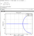 root-locus

Digital Root-Locus
[edit | edit source]Creating a root-locus diagram for a digital system is exactly the same as it is for a continuous system. The only difference is the interpretation of the results, because the stability region for digital systems is different from the stability region for continuous systems. The same rlocus function can be used, in the same manner as is used above.
Bode Plots
[edit | edit source]MATLAB also offers a number of tools for examining the frequency response characteristics of a system, both using Bode plots, and using Nyquist charts. To construct a Bode plot from a transfer function, we use the following command:
[mag, phase, omega] = bode(NUM, DEN, omega);
Or:
[mag, phase, omega] = bode(A, B, C, D, u, omega);
Where "omega" is the frequency vector where the magnitude and phase response points are analyzed. If we want to convert the magnitude data into decibels, we can use the following conversion:
magdb = 20 * log10(mag);
This conversion should be known well enough by now that it doesn't require explanation.
When talking about Bode plots in decibels, it makes the most sense (and is the most common occurrence) to also use a logarithmic frequency scale. To create such a logarithmic sequence in omega, we use the logspace command, as such:
omega = logspace(a, b, n);
This command produces n points, spaced logarithmicly, from up to .


If we use the bode command without left-hand arguments, MATLAB will produce a graph of the bode phase and magnitude plots automatically.
The bode command, if used with a MIMO system, will use subplots to produce all the input-output relationship graphs on a single plot window. for a system with multiple inputs and multiple outputs, this can become difficult to see clearly. In these cases, it is typically better to separate out your coefficient matrices to isolate each individual input-output pair.
Here is a sample screenshot:
-
 Bode plot (Frequency response)

Nyquist Plots
[edit | edit source]In addition to the bode plots, we can create nyquist charts by using the nyquist command. The nyquist command operates in a similar manner to the bode command (and other commands that we have used so far):
[real, imag, omega] = nyquist(NUM, DEN, omega);
Or:
[real, imag, omega] = nyquist(A, B, C, D, u, omega);
Here, "real" and "imag" are vectors that contain the real and imaginary parts of each point of the nyquist diagram. If we don't supply the right-hand arguments, the nyquist command automatically produces a nyquist plot for us.
Like the bode command, the nyquist command will use subplots to display the input-output relations of MIMO systems on a single plot window. If there are multiple input-output pairs, it can be difficult to see the individual graphs.
Here is a sample screenshot:
-
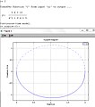 Nyquist plot

Lyapunov Equations
[edit | edit source]Controllability
[edit | edit source]A controllability matrix can be constructed using the ctrb command. The controllability gramian can be constructed using the gram command.
Observability
[edit | edit source]An observability matrix can be constructed using the command obsv
Empirical Gramians
[edit | edit source]Empirical gramians can be computed for linear and also nonlinear control systems. The empirical gramian framework emgr allows the computation of the controllability, observability and cross gramian; it is compatible with MATLAB and OCTAVE and does not require the control systems toolbox.
Further reading
[edit | edit source]- Ogata, Katsuhiko, "Solving Control Engineering Problems with MATLAB", Prentice Hall, New Jersey, 1994. ISBN 0130459070
- MATLAB Programming.
- http://octave.sourceforge.net/
- MATLAB Category on ControlTheoryPro.com
- Empirical Gramian Framework