Control Systems/Feedback Loops
Feedback
[edit | edit source]A feedback loop is a common and powerful tool when designing a control system. Feedback loops take the system output into consideration, which enables the system to adjust its performance to meet a desired output response.
When talking about control systems it is important to keep in mind that engineers typically are given existing systems such as actuators, sensors, motors, and other devices with set parameters, and are asked to adjust the performance of those systems. In many cases, it may not be possible to open the system (the "plant") and adjust it from the inside: modifications need to be made external to the system to force the system response to act as desired. This is performed by adding controllers, compensators, and feedback structures to the system.
Basic Feedback Structure
[edit | edit source]
This is a basic feedback structure. Here, we are using the output value of the system to help us prepare the next output value. In this way, we can create systems that correct errors. Here we see a feedback loop with a value of one. We call this a unity feedback.
Here is a list of some relevant vocabulary, that will be used in the following sections:
- Plant
- The term "Plant" is a carry-over term from chemical engineering to refer to the main system process. The plant is the preexisting system that does not (without the aid of a controller or a compensator) meet the given specifications. Plants are usually given "as is", and are not changeable. In the picture above, the plant is denoted with a P.
- Controller
- A controller, or a "compensator" is an additional system that is added to the plant to control the operation of the plant. The system can have multiple compensators, and they can appear anywhere in the system: Before the pick-off node, after the summer, before or after the plant, and in the feedback loop. In the picture above, our compensator is denoted with a C.
- Summer
- A summer is a symbol on a system diagram, (denoted above with parenthesis) that conceptually adds two or more input signals, and produces a single sum output signal.
- Pick-off node
- A pickoff node is simply a fancy term for a split in a wire.
- Forward Path
- The forward path in the feedback loop is the path after the summer, that travels through the plant and towards the system output.
- Reverse Path
- The reverse path is the path after the pick-off node, that loops back to the beginning of the system. This is also known as the "feedback path".
- Unity feedback
- When the multiplicative value of the feedback path is 1.
Negative vs Positive Feedback
[edit | edit source]It turns out that negative feedback is almost always the most useful type of feedback. When we subtract the value of the output from the value of the input (our desired value), we get a value called the error signal. The error signal shows us how far off our output is from our desired input.
Positive feedback has the property that signals tend to reinforce themselves, and grow larger. In a positive feedback system, noise from the system is added back to the input, and that in turn produces more noise. As an example of a positive feedback system, consider an audio amplification system with a speaker and a microphone. Placing the microphone near the speaker creates a positive feedback loop, and the result is a sound that grows louder and louder. Because the majority of noise in an electrical system is high-frequency, the sound output of the system becomes high-pitched.
Example: State-Space Equation
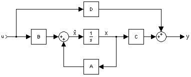
[edit | edit source]In the previous chapter, we showed you this picture:

Now, we will derive the I/O relationship into the state-space equations. If we examine the inner-most feedback loop, we can see that the forward path has an integrator system, , and the feedback loop has the matrix value A. If we take the transfer function only of this loop, we get:
Pre-multiplying by the factor B, and post-multiplying by C, we get the transfer function of the entire lower-half of the loop:
We can see that the upper path (D) and the lower-path Tlower are added together to produce the final result:
Now, for an alternate method, we can assume that x' is the value of the inner-feedback loop, right before the integrator. This makes sense, since the integral of x' should be x (which we see from the diagram that it is. Solving for x', with an input of u, we get:
This is because the value coming from the feedback branch is equal to the value x times the feedback loop matrix A, and the value coming from the left of the summer is the input u times the matrix B.
If we keep things in terms of x and u, we can see that the system output is the sum of u times the feed-forward value D, and the value of x times the value C:
These last two equations are precisely the state-space equations of our system.
Feedback Loop Transfer Function
[edit | edit source]We can solve for the output of the system by using a series of equations:
and when we solve for Y(s) we get:
[Feedback Transfer Function]
The reader is encouraged to use the above equations to derive the result by themselves.
The function E(s) is known as the error signal. The error signal is the difference between the system output (Y(s)), and the system input (X(s)). Notice that the error signal is now the direct input to the system G(s). X(s) is now called the reference input. The purpose of the negative feedback loop is to make the system output equal to the system input, by identifying large differences between X(s) and Y(s) and correcting for them.
Example: Elevator
[edit | edit source]Here is a simple example of reference inputs and feedback systems:
There is an elevator in a certain building with 5 floors. Pressing button "1" will take you to the first floor, and pressing button "5" will take you to the fifth floor, etc. For reasons of simplicity, only one button can be pressed at a time.
Pressing a particular button is the reference input of the system. Pressing "1" gives the system a reference input of 1, pressing "2" gives the system a reference input of 2, etc. The elevator system then, tries to make the output (the physical floor location of the elevator) match the reference input (the button pressed in the elevator). The error signal, e(t), represents the difference between the reference input x(t), and the physical location of the elevator at time t, y(t).
Let's say that the elevator is on the first floor, and the button "5" is pressed at time t0. The reference input then becomes a step function:
Where we are measuring in units of "floors". At time t0, the error signal is:
Which means that the elevator needs to travel upwards 4 more floors. At time t1, when the elevator is at the second floor, the error signal is:
Which means the elevator has 3 more floors to go. Finally, at time t4, when the elevator reaches the top, the error signal is:
And when the error signal is zero, the elevator stops moving. In essence, we can define three cases:
- e(t) is positive: In this case, the elevator goes up one floor, and checks again.
- e(t) is zero: The elevator stops.
- e(t) is negative: The elevator goes down one floor, and checks again.
State-Space Feedback Loops
[edit | edit source]In the state-space representation, the plant is typically defined by the state-space equations:
The plant is considered to be pre-existing, and the matrices A, B, C, and D are considered to be internal to the plant (and therefore unchangeable). Also, in a typical system, the state variables are either fictional (in the sense of dummy-variables), or are not measurable. For these reasons, we need to add external components, such as a gain element, or a feedback element to the plant to enhance performance.
Consider the addition of a gain matrix K installed at the input of the plant, and a negative feedback element F that is multiplied by the system output y, and is added to the input signal of the plant. There are two cases:
- The feedback element F is subtracted from the input before multiplication of the K gain matrix.
- The feedback element F is subtracted from the input after multiplication of the K gain matrix.
In case 1, the feedback element F is added to the input before the multiplicative gain is applied to the input. If v is the input to the entire system, then we can define u as:
In case 2, the feeback element F is subtracted from the input after the multiplicative gain is applied to the input. If v is the input to the entire system, then we can define u as:
Open Loop vs Closed Loop
[edit | edit source]
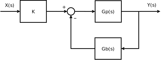
Let's say that we have the generalized system shown above. The top part, Gp(s) represents all the systems and all the controllers on the forward path. The bottom part, Gb(s) represents all the feedback processing elements of the system. The letter "K" in the beginning of the system is called the Gain. We will talk about the gain more in later chapters. We can define the Closed-Loop Transfer Function as follows:
[Closed-Loop Transfer Function]
If we "open" the loop, and break the feedback node, we can define the Open-Loop Transfer Function, as:
[Open-Loop Transfer Function]
We can redefine the closed-loop transfer function in terms of this open-loop transfer function:
These results are important, and they will be used without further explanation or derivation throughout the rest of the book.
Placement of a Controller
[edit | edit source]There are a number of different places where we could place an additional controller.
Each location has certain benefits and problems, and hopefully we will get a chance to talk about all of them.
Second-Order Systems
[edit | edit source]The general expression of the transfer function of a second order system is given as:
where and are damping ratio and natural frequency of the system respectively.
Damping Ratio
[edit | edit source]The damping ratio is defined by way of the sign . The damping ratio gives us an idea about the nature of the transient response detailing the amount of overshoot & oscillation that the system will undergo. This is completely regardless of time scaling.
If :
- = zero, the system is undamped;
- < 1, the system is underdamped;
- = 1, the system is critically damped;
- > 1, the system is overdamped.
is used in conjunction with the natural frequency to determine system properties. To find the zeta value you must first find the natural response!
Natural Frequency
[edit | edit source]Natural Frequency, denoted by is defined as the frequency with which the system would oscillate if it were not damped and we define the damping ratio as .


