
Fractals/Iterations in the complex plane/Julia set
"... a single algorithm for computing all quadratic Julia sets does not exist."[1]
This book shows how to code different algorithms for drawing sets in dynamical plane : Julia, Filled-in Julia or Fatou sets for complex quadratic polynomial.
It is divided in 2 parts :
- description of various algorithms[2]
- descriptions of technics for visualisation of various sets in dynamic plane
- Julia set
- Fatou set
- basin of attraction of infinity ( open set)
- basin of attraction of finite attractor

Algorithms
[edit | edit source]Methods based on speed of attraction
[edit | edit source]Here color is proportional to speed of attraction ( convergence to attractor). These methods are used in Fatou set.
How to find:
Basin of attraction to infinity = exterior of filled-in Julia set and The Divergence Scheme = Escape Time Method ( ETM )
[edit | edit source]First read definitions
Here one computes forward iterations of a complex point Z0:

Here is function which computes the last iteration, that is the first iteration that lands in the target set ( for example leaves a circle around the origin with a given escape radius ER ) for the iteration of the complex quadratic polynomial above. It is a iteration ( integer) for which (abs(Z)>ER). It can also be improved [5]
C version ( here ER2=ER*ER) using double floating point numbers ( without complex type numbers) :
 int GiveLastIteration(double Zx, double Zy, double Cx, double Cy, int IterationMax, int ER2)
 {
  double Zx2, Zy2; /* Zx2=Zx*Zx;  Zy2=Zy*Zy  */
  int i=0;
  Zx2=Zx*Zx;
  Zy2=Zy*Zy;
  while (i<IterationMax && (Zx2+Zy2<ER2) ) /* ER2=ER*ER */
  {
   Zy=2*Zx*Zy + Cy;
   Zx=Zx2-Zy2 +Cx;
   Zx2=Zx*Zx;
   Zy2=Zy*Zy;
   i+=1;
  }
  return i;
 }
C with complex type from GSL :[6]
#include <gsl/gsl_complex.h>
#include <gsl/gsl_complex_math.h>
#include <stdio.h>
// gcc -L/usr/lib -lgsl -lgslcblas -lm t.c
// function fc(z) = z*z+c

gsl_complex f(gsl_complex z, gsl_complex c) {
  return gsl_complex_add(c, gsl_complex_mul(z,z));
}

int main () {
  gsl_complex c = gsl_complex_rect(0.123, 0.125);
  gsl_complex z = gsl_complex_rect(0.0, 0.0);
  int i;
  for (i = 0; i < 10; i++) {
    z = f(z, c);
    double zx = GSL_REAL(z);
    double zy = GSL_IMAG(z);
    printf("Real: %f4 Imag: %f4\n", zx, zy);
  }
  return 0;
}
C++ versions:
 int GiveLastIteration(complex C,complex Z , int imax, int ER)
  {
   int i; // iteration number
   for(i=0;i<=imax-1;i++) // forward iteration
    {
      Z=Z*Z+C; // overloading of operators
      if(abs(Z)>ER) break;
    }
   return i;
 }
#include <complex> // C++ complex library

// bailout2 = bailout * bailout
// this function is based on function esctime from mndlbrot.cpp
// from program mandel ver. 5.3 by Wolf Jung
// http://www.mndynamics.com/indexp.html

int escape_time(complex<double> Z, complex<double> C , int iter_max,  double bailout2)
{
  // z= x+ y*i   z0=0
  long double x =Z.real(), y =Z.imag(),  u ,  v ;
  int iter; // iteration
  for ( iter = 0; iter <= iter_max-1; iter++)
  { u = x*x;
    v = y*y;
    if ( u + v <= bailout2 )
       {
         y = 2 * x * y + C.imag();
         x = u - v + C.real();
       } // if
    else break;
  } // for
  return iter;
} // escape_time
Delphi version ( using user defined complex type, cabs and f functions )
function GiveLastIteration(z,c:Complex;ER:real;iMax:integer):integer;
  var i:integer;
  begin
  i:=0;
  while (cabs(z)<ER) and (i<iMax) do
    begin
      z:= f(z,c);
      inc(i);
    end;
  result := i;
end;
where :
type complex = record x, y: real; end;

function cabs(z:complex):real;
begin
  cabs:=sqrt(z.x*z.x+z.y*z.y)
end;

function f(z,c:complex):complex; // complex quadratic polynomial
  var tmp:complex;
begin
  tmp.x := (z.x*z.x) - (z.y*z.y) + c.x;
  tmp.y := 2*z.x*z.y + c.y ;
  result := tmp;

end;
Delphi version without explicit definition of complex numbers :
function GiveLastIteration(zx0,zy0,cx,cy,ER2:extended;iMax:integer):integer;
  // iteration of z=zx+zy*i under fc(z)=z*z+c
  // where c=cx+cy*i
  // until abs(z)<ER  ( ER2=ER*ER )  or i>=iMax
  var i:integer;
      zx,zy,
      zx2,zy2:extended;
  begin
  zx:=zx0;
  zy:=zy0;
  zx2:=zx*zx;
  zy2:=zy*zy;

  i:=0;
  while (zx2+zy2<ER2) and (i<iMax) do
    begin
      zy:=2*zx*zy + cy;
      zx:=zx2-zy2 +cx;
      zx2:=zx*zx;
      zy2:=zy*zy;
      //
      inc(i);
    end;
  result := i;
end;
Euler version by R. Grothmann ( with small change : from z^2-c to z^2+c) [8]
function iter (z,c,n=100) ...

h=z;
loop 1 to n;
h=h^2 + c;
if totalmax(abs(h))>1e20; m=#; break; endif;
end;
return {h,m};
endfunction
Lisp version
This version uses complex numbers. It makes the code short but is also inefficient.
((DEFUN GIVELASTITERATION (Z_0 _C IMAX ESCAPE_RADIUS)
  (SETQ Z Z_0)
  (SETQ I 0)
  (LOOP WHILE (AND (< I IMAX) (< (ABS Z) ESCAPE_RADIUS)) DO
    (INCF I)
    (SETQ Z (+ (* Z Z) _C)))
   I)
Maxima version :
/* easy to read but very slow version, uses complex type numbers */
GiveLastIteration(z,c):=
 block([i:0],
  while abs(z)<ER and i<iMax
     do (z:z*z + c,i:i+1),
  i)$
/* faster version, without use of complex type numbers,
   compare with c version, ER2=ER*ER */
GiveLastIter(zx,zy,cx,cy,ER2,iMax):=
block(
 [i:0,zx2,zy2],
 zx2:zx*zx,
 zy2:zy*zy,
 while (zx2+zy2<ER2) and i<iMax do
 (
  zy:2*zx*zy + cy,
  zx:zx2-zy2 +cx,
  zx2:zx*zx,
  zy2:zy*zy,
  i:i+1
 ),
 return(i)
);
Boolean Escape time
[edit | edit source]Algorithm: for every point z of dynamical plane (z-plane) compute iteration number ( last iteration) for which magnitude of z is greater than escape radius. If last_iteration=max_iteration then point is in filled-in Julia set, else it is in its complement (attractive basin of infinity ). Here one has 2 options, so it is named boolean algorithm.
if (LastIteration==IterationMax)
   then color=BLACK;   /* bounded orbits = Filled-in Julia set */
   else color=WHITE;  /* unbounded orbits = exterior of Filled-in Julia set  */
In theory this method is for drawing Filled-in Julia set and its complement ( exterior), but when c is Misiurewicz point ( Filled-in Julia set has no interior) this method draws nothing. For example for c=i . It means that it is good for drawing interior of Filled-in Julia set.
ASCII graphic
[edit | edit source]; common lisp
(loop for y from -2 to 2 by 0.05 do
(loop for x from -2 to 2 by 0.025 do
(let* ((z (complex x y))
(c (complex -1 0))
(iMax 20)
(i 0))
(loop while (< i iMax ) do
(setq z (+ (* z z) c))
(incf i)
(when (> (abs z) 2) (return i)))
(if (= i iMax) (princ (code-char 42)) (princ (code-char 32)))))
(format t "~%"))
PPM file with raster graphic
[edit | edit source]
Integer escape time = Level Sets of the Basin of Attraction of Infinity = Level Sets Method= LSM/J
[edit | edit source]-
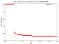 level sets of escape time for C=0 and 0.9<Z<1.5
 -


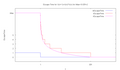
Escape time measures time of escaping to infinity ( infinity is superattracting point for polynomials). Time is measured in steps ( iterations = i) needed to escape from circle of given radius ( ER= Escape Radius).
One can see few things:
- this is discontinuous function
- i is iMax for z in Filled-in Julia set
- i=0 for x0>ER
- this is nonlinear function
Level sets here are sets of points with the same escape time. Here is algorithm of choosing color in black & white version.
  if (LastIteration==IterationMax)
   then color=BLACK;   /* bounded orbits = Filled-in Julia set */
   else   /* unbounded orbits = exterior of Filled-in Julia set  */
        if ((LastIteration%2)==0) /* odd number */
           then color=BLACK;
           else color=WHITE;
Here is the c function which:
- uses complex double type numbers
- computes 8 bit color ( shades of gray)
- checks both escape and attraction test
unsigned char ComputeColorOfLSM(complex double z){

 int nMax = 255;
  double cabsz;
  unsigned char iColor;

  int n;

  for (n=0; n < nMax; n++){ //forward iteration
	cabsz = cabs(z);
    	if (cabsz > ER) break; // esacping
    	if (cabsz< PixelWidth) break; // fails into finite attractor = interior


     	z = z*z +c ; /* forward iteration : complex quadratic polynomial */
  }


  iColor = 255 - 255.0 * ((double) n)/20; // nMax or lower walues in denominator


  return iColor;
}
"if a 2-variable function z = f(x,y) has non-extremal critical points, i.e. it has saddle points, then it's best if the contour z heights are chosen so that the saddle points are on a contour, so that the crossing contours appear visually."Alan Ableson
How to choose parameters for which Level curves cross critical point ( and it's preimages ) ?
- choose the parameter c such that it is on an escape line, then the critical value will be on an escape line as well
- choose escape radius equal to n=th iteration of critical value
// find such ER for LSM/J that level curves croses critical point and it's preimages ( only for disconnected Julia sets)
double GiveER(int i_Max){

	complex double z= 0.0; // criical point
	int i;
	 ; // critical point escapes very fast here. Higher valus gives infinity
	for (i=0; i< i_Max; ++i ){
		z=z*z +c;

	 }

	 return cabs(z);


}
- level curves cross at critical point
-
 not cross
 -
 cross
cross -
 cross
cross
.jpg)


Normalized iteration count (real escape time or fractional iteration or Smooth Iteration Count Algorithm (SICA))
[edit | edit source]-
 integer escape time = LSM
 -
 real escape time
 -
 Escape time for C=0 and 0.5<Z<2.5


Math formula :

Maxima version :
GiveNormalizedIteration(z,c,E_R,i_Max):=
/* */
block(
 [i:0,r],
 while abs(z)<E_R and i<i_Max
   do (z:z*z + c,i:i+1),
 r:i-log2(log2(cabs(z))),
 return(float(r))
)$
In Maxima log(x) is a natural (base e) logarithm of x. To compute log2 use :
log2(x) := log(x) / log(2);
description:
- FF : julia-smooth-colouring-how-to-do
- stefan bion : fraktal-generator/colormapping/
- FF smooth-histogram-rendering/
- FF creating-a-good-palette-using-bezier-interpolation/
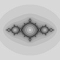
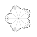
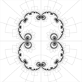
Level Curves of escape time Method = eLCM/J
[edit | edit source]-
 edge detection Image and C code
 -
 preimages of circle


These curves are boundaries of Level Sets of escape time ( eLSM/J ). They can be drawn using these methods:
- edge detection of Level Curves ( =boundaries of Level sets).
- Algorithm based on paper by M. Romera et al.[9]
- Sobel filter
- drawing lemniscates = curves , see explanation and source code
- drawing circle and its preimages. See this image, explanation and source code
- method described by Harold V. McIntosh[10]


/* Maxima code : draws lemniscates of Julia set */
c: 1*%i;
ER:2;
z:x+y*%i;
f[n](z) := if n=0 then z else (f[n-1](z)^2 + c);
load(implicit_plot); /* package by Andrej Vodopivec */
ip_grid:[100,100];
ip_grid_in:[15,15];
implicit_plot(makelist(abs(ev(f[n](z)))=ER,n,1,4),[x,-2.5,2.5],[y,-2.5,2.5]);
Density of level curves[11]
"The spacing between level curves is a good way to estimate gradients: level curves that are close together represent areas of steeper descent/ascent." [12]
"The density of the contour lines tells how steep is the slope of the terrain/function variation. When very close together it means f is varying rapidly (the elevation increase or decrease rapidly). When the curves are far from each other the variation is slower" [13]
How to control level curves
- escape radius
- shape of target set
- manually
- drawing equipotential lines
- changing level sets ( level curves are boundaries of level sets)
Basin of attraction of finite attractor = interior of filled-in Julia set
[edit | edit source]- How to find periodic attractor ?
- How many iterations is needed to reach attractor ?

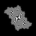
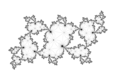
Components of Interior of Filled Julia set ( Fatou set)
[edit | edit source]- use limited color ( palette = list of numbered colors)
- find period of attracting cycle
- find one point of attracting cycle
- compute number of iteration after when point reaches the attractor
- color of component=iteration % period[14]
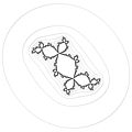
- use edge detection for drawing Julia set
-
 Components of Fatou set for period 4
 -
 Components of Fatou set for period 3
 -
 In case of Siegel disc critical orbit is a boundary Siegel disc compponent. All other componnats are preimages of this component


Internal Level Sets
[edit | edit source]See :
- algorithm 0 of program Mandel by Wolf Jung
-
 attracting
 -
 attracting
 -
 attracting
 -
 parabolic
 -
Video for c along internal ray 0
-
 weakly attracting
 -

-

-

-
 parabolic period 3


%3D_z%5E3%2B(1.0149042485835864102%2B0.10183008497976470119i)*z;_(zoom).png)

%3D1_over_az5%2Bz3%2Bbz.png)
%3D1_over_z3%2Bz*(-3-3*I).png)
_%3D_rho_*_z%5E2_*_(z-3)_over_(1-3z)_with_LCM_and_critical_orbit.png)
How to choose size of attracting trap such that level curves cross at critical point ?
It depends on
- dynamic type ( superattracting/attracting, parabolic, repelling)
- period ( child period in the parabolic case)
- petal in the parabolic case :
- for period 1 and 2 : radius of a circle with parabolic point on it's boundary
- for higher periods sector of the circle with center at parabolic point
- for other cases ( except repelling) it is radius of the circle with attractor as a center
int local_setup(double cx){

	c = cx;
	zp = GiveFixed(c);

	switch ( DynamicType){
		case repelling: // no  interior = no attracting fixed point = only escaping points

			break;
		case attracting:
			delta = sqrt(1.0 - 4.0* creal(c));  // delta is a distance between alfa and beta fixed points
			AR =  delta /20.0;

	  		break;

		case superattracting: // cabs(zp - zcr_last ) < PixelWidth
			AR = 30.0* PixelWidth * iWidth / 5000 ; //
	  		break;

		case parabolic:
				// zcr_last < parabolic_trap_center < zp
				int i; /* nr of point of critical orbit */
  				complex double z = zcr;
  				for (i=1;i<IterMax ; ++i)
    					{ z = f(z); }
  				zcr_last = z;
				//
				AR = (zp - zcr_last)/2.0;
				parabolic_trap_center = ( creal(zp) + creal(zcr_last))/ 2.0;
				break;
		default:
	}


	AR2 = AR*AR;


	return 0;
}

// and print program info
fprintf (stdout, "DynamicType value is setup manually; Once can do it also numerically ( from multiplier of fixed point alfa or from some other properities)\n");
  		switch ( DynamicType){
		case repelling:
				fprintf (stdout, "\tThere is only one Fatou basin: basin of infinity \n");
				fprintf (stdout, "\tthere is no interior = Julia set is disconnected \n");
				fprintf (stdout, "\tcritical point z=0 is repelling = attracted to infinity \n");
				break;
		case attracting:
	  			fprintf (stdout, "\tbasin type is attracting \n");
	  			fprintf (stdout, "\tzcr_last =  %.16f \talfa fixed point zp = %.16f\n", creal (zcr_last), creal(zp));//
	  			fprintf (stdout, "\tdelta =  %.16f is the distance between fixed points\n", delta);//
	  			fprintf (stdout, "\tAtracting Radius AR is set manually  = %.16f = %f * PixelWidth = %f * ImageWidth \n", AR, AR / PixelWidth, AR /ImageWidth );
	  			break;

		case superattracting:
				fprintf (stdout, "\tbasin type is superattracting \n");
	  			fprintf (stdout, "\tzcr =  %.16f  = zp = %.16f\n", creal (zcr), creal(zp));//
	  			fprintf (stdout, "\tAtracting Radius AR is set manually  = %.16f = %f *PixelWidth = %f *ImageWidth \n", AR, AR / PixelWidth, AR /ImageWidth);
	  			break;

		case parabolic:
				fprintf (stdout, "\tbasin type  is parabolic \n");
				fprintf (stdout, "\tzcr_last =  %.16f < parabolic_trap_center = %.16f < zp = %.16f\n", creal (zcr_last), creal (parabolic_trap_center), creal(zp));//
				fprintf (stdout, "\tzp - zcr_last =  %.16f AR*2 = %.16f \t difference = %.16f\n", creal (zp - zcr_last), AR *2.0, creal (zp - zcr_last) -  AR *2.0);//
				fprintf (stdout, "\tAtracting Radius AR is tuned  = (zp - zcr_last)/2 = %.16f = %f *PixelWidth = %f *ImageWidth \n", AR, AR / PixelWidth, AR /ImageWidth);
				fprintf (stdout, "\tparabolic_trap_center z =  %.16f %+.16f*i  \n", creal (parabolic_trap_center), cimag (parabolic_trap_center));// parabolic_trap_center
				break;
		default:


	}
Steps for parabolic basin
- choose component with critical point inside
- choose trap
Trap is a disk
- inside component with critical point inside
- trap has parabolic point on it's boundary
- center of the trap is the midpoint between last point of critical orbit and fixed point
- radius of the trap is half of distance between fixed point and last point of critical orbit
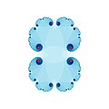
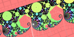
Decomposition of target set
[edit | edit source]- Decomposition
-
 Binary decomposition of whole dynamical plane with circle Julia set c = 0
 -
Binary decomposition along internal ray 0
-
 from decomposition to parabolic checkerboard
 -
 boundaries of BD in the exterior and interior of Mandelbrot set


Examples
Binary decomposition
[edit | edit source]-
 LC of BDM
 -

-
 1
1 -
 2
2 -
 3
3 -
 4
4 -
 11
11

_%3D_z%5E2_%2B_i_using_BDM_DEM_LSM.png)


_%3D_z*z_%2B_0.25%2B0.5i_BDM.png)
_%3D_z*z_-0.6978381951224250%2B0.2793041341013660i.png)
Here color of pixel ( exterior of Julia set) is proportional to sign of imaginary part of last iteration ( cimag) = the radial borders of are at dyadic angles (shows external rays at dyadic angles).
Main loop is the same as in escape time.
Radius
- Escape radius ( ER) should be bigger: ER = 200
- attracting radius (AR)
- for superattracting case small: AR = PixelWidth
In other words target set is decompositioned in 2 parts ( binary decomposition) :


Algorithm in pseudocode ( Im(Zn) = Zy ) :
if (LastIteration==IterationMax)
   then color=BLACK;   /* bounded orbits = Filled-in Julia set */
   else   /* unbounded orbits = exterior of Filled-in Julia set  */
        if (Zy>0) /* Zy=Im(Z) */
           then color=BLACK;
           else color=WHITE;
Description
- Mandelbrot Set Glossary and Encyclopedia, by Robert Munafo, (c) 1987-2022.
- mandelbook by Claude Heiland-Allen
unsigned char ComputeColorOfBD (complex double z)
{

  double cabsz;


  int i;			// number of iteration
  for (i = 0; i < IterMax_LSM; ++i)
    {


	cabsz = cabs(z); // numerical speed up : cabs(zp-z) = cabs(z) because zp = zcr = 0

      //
       if ( cabsz > ER  ||  cabsz < AR ) // if z is inside target set ( orbit trap)
       		{
       			if (cimag(z) > 0) // binary decomposition of target set
       				{  return 0;}
       				else {return 255; }


      		}


      z = f(z);

    }

  return iColorOfUnknown;


}
- only boundaries of parabolic BDM for one component Julia sets ( upper row is Blascheke product, lower row is Multibrot set
-
 d=2
d=2 -
 d=3
d=3 -
 d=4
d=4 -
 d=5
d=5 -

-

-

-
_%3D_(z%5Ed_%2B_a)_over_(1_%2B_a*z%5Ed)_with_a_%3D_(d_-_1)_over_(_d_%2B_1)_for_d_%3D_2.png)
_%3D_(z%5Ed_%2B_a)_over_(1_%2B_a*z%5Ed)_with_a_%3D_(d_-_1)_over_(_d_%2B_1)_for_d_%3D_3.png)
_%3D_(z%5Ed_%2B_a)_over_(1_%2B_a*z%5Ed)_with_a_%3D_(d_-_1)_over_(_d_%2B_1)_for_d_%3D_4.png)
_%3D_(z%5Ed_%2B_a)_over_(1_%2B_a*z%5Ed)_with_a_%3D_(d_-_1)_over_(_d_%2B_1)_for_d_%3D_5.png)
_%3D_z*z_%2B_0.25.png)
_%3D_z%5E3_%2B_0.3849001794597505.png)
_%3D_z*z*z*z_%2B_0.472464424146544.png)
_%3D_z*z*z*z*z_%2B_0.5349922439811376.png)
- evolution of dynamics along internal/external ray 0
-
center = superattracting
-
 attracting
 -
 parabolic
 -
 repelling


Attracting case is used for "field lines" coloring method by Gertbuschmann


These curves :
- are boundaries of binare decomposition boxes
- are not field lines of potential = external rays
Notes
- if the escape radius is too low, then binary (or ternary, etc) decomposition rays will have visible discontinuities at iteration bands. increasing escape radius makes discontinuities smaller, but changes the aspect ratio
- mrob says exp(pi) is the best escape radius for binary decomposition as it makes boxes have square aspect ratio (possibly more visible when using exponential map transformation?)
rotation of target set by internal angle
[edit | edit source]-
modified binary decomposition
-


 // for MBD
 double t0 = 1.0 / 3.0; // period = 3

// Modified BD
unsigned char ComputeColorOfMBD (complex double z)
{

  double cabsz;
  double turn;

  int i;			// number of iteration
  for (i = 0; i < IterMax_LSM; ++i)
    {


	cabsz = cabs(z); // numerical speed up : cabs2(zp-z) = cabs2(z) because zp = zcr = 0

      //  if z is inside target set ( orbit trap) = exterior of circle with radius ER
       if ( cabsz > ER  ) // exterior
       		{
       			if (creal(z) > 0) // binary decomposition of target set
       				{  return 0;}
       				else {return 255; }


      		}

      	if ( cabsz  < AR ) // if z is inside target set ( orbit trap) = interior of circle with radius AR
      		{
      			turn = c_turn(z);
      			if (turn < t0 || turn > t0+0.5) // modified binary decomposition of target set
      				{  return 0;}
       				else {return 255; }


      		}


      z = f(z);

    }

  return iColorOfUnknown;


}
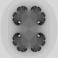
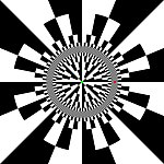
Constant number of iterations
[edit | edit source]- Modified Decomposition
-
 Modified binary decomposition of whole dynamical plane with circle Julia set. Image with src code
 -
 Another modification of binary decomposition
 -
 Modified decomposition of dynamical plane with dendrite Julia set. Image with src code
 -
 Modified decomposition of dynamical plane with basilica Julia set. Image with src code
 -

-


Here exterior of Julia set is decompositioned into radial level sets.
It is because main loop is without bailout test and number of iterations ( iteration max) is constant.
It creates radial level sets.
See also:
- mandel : algorithm 9 = zeros of qn(c)
- video by bryceguy72[15]
- video by FreymanArt[16]
  for (Iteration=0;Iteration<8;Iteration++)
 /* modified loop without checking of abs(zn) and low iteration max */
    {
    Zy=2*Zx*Zy + Cy;
    Zx=Zx2-Zy2 +Cx;
    Zx2=Zx*Zx;
    Zy2=Zy*Zy;
   };
  iTemp=((iYmax-iY-1)*iXmax+iX)*3;
  /* --------------- compute  pixel color (24 bit = 3 bajts) */
 /* exterior of Filled-in Julia set  */
 /* binary decomposition  */
  if (Zy>0 )
   {
    array[iTemp]=255; /* Red*/
    array[iTemp+1]=255;  /* Green */
    array[iTemp+2]=255;/* Blue */
  }
  if (Zy<0 )
   {
    array[iTemp]=0; /* Red*/
    array[iTemp+1]=0;  /* Green */
    array[iTemp+2]=0;/* Blue */
  };
It is also related with automorphic function for the group of Mobius transformations [17]
BDM in the attracting domain
[edit | edit source]BDM in the attracting domain ( usually interior of Julia sets ) gives (pseudo) Field lines
Explanation by Gert Buschmann


In each Fatou domain (that is not neutral) there are two systems of lines orthogonal to each other: the equipotential lines (for the potential function or the real iteration number) and the field lines.
If we colour the Fatou domain according to the iteration number (and not the real iteration number , as defined in the previous section), the bands of iteration show the course of the equipotential lines. If the iteration is towards ∞ (as is the case with the outer Fatou domain for the usual iteration ), we can easily show the course of the field lines, namely by altering the colour according as the last point in the sequence of iteration is above or below the x-axis (first picture), but in this case (more precisely: when the Fatou domain is super-attracting) we cannot draw the field lines coherently - at least not by the method we describe here. In this case a field line is also called an external ray.


Let z be a point in the attracting Fatou domain. If we iterate z a large number of times, the terminus of the sequence of iteration is a finite cycle C, and the Fatou domain is (by definition) the set of points whose sequence of iteration converges towards C. The field lines issue from the points of C and from the (infinite number of) points that iterate into a point of C. And they end on the Julia set in points that are non-chaotic (that is, generating a finite cycle). Let r be the order of the cycle C (its number of points) and let z* be a point in C. We have (the r-fold composition), and we define the complex number α by


If the points of C are , α is the product of the r numbers . The real number 1/|α| is the attraction of the cycle, and our assumption that the cycle is neither neutral nor super-attracting, means that 1 < 1/|α| < ∞. The point z* is a fixed point for , and near this point the map has (in connection with field lines) character of a rotation with the argument β of α (that is, ).


In order to colour the Fatou domain, we have chosen a small number ε and set the sequences of iteration to stop when , and we colour the point z according to the number k (or the real iteration number, if we prefer a smooth colouring). If we choose a direction from z* given by an angle θ, the field line issuing from z* in this direction consists of the points z such that the argument ψ of the number satisfies the condition that


For if we pass an iteration band in the direction of the field lines (and away from the cycle), the iteration number k is increased by 1 and the number ψ is increased by β, therefore the number is constant along the field line.


A colouring of the field lines of the Fatou domain means that we colour the spaces between pairs of field lines: we choose a number of regularly situated directions issuing from z*, and in each of these directions we choose two directions around this direction. As it can happen that the two field lines of a pair do not end in the same point of the Julia set, our coloured field lines can ramify (endlessly) in their way towards the Julia set. We can colour on the basis of the distance to the center line of the field line, and we can mix this colouring with the usual colouring. Such pictures can be very decorative (second picture).
A coloured field line (the domain between two field lines) is divided up by the iteration bands, and such a part can be put into a one-to-one correspondence with the unit square: the one coordinate is (calculated from) the distance from one of the bounding field lines, the other is (calculated from) the distance from the inner of the bounding iteration bands (this number is the non-integral part of the real iteration number). Therefore, we can put pictures into the field lines (third picture).
ToDo
[edit | edit source]- add slope to white
Inverse iteration of repellor for drawing Julia set
Complex potential - Boettcher coordinate
[edit | edit source]DEM/J
[edit | edit source]This algorithm has 2 versions:
Compare it with version for parameter plane and Mandelbrot set : DEM/M It's the same as M-set exterior distance estimation but with derivative w.r.t. Z instead of w.r.t. C.
Convergence
[edit | edit source]In this algorithm distances between 2 points of the same orbit are checked
average discrete velocity of orbit
[edit | edit source]
It is used in case of :
Cauchy Convergence Algorithm (CCA)
[edit | edit source]This algorithm is described by User:Georg-Johann. Here is also Matemathics code by Paul Nylander
Normality
[edit | edit source]Normality In this algorithm distances between points of 2 orbits are checked
Checking equicontinuity by Michael Becker
[edit | edit source]"Iteration is equicontinuous on the Fatou set and not on the Julia set". (Wolf Jung) [18][19]
Michael Becker compares the distance of two close points under iteration on Riemann sphere.[20][21]
This method can be used to draw not only Julia sets for polynomials ( where infinity is always superattracting fixed point) but it can be also applied to other functions ( maps), for which infinity is not an attracting fixed point.[22]
using Marty's criterion by Wolf Jung
[edit | edit source]Wolf Jung is using "an alternative method of checking normality, which is based on Marty's criterion: |f'| / (1 + |f|^2) must be bounded for all iterates." It is implemented in mndlbrot::marty function ( see src code of program Mandel ver 5.3 ). It uses one point of dynamic plane.
Koenigs coordinate
[edit | edit source]Koenigs coordinate are used in the basin of attraction of finite attracting (not superattracting) point (cycle).
Optimisation
[edit | edit source]Distance
[edit | edit source]You don't need a square root to compare distances.[23]
Symmetry
[edit | edit source]Julia sets can have many symmetries [24][25]
Quadratic Julia set has allways rotational symmetry ( 180 degrees) :
colour(x,y) = colour(-x,-y)
when c is on real axis ( cy = 0) Julia set is also reflection symmetric :[26]
colour(x,y) = colour(x,-y)
Algorithm :
- compute half image
- rotate and add the other half
- write image to file [27]
Color
[edit | edit source]- color in computer graphic
- Visualising Julia sets by Georg-Johann
- Combined Methods of Depicting Julia Sets and Parameter Planes by Chris King
- On Fractal Coloring Techniques by Jussi Harkonen Master's Thesis, Department of Mathematics, Åbo Akademi University, Turku, 2007, 61 pages. The thesis was carried out under the supervision of Professor Goran Hognas
- Technical Info - Colorizing by Michael Condron
- Technicolor Julias by Shawn Hargreaves
Sets
[edit | edit source]Target set
[edit | edit source]- trap for forward orbit
- it is a set which captures any orbit tending to fixed / periodic point.
Julia sets
[edit | edit source]"Most programs for computing Julia sets work well when the underlying dynamics is hyperbolic but experience an exponential slowdown in the parabolic case." ( Mark Braverman )[28]
- when Julia set is a set of points that do not escape to infinity under iteration of the quadratic map ( = filled Julia set has no interior = dendrt)
- IIM/J
- DEM/J
- checking normality
- when Julia set is a boundary between 2 basin of attraction ( = filled Julia set has no empty interior) :
- boundary scanning [29]
- edge detection
Fatou set
[edit | edit source]Interior of filled Julia set can be coloured :
- speed of attraction ( integer value = the number of iterations used to guess if a point is in the set ) which is converted to colour ( or shade of gray ) [30]
- Internal Level Sets
- attracting time ( sth like escape time but checks if (abs(z-attractor)<Attracting_radius
- Binary decomposition
- Tessellation of the Interior of Filled Julia Sets by Tomoki KAWAHIRA [31]
- discrete velocity in Siegel disc case
Periodic points
[edit | edit source]More is here
Video
[edit | edit source]One can make videos using :
- zoom into dynamic plane
- changing parametr c along path inside parameter plane[32]
- changing coloring scheme ( for example color cycling )
Examples :
- Target set for internal ray 0 video
- Quadratic Julia set with Internal level sets for internal ray 0 video
More tutorials and code
[edit | edit source]- hypercomplex iterations - book
- hvidtfeldts : distance-estimated-3d-fractals-v-the-mandelbulb-different-de-approximations/
- in Java see Evgeny Demidov
- in C see :
- in C++ see Wolf Jung page,
- in Gnuplot see Tutorial by T.Kawano
- in Lisp for Maxima see Dynamics by Jaime E. Villate
- in Mathemathica see :
References
[edit | edit source]- ↑ Computability of Julia sets by Mark Braverman, Michael Yampolsky
- ↑ Standard coloring algorithms from Ultra Fractal
- ↑ new fractalforum : lowest-optimal-bailout-values-for-the-mandelbrot-sets/
- ↑ math.stackexchange question: the-escape-radius-of-a-polynomial-and-its-filled-julia-set
- ↑ Faster Fractals Through Algebra by Bruce Dawson ( author of Fractal eXtreme)
- ↑ C code with gsl from tensorpudding
- ↑ Program Mandel by Wolf Jung on GNU General Public License
- ↑ Euler examples by R. Grothmann
- ↑ Drawing the Mandelbrot set by the method of escape lines. M. Romera et al.
- ↑ Julia Curves, Mandelbrot Set, Harold V. McIntosh.
- ↑ PythonDataScienceHandbook: density-and-contour-plots by Jake VanderPlas
- ↑ math.stackexchange question: what-do-level-curves-signify
- ↑ Contour lines by Rodolphe Vaillant
- ↑ The fixed points and periodic orbits by E Demidov
- ↑ Video : Julia Set Morphing with Magnetic Field lines by bryceguy72
- ↑ Video : Mophing Julia set with color bands / stripes by FreymanArt
- ↑ Gerard Westendorp : Platonic tilings of Riemann surfaces - 8 times iterated Automorphic function z->z^2 -0.1+ 0.75i
- ↑ Alan F. Beardon, S. Axler, F.W. Gehring, K.A. Ribet : Iteration of Rational Functions: Complex Analytic Dynamical Systems. Springer, 2000; ISBN 0387951512, 9780387951515; page 49
- ↑ Joseph H. Silverman : The arithmetic of dynamical systems. Springer, 2007. ISBN 0387699031, 9780387699035; page 22
- ↑ Visualising Julia sets by Georg-Johann
- ↑ Problem : How changes distance between 2 near points under iteration ? Can I tell to which set these points belong when I know it ?
- ↑ Julia sets by Michael Becker. See the metric d(z,w)
- ↑ Algorithms : Distance_approximations in wikibooks
- ↑ The Julia sets symmetry by Evgeny Demidov
- ↑ mathoverflow : symmetries-of-the-julia-sets-for-z2c
- ↑ htJulia Jewels: An Exploration of Julia Sets by Michael McGoodwin (March 2000)
- ↑ julia sets in Matlab by Jonas Lundgren
- ↑ Mark Braverman : On efficient computation of parabolic Julia sets
- ↑ ALGORITHM OF COMPUTER MODELLING OF JULIA SET IN CASE OF PARABOLIC FIXED POINT N.B.Ampilova, E.Petrenko
- ↑ Ray Tracing Quaternion Julia Sets on the GPU by Keenan Crane
- ↑ Tessellation of the Interior of Filled Julia Sets by Tomoki Kawahira
- ↑ Julia-Set-Animations at devianart
- Drakopoulos V., Comparing rendering methods for Julia sets, Journal of WSCG 10 (2002), 155–161
- tree with dynamics by Nathaniel D. Emerson
- "Spiral Structures in Julia Sets and Related Sets", M. Michelitsch and O. E. Roessler in a book : SPIRAL SYMMETRY I. Hargittai and C. Pickover. (1992) World Scientific Publishing,
- The Evolution of a Three-armed Spiral in the Julia Set, and Higher Order Spirals", A. G. Davis Philip in a book : SPIRAL SYMMETRY I. Hargittai and C. Pickover. (1992) World Scientific Publishing,
- Beardon, A. : Symmetries of julia sets. The Mathematical Intelligencer. 1996-03-01 Springer New York Issn: 0343-6993 page 43 - 44.