Engineering Acoustics/Print version
| This is the print version of Engineering_Acoustics You won't see this message or any elements not part of the book's content when you print or preview this page. |
Note: current version of this book can be found at http://en.wikibooks.org/wiki/Engineering_Acoustics
Remember to click "refresh" to view this version.
Part 1: Lumped Acoustical Systems
Simple Oscillation

The Position Equation
This section shows how to form the equation describing the position of a mass on a spring.
For a simple oscillator consisting of a mass m attached to one end of a spring with a spring constant s, the restoring force, f, can be expressed by the equation

where x is the displacement of the mass from its rest position. Substituting the expression for f into the linear momentum equation,

where a is the acceleration of the mass, we can get

or,

Note that the frequency of oscillation is given by


To solve the equation, we can assume

The force equation then becomes

Giving the equation

Solving for


This gives the equation of x to be

Note that

and that C1 and C2 are constants given by the initial conditions of the system
If the position of the mass at t = 0 is denoted as x0, then

and if the velocity of the mass at t = 0 is denoted as u0, then

Solving the two boundary condition equations gives


The position is then given by

This equation can also be found by assuming that x is of the form

And by applying the same initial conditions,


This gives rise to the same position equation
Alternate Position Equation Forms
If A1 and A2 are of the form


Then the position equation can be written

By applying the initial conditions (x(0)=x0, u(0)=u0) it is found that


If these two equations are squared and summed, then it is found that

And if the difference of the same two equations is found, the result is that

The position equation can also be written as the Real part of the imaginary position equation
![{\displaystyle \mathbf {Re} [x(t)]=x(t)=Acos(\omega _{0}t-\phi )\,}](https://wikimedia.org/api/rest_v1/media/math/render/svg/15c427c7cb9287e21e410751fb6ab22afe553eb7)
Due to euler's rule (ejφ = cosφ + jsinφ), x(t) is of the form

- Example 1.1
GIVEN: Two springs of stiffness, , and two bodies of mass,


FIND: The natural frequencies of the systems sketched below
-

Simple Oscillator-1.2.1.a


-

Simple Oscillator-1.2.1.b


-

Simple Oscillator-1.2.1.c


-

Simple Oscillator-1.2.1.d


Forced Oscillations(Simple Spring-Mass System)
Recap of Section 1.3
In the previous section, we discussed how adding a damping component (e. g. a dashpot) to an unforced, simple spring-mass system would affect the response of the system. In particular, we learned that adding the dashpot to the system changed the natural frequency of the system from to a new damped natural frequency , and how this change made the response of the system change from a constant sinusoidal response to an exponentially-decaying sinusoid in which the system either had an under-damped, over-damped, or critically-damped response.
In this section, we will digress a bit by going back to the simple (undamped) oscillator system of the previous section, but this time, a constant force will be applied to this system, and we will investigate this system’s performance at low and high frequencies as well as at resonance. In particular, this section will start by introducing the characteristics of the spring and mass elements of a spring-mass system, introduce electrical analogs for both the spring and mass elements, learn how these elements combine to form the mechanical impedance system, and reveal how the impedance can describe the mechanical system’s overall response characteristics. Next, power dissipation of the forced, simple spring-mass system will be discussed in order to corroborate our use of electrical circuit analogs for the forced, simple spring-mass system. Finally, the characteristic responses of this system will be discussed, and a parameter called the amplification ratio (AR) will be introduced that will help in plotting the resonance of the forced, simple spring-mass system.
Forced Spring Element
Taking note of Figs. 1, we see that the equation of motion for a spring that has some constant, external force being exerted on it is...

where is the mechanical stiffness of the spring.

Note that in Fig. 1(c), force flows constantly (i.e. without decreasing) throughout a spring, but the velocity of the spring decrease from to as the force flows through the spring. This concept is important to know because it will be used in subsequent sections.


In practice, the stiffness of the spring , also called the spring constant, is usually expressed as , or the mechanical compliance of the spring. Therefore, the spring is very stiff if is large is small. Similarly, the spring is very loose or “bouncy” if is small is large. Noting that force and velocity are analogous to voltage and current, respectively, in electrical systems, it turns out that the characteristics of a spring are analogous to the characteristics of a capacitor in relation to, and, so we can model the “reactiveness” of a spring similar to the reactance of a capacitor if we let as shown in Fig. 2 below.


Forced Mass Element
Taking note of Fig. 3, the equation for a mass that has constant, external force being exerted on it is...

If the mass can vary its value and is oscillating in a mechanical system at max amplitude such that the input the system receives is constant at frequency , as increases, the harder it will be for the system to move the mass at at until, eventually, the mass doesn’t oscillate at all . Another equivalently way to look at it is to let vary and hold constant. Similarly, as increases, the harder it will be to get to oscillate at and keep the same amplitude until, eventually, the mass doesn’t oscillate at all. Therefore, as increases, the “reactiveness” of mass decreases (i.e. starts to move less and less). Recalling the analogous relationship of force/voltage and velocity/current, it turns out that the characteristics of a mass are analogous to an inductor. Therefore, we can model the “reactiveness” of a mass similar to the reactance of an inductor if we let as shown in Fig. 4.


Mechanical Impedance of Spring-Mass System
As mentioned twice before, force is analogous to voltage and velocity is analogous to current. Because of these relationships, this implies that the mechanical impedance for the forced, simple spring-mass system can be expressed as follows:

In general, an undamped, spring-mass system can either be “spring-like” or “mass-like”. “Spring-like” systems can be characterized as being “bouncy” and they tend to grossly overshoot their target operating level(s) when an input is introduced to the system. These type of systems relatively take a long time to reach steady-state status. Conversely, “mass-like” can be characterized as being “lethargic” and they tend to not reach their desired operating level(s) for a given input to the system...even at steady-state! In terms of complex force and velocity, we say that “ force LEADS velocity” in mass-like systems and “velocity LEADS force” in spring-like systems (or equivalently “ force LAGS velocity” in mass-like systems and “velocity LAGS force” in spring-like systems). Figs. 5 shows this relationship graphically.
Power Transfer of a Simple Spring-Mass System
From electrical circuit theory, the average complex power dissipated in a system is expressed as ...


where and represent the (time-invariant) complex voltage and complex conjugate current, respectively. Analogously, we can express the net power dissipation of the mechanical system in general along with the power dissipation of a spring-like system or mass-like system as...


In equations 1.4.7, we see that the product of complex force and velocity are purely imaginary. Since reactive elements, or commonly called, lossless elements, cannot dissipate energy, this implies that the net power dissipation of the system is zero. This means that in our simple spring-mass system, power can only be (fully) transferred back and forth between the spring and the mass. But this is precisely what a simple spring-mass system does. Therefore, by evaluating the power dissipation, this corroborates the notion of using electrical circuit elements to model mechanical elements in our spring-mass system.
Responses For Forced, Simple Spring-Mass System
Fig. 6 below illustrates a simple spring-mass system with a force exerted on the mass.
This system has response characteristics similar to that of the undamped oscillator system, with the only difference being that at steady-state, the system oscillates at the constant force magnitude and frequency versus exponentially decaying to zero in the unforced case. Recalling equations 1.4.2b and 1.4.4b, letting be the natural (resonant) frequency of the spring-mass system, and letting be frequency of the input received by the system, the characteristic responses of the forced spring-mass systems are presented graphically in Figs. 7 below.


Amplification Ratio
The amplification ratio is a useful parameter that allows us to plot the frequency of the spring-mass system with the purports of revealing the resonant freq of the system solely based on the force experienced by each, the spring and mass elements of the system. In particular, AR is the magnitude of the ratio of the complex force experienced by the spring and the complex force experienced by the mass, i.e.

If we let , be the frequency ratio, it turns out that AR can also be expressed as...


AR will be at its maximum when . This happens precisely when . An example of an AR plot is shown below in Fig 8.


Mechanical Resistance
Mechanical Resistance
For most systems, a simple oscillator is not a very accurate model. While a simple oscillator involves a continuous transfer of energy between kinetic and potential form, with the sum of the two remaining constant, real systems involve a loss, or dissipation, of some of this energy, which is never recovered into kinetic nor potential energy. The mechanisms that cause this dissipation are varied and depend on many factors. Some of these mechanisms include drag on bodies moving through the air, thermal losses, and friction, but there are many others. Often, these mechanisms are either difficult or impossible to model, and most are non-linear. However, a simple, linear model that attempts to account for all of these losses in a system has been developed.
Dashpots
The most common way of representing mechanical resistance in a damped system is through the use of a dashpot. A dashpot acts like a shock absorber in a car. It produces resistance to the system's motion that is proportional to the system's velocity. The faster the motion of the system, the more mechanical resistance is produced.
As seen in the graph above, a linear relationship is assumed between the force of the dashpot and the velocity at which it is moving. The constant that relates these two quantities is , the mechanical resistance of the dashpot. This relationship, known as the viscous damping law, can be written as:


Also note that the force produced by the dashpot is always in phase with the velocity.
The power dissipated by the dashpot can be derived by looking at the work done as the dashpot resists the motion of the system:
![{\displaystyle P_{D}={\frac {1}{2}}\Re \left[{\hat {F}}\cdot {\hat {u^{*}}}\right]={\frac {|{\hat {F}}|^{2}}{2R_{M}}}}](https://wikimedia.org/api/rest_v1/media/math/render/svg/b7ae8c440ad45b7508b865d2dad11ec364715e56)
Modeling the Damped Oscillator
In order to incorporate the mechanical resistance (or damping) into the forced oscillator model, a dashpot is placed next to the spring. It is connected to the mass () on one end and attached to the ground on the other end. A new equation describing the forces must be developed:


It's phasor form is given by the following:
![{\displaystyle {\hat {F}}e^{j\omega t}={\hat {x}}e^{j\omega t}\left[S_{M}+j\omega R_{M}+\left(-\omega ^{2}\right)M_{M}\right]}](https://wikimedia.org/api/rest_v1/media/math/render/svg/ec39e028eafbe1a89803f7579f3fc817f3563ad1)
Mechanical Impedance for Damped Oscillator
Previously, the impedance for a simple oscillator was defined as . Using the above equations, the impedance of a damped oscillator can be calculated:


For very low frequencies, the spring term dominates because of the relationship. Thus, the phase of the impedance approaches for very low frequencies. This phase causes the velocity to "lag" the force for low frequencies. As the frequency increases, the phase difference increases toward zero. At resonance, the imaginary part of the impedance vanishes, and the phase is zero. The impedance is purely resistive at this point. For very high frequencies, the mass term dominates. Thus, the phase of the impedance approaches and the velocity "leads" the force for high frequencies.


Based on the previous equations for dissipated power, we can see that the real part of the impedance is indeed . The real part of the impedance can also be defined as the cosine of the phase times its magnitude. Thus, the following equations for the power can be obtained.
![{\displaystyle W_{R}={\frac {1}{2}}\Re \left[{\hat {F}}{\hat {u^{*}}}\right]={\frac {1}{2}}R_{M}|{\hat {u}}|^{2}={\frac {1}{2}}{\frac {|{\hat {F}}|^{2}}{|{\hat {Z_{M}}}|^{2}}}R_{M}={\frac {1}{2}}{\frac {|{\hat {F}}|^{2}}{|{\hat {Z_{M}}}|}}cos(\Phi _{Z})}](https://wikimedia.org/api/rest_v1/media/math/render/svg/159b14e2e03a9cce37aaadad10fe123c24808ec5)
Characterizing Damped Mechanical Systems
Characterizing Damped Mechanical Systems
Characterizing the response of Damped Mechanical Oscillating system can be easily quantified using two parameters. The system parameters are the resonance frequency ( and the damping of the system . In practice, finding these parameters would allow for quantification of unknown systems and allow you to derive other parameters within the system.


Using the mechanical impedance in the following equation, notice that the imaginary part will equal zero at resonance.
()

Resonance case:()

Calculating the Mechanical Resistance
The decay time of the system is related to 1 / B where B is the Temporal Absorption. B is related to the mechancial resistance and to the mass of the system by the following equation.

The mechanical resistance can be derived from the equation by knowing the mass and the temporal absorption.
Critical Damping
The system is said to be critically damped when:

A critically damped system is one in which an entire cycle is never completed. The absorption coefficient in this type of system equals the natural frequency. The system will begin to oscillate, however the amplitude will decay exponentially to zero within the first oscillation.
Damping Ratio

The damping ratio is a comparison of the mechanical resistance of a system to the resistance value required for critical damping. Rc is the value of Rm for which the absorption coefficient equals the natural frequency (critical damping). A damping ratio equal to 1 therefore is critically damped, because the mechanical resistance value Rm is equal to the value required for critical damping Rc. A damping ratio greater than 1 will be overdamped, and a ratio less than 1 will be underdamped.
Quality Factor
The Quality Factor (Q) is way to quickly characterize the shape of the peak in the response. It gives a quantitative representation of power dissipation in an oscillation.

Wu and Wl are called the half power points. When looking at the response of a system, the two places on either side of the peak where the point equals half the power of the peak power defines Wu and Wl. The distance in between the two is called the half-power bandwidth. So, the resonant frequency divided by the half-power bandwidth gives you the quality factor. Mathematically, it takes Q/pi oscillations for the vibration to decay to a factor of 1/e of its original amplitude.
Electro-Mechanical Analogies
Why Circuit Analogs?
Acoustic devices are often combinations of mechanical and electrical elements. A common example of this would be a loudspeaker connected to a power source. It is useful in engineering applications to model the entire system with one method. This is the reason for using a circuit analogy in a vibrating mechanical system. The same analytic method can be applied to Electro-Acoustic Analogies.
How Electro-Mechanical Analogies Work
An electrical circuit is described in terms of its potential (voltage) and flux (current). To construct a circuit analog of a mechanical system we define flux and potential for the system. This leads to two separate analog systems. The Impedance Analog denotes the force acting on an element as the potential and the velocity of the element as the flux. The Mobility Analog equates flux with the force and velocity with potential.
| Mechanical | Electrical Equivalent | |
|---|---|---|
| Impedance Analog | ||
| Potential: | Force | Voltage |
| Flux: | Velocity | Current |
| Mobility Analog | ||
| Potential: | Velocity | Voltage |
| Flux: | Force | Current |
For many, the mobility analog is considered easier for a mechanical system. It is more intuitive for force to flow as a current and for objects oscillating the same frequency to be wired in parallel. However, either method will yield equivalent results and can also be translated using the dual (dot) method.
The Basic Elements of an Oscillating Mechanical System
The Mechanical Spring:
The ideal spring is considered to be operating within its elastic limit, so the behavior can be modeled with Hooke's Law. It is also assumed to be massless and have no damping effects.

The Mechanical Mass
In a vibrating system, a mass element opposes acceleration. From Newton's Second Law:


The Mechanical Resistance
The dashpot is an ideal viscous damper which opposes velocity.

Ideal Generators
The two ideal generators which can drive any system are an ideal velocity and ideal force generator. The ideal velocity generator can be denoted by a drawing of a crank or simply by declaring , and the ideal force generator can be drawn with an arrow or by declaring


Simple Damped Mechanical Oscillators

In the following sections we will consider this simple mechanical system as a mobility and impedance analog. It can be driven either by an ideal force or an ideal velocity generator, and we will consider simple harmonic motion. The m in the subscript denotes a mechanical system, which is currently redundant, but can be useful when combining mechanical and acoustic systems.
The Impedance Analog
The Mechanical Spring
In a spring, force is related to the displacement from equilibrium. By Hooke's Law,

The equivalent behaviour in a circuit is a capacitor:

The Mechanical Mass
The force on a mass is related to the acceleration (change in velocity). The behaviour, by Newton's Second Law, is:

The equivalent behaviour in a circuit is an inductor:

The Mechanical Resistance
For a viscous damper, the force is directly related to the velocity

The equivalent is a simple resistor of value


Example:
Thus the simple mechanical oscillator in the previous section becomes a series RCL Circuit:

The current through all three elements is equal (they are at the same velocity) and that the sum of the potential drops across each element will equal the potential at the generator (the driving force). The ideal voltage generator depicted here would be equivalent to an ideal force generator.
IMPORTANT NOTE: The velocity measured for the spring and dashpot is the relative velocity ( velocity of one end minus the velocity of the other end). The velocity of the mass, however, is the absolute velocity.
Impedances:
| Element | Impedance | |
|---|---|---|
| Spring | Capacitor | |
| Mass | Inductor | |
| Dashpot | Resistor |


The Mobility Analog
Like the Impedance Analog above, the equivalent elements can be found by comparing their fundamental equations with the equations of circuit elements. However, since circuit equations usually define voltage in terms of current, in this case the analogy would be an expression of velocity in terms of force, which is the opposite of convention. However, this can be solved with simple algebraic manipulation.
The Mechanical Spring

The equivalent behavior for this circuit is the behavior of an inductor.


The Mechanical Mass

Similar to the spring element, if we take the general equation for a capacitor and differentiate,


The Mechanical Resistance
Since the relation between force and velocity is proportionate, the only difference is that the mechanical resistance becomes inverted:


Example:
The simple mechanical oscillator drawn above would become a parallel RLC Circuit. The potential across each element is the same because they are each operating at the same velocity. This is often the more intuitive of the two analogy methods to use, because you can visualize force "flowing" like a flux through your system. The ideal voltage generator in this drawing would correspond to an ideal velocity generator.

IMPORTANT NOTE: Since the measure of the velocity of a mass is absolute, a capacitor in this analogy must always have one terminal grounded. A capacitor with both terminals at a potential other than ground may be realized physically as an inverter, which completes all elements of this analogy.
Impedances:
| Element | Impedance | |
|---|---|---|
| Spring | Inductor | |
| Mass | Capacitor | |
| Dashpot | Resistor |


Methods for checking Electro-Mechanical Analogies
After drawing the electro-mechanical analogy of a mechanical system, it is always safe to check the circuit. There are two methods to accomplish this:
Review of Circuit Solving Methods
Kirchkoff's Voltage law
"The sum of the potential drops around a loop must equal zero."


Kirchkoff's Current Law
"The Sum of the currents at a node (junction of more than two elements) must be zero"


Hints for solving circuits:
Remember that certain elements can be combined to simplify the circuit (the combination of like elements in series and parallel)
If solving a circuit that involves steady-state sources, use impedances. Any circuit can eventually be combined into a single impedance using the following identities:
Impedances in series:

Impedances in parallel:

Dot Method: (Valid only for planar network)
This method helps obtain the dual analog (one analog is the dual of the other). The steps for the dot product are as follows:
 1) Place one dot within each loop and one outside all the loops.

 2) Connect the dots. Make sure that there is only one line through each element and that no lines cross more than one element.

 3) Draw in each line that crosses an element its dual element, including the source.

 4) The circuit obtained should have an equivalent behavior as the dual analog of the original electro-mechanical circuit.
Example:

The parallel RLC Circuit above is equivalent to a series RLC driven by an ideal current source
Low-Frequency Limits
This method looks at the behavior of the system for very large or very small values of the parameters and compares them with the expected behavior of the mechanical system. For instance, you can compare the mobility circuit behavior of a near-infinite inductance with the mechanical system behavior of a near-infinite stiffness spring.
| Very High Value | Very Low Value | |
|---|---|---|
| Capacitor | Short Circuit | Open Circuit |
| Inductor | Open Circuit | Closed Circuit |
| Resistor | Open Circuit | Short Circuit |
Additional Resources for solving linear circuits
Thomas & Rosa, "The Analysis and Design of Linear Circuits", Wiley, 2001
Hayt, Kemmerly & Durbin, "Engineering Circuit Analysis", 6th ed., McGraw Hill, 2002
Examples of Electro-Mechanical Analogies
Example of Electro-Mechanical Analogies

Note: The crank indicates an ideal velocity generator, with an amplitude of rotating at rad/s.


Impedance Analog Solution

Mobility Analog Solution

Primary variables of interest
Basic Assumptions
Consider a piston moving in a tube. The piston starts moving at time t=0 with a velocity u=. The piston fits inside the tube smoothly without any friction or gap. The motion of the piston creates a planar sound wave or acoustic disturbance traveling down the tube at a constant speed c>>. In a case where the tube is very small, one can neglect the time it takes for acoustic disturbance to travel from the piston to the end of the tube. Hence, one can assume that the acoustic disturbance is uniform throughout the tube domain.

Assumptions
1. Although sound can exist in solids or fluid, we will first consider the medium to be a fluid at rest. The ambient, undisturbed state of the fluid will be designated using subscript zero. Recall that a fluid is a substance that deforms continuously under the application of any shear (tangential) stress.
2. Disturbance is a compressional one (as opposed to transverse).
3. Fluid is a continuum: infinitely divisible substance. Each fluid property assumed to have definite value at each point.
4. The disturbance created by the motion of the piston travels at a constant speed. It is a function of the properties of the ambient fluid. Since the properties are assumed to be uniform (the same at every location in the tube) then the speed of the disturbance has to be constant. The speed of the disturbance is the speed of sound, denoted by letter with subscript zero to denote ambient property.

5. The piston is perfectly flat, and there is no leakage flow between the piston and the tube inner wall. Both the piston and the tube walls are perfectly rigid. Tube is infinitely long, and has a constant area of cross section, A.
6. The disturbance is uniform. All deviations in fluid properties are the same across the tube for any location x. Therefore the instantaneous fluid properties are only a function of the Cartesian coordinate x (see sketch). Deviations from the ambient will be denoted by primed variables.
Variables of interest
Pressure (force / unit area)
Pressure is defined as the normal force per unit area acting on any control surface within the fluid.

For the present case,inside a tube filled with a working fluid, pressure is the ratio of the surface force acting onto the fluid in the control region and the tube area. The pressure is decomposed into two components - a constant equilibrium component, , superimposed with a varying disturbance . The deviation is also called the acoustic pressure. Note that can be positive or negative. Unit: . Acoustical pressure can be measured using a microphone.


Density
Density is mass of fluid per unit volume. The density, ρ, is also decomposed into the sum of ambient value (usually around ρ0= 1.15 kg/m3) and a disturbance ρ’(x). The disturbance can be positive or negative, as for the pressure. Unit:

Acoustic volume velocity
Rate of change of fluid particles position as a function of time. Its the well known fluid mechanics term, flow rate.

In most cases, the velocity is assumed constant over the entire cross section (plug flow), which gives acoustic volume velocity as a product of fluid velocity and cross section S.


Electro-acoustic analogies
Electro-acoustical Analogies
Acoustical Mass
Consider a rigid tube-piston system as following figure.

Piston is moving back and forth sinusoidally with frequency of f. Assuming (where c is sound velocity ), volume of fluid in tube is,


Then mass (mechanical mass) of fluid in tube is given as,

For sinusoidal motion of piston, fluid move as rigid body at same velocity as piston. Namely, every point in tube moves with the same velocity.
Applying the Newton's second law to the following free body diagram,


Where, plug flow assumption is used.
"Plug flow" assumption:
Frequently in acoustics, the velocity distribution along the normal surface of
fluid flow is assumed uniform. Under this assumption, the acoustic volume velocity U is
simply product of velocity and entire surface.

Acoustical Impedance
Recalling mechanical impedance,

acoustical impedance (often termed an acoustic ohm) is defined as,
![{\displaystyle {\hat {Z}}_{A}={\frac {\hat {P}}{\hat {U}}}={\frac {Z_{M}}{S^{2}}}=j\omega ({\frac {\rho _{0}l}{S}})\quad \left[{\frac {Ns}{m^{5}}}\right]}](https://wikimedia.org/api/rest_v1/media/math/render/svg/13a6af3543db004f486cc5a7a0a9a379dafe6235)
where, acoustical mass is defined.

Acoustical Mobility
Acoustical mobility is defined as,

Impedance Analog vs. Mobility Analog

Acoustical Resistance
Acoustical resistance models loss due to viscous effects (friction) and flow resistance (represented by a screen).
Acoustical Generators
The acoustical generator components are pressure, P and volume velocity, U, which are analogus to force, F and velocity, u of electro-mechanical analogy respectively. Namely, for impedance analog, pressure is analogous to voltage and volume velocity is analogus to current, and vice versa for mobility analog. These are arranged in the following table.

Impedance and Mobility analogs for acoustical generators of constant pressure and constant volume velocity are as follows:
Acoustical Compliance
Consider a piston in an enclosure.
When the piston moves, it displaces the fluid inside the enclosure. Acoustic compliance is the measurement of how "easy" it is to displace the fluid.
Here the volume of the enclosure should be assumed to be small enough that the fluid pressure remains uniform.
Assume no heat exchange 1.adiabatic 2.gas compressed uniformly , p prime in cavity everywhere the same.
from thermo equitation File:Equ1.jpg it is easy to get the relation between disturbing pressure and displacement of the piston File:Equ3.gif where U is volume rate, P is pressure according to the definition of the impendance and mobility, we can getFile:Equ4.gif
Mobility Analog VS Impedance Analog
Examples of Electro-Acoustical Analogies
Example 1: Helmholtz Resonator

Assumptions - (1) Completely sealed cavity with no leaks. (2) Cavity acts like a rigid body inducing no vibrations.
Solution:
Example 2: Combination of Side-Branch Cavities
Solution:
Transducers - Loudspeaker
Acoustic transducer
The purpose of an acoustic transducer is to convert electrical energy into acoustic energy. Many variations of acoustic transducers exist, such as electrostatic, balanced armature and moving-coil loudspeakers. This article focuses on moving-coil loudspeakers since they are the most commonly used type of acoustic transducer. First, the physical construction and principle of a typical moving coil transducer are discussed briefly. Second, electro-mechano-acoustical modeling of each element composing the loudspeaker is presented in a tutorial way to reinforce and supplement the theory on electro-mechanical analogies and electro-acoustic analogies previously seen in other sections. Third, the equivalent circuit is analyzed to introduce the theory behind Thiele-Small parameters, which are very useful when designing loudspeaker enclosures. A method to experimentally determine Thiele-Small parameters is also included.
Moving-coil loudspeaker construction and principle
The classic moving-coil loudspeaker driver can be divided into three key components:
1) The magnet motor drive system, comprising the permanent magnet, the center pole and the voice coil acting together to produce a mechanical force on the diaphragm from an electrical current.
2) The loudspeaker cone system, comprising the diaphragm and dust cap, permitting mechanical force to be translated into acoustic pressure;
3) The loudspeaker suspension, comprising the spider and surround, preventing the diaphragm from breaking due to over excursion, allowing only translational movement and tending to bring the diaphragm back to its rest position.
The following illustration shows a cut-away view of a typical moving coil-permanent magnet loudspeaker. A coil is mechanically coupled to a diaphragm, also called cone, and rests in a fixed magnetic field produced by a magnet. When an electrical current flows through the coil, a corresponding magnetic field is emitted, interacting with the fixed field of the magnet and thus applying a force to the coil, pushing it away or towards the magnet. Since the cone is mechanically coupled to the coil, it will push or pull the air it is facing, causing pressure changes and emitting a sound wave.

An equivalent circuit can be obtained to model the loudspeaker as a lumped system. This circuit can be used to drive the design of a complete loudspeaker system, including an enclosure and sometimes even an amplifier that is matched to the properties of the driver. The following section shows how such an equivalent circuit can be obtained.
Electro-mechano-acoustical equivalent circuit
Electro-mechanico-acoustical systems such as loudspeakers can be modeled as equivalent electrical circuits as long as each element moves as a whole. This is usually the case at low frequencies or at frequencies where the dimensions of the system are small compared to the wavelength of interest. To obtain a complete model of the loudspeaker, the interactions and properties of electrical, mechanical, and acoustical subsystems composing the loudspeaker driver must each be modeled. The following sections detail how the circuit may be obtained starting with the amplifier and ending with the acoustical load presented by air. A similar development can be found in [1] or [2].
Electrical subsystem
The electrical part of the system is composed of a driving amplifier and a voice coil. Most amplifiers can be approximated as a perfect voltage source in series with the amplifier output impedance. The voice coil exhibits an inductance and a resistance that may be directly modeled as a circuit.

Electrical to mechanical subsystem
When the loudspeaker is fed an electrical signal, the voice coil and magnet convert current to force. Similarly, voltage is related to the velocity. This relationship between the electrical side and the mechanical side can be modeled by a transformer.
;


Mechanical subsystem
In a first approximation, a moving coil loudspeaker may be thought of as a mass-spring system where the diaphragm and the voice coil constitute the mass and the spider and surround constitute the spring element. Losses in the suspension can be modeled as a resistor.

The equation of motion gives us :


Which yields the mechanical impedance type analogy in the form of a series RLC circuit. A parallel RLC circuit may also be obtained to get the mobility analog following mathematical manipulation:


Which expresses the mechanical mobility type analogy in the form of a parallel RLC circuit where the denominator elements are respectively a parallel conductance, inductance, and compliance.
Mechanical to acoustical subsystem
A loudspeaker’s diaphragm may be thought of as a piston that pushes and pulls on the air facing it, converting mechanical force and velocity into acoustic pressure and volume velocity. The equations are as follow:
;


These equations can be modeled by a transformer.

Acoustical subsystem
The impedance presented by the air load on the loudspeaker's diaphragm is both resistive due to sound radiation and reactive due to the air mass that is being pushed radially but does not contribute to sound radiation to the far field. The air load on the diaphragm can be modeled as an impedance or an admittance. Specific values and approximations can be found in [1], [2] or [3]. Note that the air load depends on the mounting conditions of the loudspeaker. If the loudspeaker is mounted in a baffle, the air load will be the same on each side of the diaphragm. Then, if the air load on one side is in the admittance analogy, then the total air load is as both loads are in parallel.


Complete electro-mechano-acoustical equivalent circuit
Using electrical impedance, mechanical mobility and acoustical admittance yield the following equivalent circuit, modeling the entire loudspeaker drive unit.

This circuit can be reduced by substituting the transformers and connected loads by an equivalent loading that would present the same impedance as the loaded transformer. An example of this is shown on figure 7, where acoustical and electrical loads and sources have been "brought over" to the mechanical side.

The advantage of doing such manipulations is that we can then directly relate electrical measurements with elements in the circuit. This will later allow us to obtain values for the different components of the model and match this model to real loudspeaker drivers. We can further simplify this circuit by using Norton's theorem and converting the series electrical components and voltage source into an equivalent current source and parallel electrical components. Then, using a technique called the Dot method, presented in section Solution Methods: Electro-Mechanical Analogies, we can obtain a single loop series circuit which is the dual of the parallel circuit previously obtained with Norton's theorem. If we are mainly interested in the low frequency behavior of the loudspeaker, as should be the case when using lumped element modeling, we can neglect the effect of the voice coil inductance, which has an effect only at high frequencies. Furthermore, the air load impedance at low frequencies is mass-like and can be modeled by a simple inductance . This results in a simplified low frequency model equivalent circuit, shown of figure 8, which is easier to manipulate than the circuit of figure 7. Note that the analogy used for this circuit is of the impedance type.


Where if is the radius of the loudspeaker and , the density of air. Mass elements, in this case the mass of the diaphragm and voice coil and the air mass loading the diaphragm can be regrouped in a single element:


Thiele-Small Parameters
Theory
The complete low frequency behavior of a loudspeaker drive unit can be modeled with just six parameters, called Thiele-Small parameters. Most of these parameters result from algebraic manipulation of the equations of the circuit of figure 8. Loudspeaker driver manufacturers seldom provide electro-mechano-acoustical parameters directly and rather provide Thiele-Small parameters in datasheets, but conversion from one to the other is quite simple. The Thiele-Small parameters are as follow:
1. , the voice coil DC resistance;

2. , the electrical Q factor;

3. , the mechanical Q factor;

4. , the loudspeaker resonance frequency;

5. , the effective surface area of the diaphragm;

6. , the equivalent suspension volume: the volume of air that has the same acoustic compliance as the suspension of the loudspeaker driver.

These parameters can be related directly from the low frequency approximation circuit of figure 8, with and being explicit.
; ; ;


Where is the Bulk modulus of air. It follows that, if given Thiele-Small parameters, one can extract the values of each component of the circuit of figure 8 using the following equations :

; ; ; ; ;


Measurement
Many methods can be used to measure Thiele-Small parameters of drivers. Measurement of Thiele-Small parameters is sometimes necessary if a manufacturer does not provide them. Also, the actual Thiele-Small parameters of a given loudspeaker can differ from nominal values significantly. The method described in this section comes from [2]. Note that for this method, the loudspeaker is considered to be mounted in an infinite baffle. In practice, a baffle with a diameter of four times that of the loudspeaker is sufficient. Measurements without a baffle are also possible: the air mass loading will simply be halved and can be easily accounted for. The setup for this method includes an FFT analyzer or a mean to obtain an impedance curve. A signal generator of variable frequency and an AC meter can also be used.


Once the impedance curve of the loudspeaker is measured, and can be directly identified by looking at the low frequency asymptote of the impedance value and the center frequency of the resonance peak. If the frequencies where are identified as and , Q factors can be calculated.


can simply be approximated by , where is the radius of the loudspeaker driver. The last remaining Thiele-Small parameter, is slightly trickier to measure. The idea is to either increase mass or reduce compliance of the loudspeaker drive unit and note the shift in resonance frequency. If a known mass is added to the loudspeaker diaphragm, the new resonance frequency will be:


And the equivalent suspension volume may be obtained with:

Hence, all Thiele-Small parameters modeling the low frequency behavior of the loudspeaker drive unit can be obtained from a fairly simple setup. These parameters are of tremendous help in loudspeaker enclosure design.
Numerical example
This section presents a numerical example of obtaining Thiele-Small parameters from impedance curves. The impedance curves presented in this section have been obtained from simulations using nominal Thiele-Small parameters of a real woofer loudspeaker. Firsy, these Thiele-Small parameters have been transformed into an electro-mechano-acoustical circuit using the equation presented before. Second, the circuit was treated as a black box and the method to extract Thiele-Small parameters was used. The purpose of this simulation is to present the method, step by step, using realistic values so that the reader can get more familiar with the process, the magnitude of the values and with what to expect when performing such measurements.
For this simulation, a loudspeaker of radius is mounted on a baffle sufficiently large to act as an infinite baffle. Its impedance is obtained and plotted in figure 11, where important cursors have already been placed.


The low frequency asymptote is immediately identified as . The resonance is clear and centered at . The value of the impedance at this frequency is about . This yields , which occurs at and . With this information, we can compute some of the Thiele-Small parameters.


As a next step, a mass of is fixed to the loudspeaker diaphragm. This shifts the resonance frequency and yields a new impedance curve, as shown on figure 12.


Once all six Thiele-Small parameters have been obtained, it is possible to calculate values for the electro-mechano-acoustical circuit modeling elements of figure 6 or 7. From then, the design of an enclosure can start. This is discussed in application sections Sealed box subwoofer design and Bass reflex enclosure design.
References
[1] Kleiner, Mendel. Electroacoustics. CRC Press, 2013.
[2] Beranek, Leo L., and Tim Mellow. Acoustics: sound fields and transducers. Academic Press, 2012.
[3] Kinsler, Lawrence E., et al. Fundamentals of Acoustics, 4th Edition. Wiley-VCH, 1999.
[4] Small, Richard H. "Direct radiator loudspeaker system analysis." Journal of the Audio Engineering Society 20.5 (1972): 383-395.
Moving Resonators
Moving Resonators
Consider the situation shown in the figure below. We have a typical Helmholtz resonator driven by a massless piston which generates a sinusoidal pressure , however the cavity is not fixed in this case. Rather, it is supported above the ground by a spring with compliance . Assume the cavity has a mass .


Recall the Helmholtz resonator (see Module #9). The difference in this case is that the pressure in the cavity exerts a force on the bottom of the cavity, which is now not fixed as in the original Helmholtz resonator. This pressure causes a force that acts upon the cavity bottom. If the surface area of the cavity bottom is , then Newton's Laws applied to the cavity bottom give

![{\displaystyle \sum {F}=p_{C}S_{C}-{\frac {x}{C_{M}}}=M_{M}{\ddot {x}}\Rightarrow p_{C}S_{C}=\left[{\frac {1}{j\omega C_{M}}}+j\omega M_{M}\right]u}](https://wikimedia.org/api/rest_v1/media/math/render/svg/2bc04da8a99a8da6ce15dc435d5e0aeb05adf777)
In order to develop the equivalent circuit, we observe that we simply need to use the pressure (potential across ) in the cavity to generate a force in the mechanical circuit. The above equation shows that the mass of the cavity and the spring compliance should be placed in series in the mechanical circuit. In order to convert the pressure to a force, the transformer is used with a ratio of .


Example
A practical example of a moving resonator is a marimba. A marimba is a similar to a xylophone but has larger resonators that produce deeper and richer tones. The resonators (seen in the picture as long, hollow pipes) are mounted under an array of wooden bars which are struck to create tones. Since these resonators are not fixed, but are connected to the ground through a stiffness (the stand), it can be modeled as a moving resonator. Marimbas are not tunable instruments like flutes or even pianos. It would be interesting to see how the tone of the marimba changes as a result of changing the stiffness of the mount.
For more information about the acoustics of marimbas see http://www.mostlymarimba.com/techno1.html
Part 2: One-Dimensional Wave Motion
Transverse vibrations of strings
Introduction
This section deals with the wave nature of vibrations constrained to one dimension. Examples of this type of wave motion are found in objects such a pipes and tubes with a small diameter (no transverse motion of fluid) or in a string stretched on a musical instrument.
Stretched strings can be used to produce sound (e.g. music instruments like guitars). The stretched string constitutes a mechanical system that will be studied in this chapter. Later, the characteristics of this system will be used to help to understand by analogies acoustical systems.
What is a wave equation?
There are various types of waves (i.e. electromagnetic, mechanical, etc.) that act all around us. It is important to use wave equations to describe the time-space behavior of the variables of interest in such waves. Wave equations solve the fundamental equations of motion in a way that eliminates all variables but one. Waves can propagate longitudinal or parallel to the propagation direction or perpendicular (transverse) to the direction of propagation. To visualize the motion of such waves click here (Acoustics animations provided by Dr. Dan Russell,Kettering University)
One dimensional Case
Assumptions :
- the string is uniform in size and density
- stiffness of string is negligible for small deformations
- effects of gravity neglected
- no dissipative forces like frictions
- string deforms in a plane
- motion of the string can be described by using one single spatial coordinate
Spatial representation of the string in vibration:
The following is the free-body diagram of a string in motion in a spatial coordinate system:
From the diagram above, it can be observed that the tensions in each side of the string will be the same as follows:
Using Taylor series to expand we obtain:
Characterization of the mechanical system
A one dimensional wave can be described by the following equation (called the wave equation):

where,
is a solution,

With and


This is the D'Alambert solution, for more information see: [1]
Another way to solve this equation is the Method of separation of variables. This is useful for modal analysis. This assumes the solution is of the form:

The result is the same as above, but in a form that is more convenient for modal analysis.
For more information on this approach see: Eric W. Weisstein et al. "Separation of Variables." From MathWorld—A Wolfram Web Resource. [2]
Please see Wave Properties for information on variable c, along with other important properties.
For more information on wave equations see: Eric W. Weisstein. "Wave Equation." From MathWorld—A Wolfram Web Resource. [3]
Example with the function :

Example: Java String simulation
This show a simple simulation of a plucked string with fixed ends.
Time-Domain Solutions
d'Alembert Solutions
In 1747, Jean Le Rond d'Alembert published a solution to the one-dimensional wave equation.
The general solution, now known as the d'Alembert method, can be found by introducing two new variables:
and
and then applying the chain rule to the general form of the wave equation.
From this, the solution can be written in the form:

where f and g are arbitrary functions, that represent two waves traveling in opposing directions.
A more detailed look into the proof of the d'Alembert solution can be found here.
Example of Time Domain Solution
If f(ct-x) is plotted vs. x for two instants in time, the two waves are the same shape but the second displaced by a distance of c(t2-t1) to the right.
The two arbitrary functions could be determined from initial conditions or boundary values.
Boundary Conditions and Forced Vibrations
Boundary Conditions
The functions representing the solutions to the wave equation previously discussed,
i.e. with and
are dependent upon the boundary and initial conditions. If it is assumed that the wave is propagating through a string, the initial conditions are related to the specific disturbance in the string at t=0. These specific disturbances are determined by location and type of contact and can be anything from simple oscillations to violent impulses. The effects of boundary conditions are less subtle.
The most simple boundary conditions are the Fixed Support and Free End. In practice, the Free End boundary condition is rarely encountered since it is assumed there are no transverse forces holding the string (e.g. the string is simply floating).
For a Fixed Support
The overall displacement of the waves travelling in the string, at the support, must be zero. Denoting x=0 at the support, This requires:

Therefore, the total transverse displacement at x=0 is zero.
The sequence of wave reflection for incident, reflected and combined waves are illustrated below. Please note that the wave is traveling to the left (negative x direction) at the beginning. The reflected wave is ,of course, traveling to the right (positive x direction).
t=0

t=t1

t=t2

t=t3

For a Free Support
Unlike the Fixed Support boundary condition, the transverse displacement at the support does not need to be zero, but must require the sum of transverse forces to cancel. If it is assumed that the angle of displacement is small,

and so,

But of course, the tension in the string, or T, will not be zero and this requires the slope at x=0 to be zero:
i.e.

Again for free boundary, the sequence of wave reflection for incident, reflected and combined waves are illustrated below:
t=0
t=t1

t=t2

t=t3

Other Boundary Conditions
There are many other types of boundary conditions that do not fall into our simplified categories. As one would expect though, it isn't difficult to relate the characteristics of numerous "complex" systems to the basic boundary conditions. Typical or realistic boundary conditions include mass-loaded, resistance-loaded, damping-loaded, and impedance-loaded strings. For further information, see Kinsler, Fundamentals of Acoustics, pp 54–58.
Here is a website with nice movies of wave reflection at different BC's: Wave Reflection
Wave Properties
To begin with, a few definitions of useful variables will be discussed. These include; the wave number, phase speed, and wavelength characteristics of wave travelling through a string.
The speed that a wave propagates through a string is given in terms of the phase speed, typically in m/s, given by:
where is the density per unit length of the string.


The wave number is used to reduce the transverse displacement equation to a simpler form and for simple harmonic motion, is multiplied by the lateral position. It is given by:
where


Lastly, the wavelength is defined as:

and is defined as the distance between two points, usually peaks, of a periodic waveform.
These "wave properties" are of practical importance when calculating the solution of the wave equation for a number of different cases. As will be seen later, the wave number is used extensively to describe wave phenomenon graphically and quantitatively.
For further information: Wave Properties
Forced Vibrations
1.forced vibrations of infinite string suppose there is a string very long , at x=0 there is a force exerted on it.
F(t)=Fcos(wt)=Real{Fexp(jwt)}
use the boundary condition at x=0,
neglect the reflected wave
it is easy to get the wave form
where w is the angular velocity, k is the wave number.
according to the impedance definition
it represents the characteristic impedance of the string. obviously, it is purely resistive, which is like the resistance in the mechanical system.
The dissipated power
Note: along the string, all the variables propagate at same speed.
link title a useful link to show the time-space property of the wave.
Some interesting animations of the wave at different boundary conditions.
1.hard boundary (which is like a fixed end)
2.soft boundary (which is like a free end)
3.from low density to high density string
4.from high density to low density string
Part 3: Applications
Room Acoustics and Concert Halls
Room Acoustics and Concert Halls
Introduction
From performing on many different rooms and stages all over the United States, I thought it would be nice to have a better understanding and source about the room acoustics. This Wikibook page is intended to help the user with basic technical questions/answers about room acoustics. Main topics that will be covered are: what really makes a room sound good or bad, alive or dead. This will lead into absorption and transmission coefficients, decay of sound in the room, and reverberation. Different use of materials in rooms will be mentioned also. There is no intention of taking work from another. This page is a switchboard source to help the user find information about room acoustics.
Sound Fields
Two types of sound fields are involved in room acoustics: Direct Sound and Reverberant Sound.
Direct Sound
The component of the sound field in a room that involves only a direct path between the source and the receiver, before any reflections off walls and other surfaces.
Reverberant Sound
The component of the sound field in a room that involves the direct path and the path after it reflects off of walls or any other surfaces. How the waves deflect off of the mediums all depends on the absorption and transmission coefficients.
Good example pictures are shown at Crutchfield Advisor, a Physics Site from MTSU, and Voiceteacher.com
Room Coefficients
In a perfect world, if there is a sound shot right at a wall, the sound should come right back. But because sounds hit different materials types of walls, the sound does not have perfect reflection. From 1, these are explained as follows:
Absorption & Transmission Coefficients
The best way to explain how sound reacts to different mediums is through acoustical energy. When sound impacts on a wall, acoustical energy will be reflected, absorbed, or transmitted through the wall.

Absorption Coefficient:  NB: this chemical structure is unrelated to the acoustics being discussed.
Transmission Coefficient: ![]()
If all of the acoustic energy hits the wall and none is reflected, the alpha would equal 1. The energy had zero reflection and was absorbed or transmitted. This would be an example of a dead or soft wall because it takes in everything and doesn't reflect anything back. Rooms that are like this are called Anechoic Rooms which looks like this from Axiomaudio.
If all of the acoustic energy hits the wall and all reflects back, the alpha would equal 0. This would be an example of a live or hard wall because the sound bounces right back and does not go through the wall. Rooms that are like this are called Reverberant Rooms like this McIntosh room. Look how the walls have nothing attached to them. More room for the sound waves to bounce off the walls.
Room Averaged Sound Absorption Coefficient
Not all rooms have the same walls on all sides. The room averaged sound absorption coefficient can be used to have different types of materials and areas of walls averaged together.
RASAC: 

Absorption Coefficients for Specific Materials
Basic sound absorption Coefficients are shown here at Acoustical Surfaces.
Brick, unglazed, painted alpha ~ .01 - .03 -> Sound reflects back
An open door alpha equals 1 -> Sound goes through
Units are in Sabins.
Sound Decay and Reverberation Time
In a large reverberant room, a sound can still propagate after the sound source has been turned off. This time when the sound intensity level has decay 60 dB is called the reverberation time of the room.


Great Halls in the World
Pick Staiger at Northwestern U
References
[1] Lord, Gatley, Evensen; Noise Control for Engineers, Krieger Publishing, 435 pgs
Back to Engineering Acoustics
Created by Kevin Baldwin
Bass Reflex Enclosure Design
Introduction
.png)
Bass-reflex enclosures improve the low-frequency response of loudspeaker systems. Bass-reflex enclosures are also called "vented-box design" or "ported-cabinet design". A bass-reflex enclosure includes a vent or port between the cabinet and the ambient environment. This type of design, as one may observe by looking at contemporary loudspeaker products, is still widely used today. Although the construction of bass-reflex enclosures is fairly simple, their design is not simple, and requires proper tuning. This reference focuses on the technical details of bass-reflex design. General loudspeaker information can be found here.
Effects of the Port on the Enclosure Response
Before discussing the bass-reflex enclosure, it is important to be familiar with the simpler sealed enclosure system performance. As the name suggests, the sealed enclosure system attaches the loudspeaker to a sealed enclosure (except for a small air leak included to equalize the ambient pressure inside). Ideally, the enclosure would act as an acoustical compliance element, as the air inside the enclosure is compressed and rarified. Often, however, an acoustic material is added inside the box to reduce standing waves, dissipate heat, and other reasons. This adds a resistive element to the acoustical lumped-element model. A non-ideal model of the effect of the enclosure actually adds an acoustical mass element to complete a series lumped-element circuit given in Figure 1. For more on sealed enclosure design, see the Sealed Box Subwoofer Design page.
Figure 1. Sealed enclosure acoustic circuit.
In the case of a bass-reflex enclosure, a port is added to the construction. Typically, the port is cylindrical and is flanged on the end pointing outside the enclosure. In a bass-reflex enclosure, the amount of acoustic material used is usually much less than in the sealed enclosure case, often none at all. This allows air to flow freely through the port. Instead, the larger losses come from the air leakage in the enclosure. With this setup, a lumped-element acoustical circuit has the following form.

Figure 2. Bass-reflex enclosure acoustic circuit.
In this figure, represents the radiation impedance of the outside environment on the loudspeaker diaphragm. The loading on the rear of the diaphragm has changed when compared to the sealed enclosure case. If one visualizes the movement of air within the enclosure, some of the air is compressed and rarified by the compliance of the enclosure, some leaks out of the enclosure, and some flows out of the port. This explains the parallel combination of , , and . A truly realistic model would incorporate a radiation impedance of the port in series with , but for now it is ignored. Finally, , the acoustical mass of the enclosure, is included as discussed in the sealed enclosure case. The formulas which calculate the enclosure parameters are listed in Appendix B.


It is important to note the parallel combination of and . This forms a Helmholtz resonator (click here for more information). Physically, the port functions as the “neck” of the resonator and the enclosure functions as the “cavity.” In this case, the resonator is driven from the piston directly on the cavity instead of the typical Helmholtz case where it is driven at the “neck.” However, the same resonant behavior still occurs at the enclosure resonance frequency, . At this frequency, the impedance seen by the loudspeaker diaphragm is large (see Figure 3 below). Thus, the load on the loudspeaker reduces the velocity flowing through its mechanical parameters, causing an anti-resonance condition where the displacement of the diaphragm is a minimum. Instead, the majority of the volume velocity is actually emitted by the port itself instead of the loudspeaker. When this impedance is reflected to the electrical circuit, it is proportional to , thus a minimum in the impedance seen by the voice coil is small. Figure 3 shows a plot of the impedance seen at the terminals of the loudspeaker. In this example, was found to be about 40 Hz, which corresponds to the null in the voice-coil impedance.


Figure 3. Impedances seen by the loudspeaker diaphragm and voice coil.
Quantitative Analysis of Port on Enclosure
The performance of the loudspeaker is first measured by its velocity response, which can be found directly from the equivalent circuit of the system. As the goal of most loudspeaker designs is to improve the bass response (leaving high-frequency production to a tweeter), low frequency approximations will be made as much as possible to simplify the analysis. First, the inductance of the voice coil, , can be ignored as long as . In a typical loudspeaker, is of the order of 1 mH, while is typically 8, thus an upper frequency limit is approximately 1 kHz for this approximation, which is certainly high enough for the frequency range of interest.


Another approximation involves the radiation impedance, . It can be shown [1] that this value is given by the following equation (in acoustical ohms):

![{\displaystyle Z_{RAD}={\frac {\rho _{0}c}{\pi a^{2}}}\left[\left(1-{\frac {J_{1}(2ka)}{ka}}\right)+j{\frac {H_{1}(2ka)}{ka}}\right]}](https://wikimedia.org/api/rest_v1/media/math/render/svg/c5e006665dedc46a37c8d0506bd6284be643f0c8)
Where and are types of Bessel functions. For small values of ka,


| and |


Hence, the low-frequency impedance on the loudspeaker is represented with an acoustic mass [1]. For a simple analysis, , , , and (the transducer parameters, or Thiele-Small parameters) are converted to their acoustical equivalents. All conversions for all parameters are given in Appendix A. Then, the series masses, , , and , are lumped together to create . This new circuit is shown below.


Figure 4. Low-Frequency Equivalent Acoustic Circuit
Unlike sealed enclosure analysis, there are multiple sources of volume velocity that radiate to the outside environment. Hence, the diaphragm volume velocity, , is not analyzed but rather . This essentially draws a “bubble” around the enclosure and treats the system as a source with volume velocity . This “lumped” approach will only be valid for low frequencies, but previous approximations have already limited the analysis to such frequencies anyway. It can be seen from the circuit that the volume velocity flowing into the enclosure, , compresses the air inside the enclosure. Thus, the circuit model of Figure 3 is valid and the relationship relating input voltage, to may be computed.


In order to make the equations easier to understand, several parameters are combined to form other parameter names. First, and , the enclosure and loudspeaker resonance frequencies, respectively, are:


Based on the nature of the derivation, it is convenient to define the parameters and h, the Helmholtz tuning ratio:


A parameter known as the compliance ratio or volume ratio, , is given by:


Other parameters are combined to form what are known as quality factors:


This notation allows for a simpler expression for the resulting transfer function [1]:

where


Development of Low-Frequency Pressure Response
It can be shown [2] that for , a loudspeaker behaves as a spherical source. Here, a represents the radius of the loudspeaker. For a 15” diameter loudspeaker in air, this low frequency limit is about 150 Hz. For smaller loudspeakers, this limit increases. This limit dominates the limit which ignores , and is consistent with the limit that models by .


Within this limit, the loudspeaker emits a volume velocity , as determined in the previous section. For a simple spherical source with volume velocity , the far-field pressure is given by [1]:

It is possible to simply let for this analysis without loss of generality because distance is only a function of the surroundings, not the loudspeaker. Also, because the transfer function magnitude is of primary interest, the exponential term, which has a unity magnitude, is omitted. Hence, the pressure response of the system is given by [1]:


Where . In the following sections, design methods will focus on rather than , which is given by:


This also implicitly ignores the constants in front of since they simply scale the response and do not affect the shape of the frequency response curve.

Alignments
A popular way to determine the ideal parameters has been through the use of alignments. The concept of alignments is based upon well investigated electrical filter theory. Filter development is a method of selecting the poles (and possibly zeros) of a transfer function to meet a particular design criterion. The criteria are the desired properties of a magnitude-squared transfer function, which in this case is . From any of the design criteria, the poles (and possibly zeros) of are found, which can then be used to calculate the numerator and denominator. This is the “optimal” transfer function, which has coefficients that are matched to the parameters of to compute the appropriate values that will yield a design that meets the criteria.
There are many different types of filter designs, each which have trade-offs associated with them. However, this design approach is limited because of the structure of . In particular, it has the structure of a fourth-order high-pass filter with all zeros at s = 0. Therefore, only those filter design methods which produce a low-pass filter with only poles will be acceptable methods to use. From the traditional set of algorithms, only Butterworth and Chebyshev low-pass filters have only poles. In addition, another type of filter called a quasi-Butterworth filter can also be used, which has similar properties to a Butterworth filter. These three algorithms are fairly simple, thus they are the most popular. When these low-pass filters are converted to high-pass filters, the transformation produces in the numerator.


More details regarding filter theory and these relationships can be found in numerous resources, including [5].
Butterworth Alignment
The Butterworth algorithm is designed to have a maximally flat pass band. Since the slope of a function corresponds to its derivatives, a flat function will have derivatives equal to zero. Since as flat of a pass band as possible is optimal, the ideal function will have as many derivatives equal to zero as possible at s = 0. Of course, if all derivatives were equal to zero, then the function would be a constant, which performs no filtering.
Often, it is better to examine what is called the loss function. Loss is the reciprocal of gain, thus

The loss function can be used to achieve the desired properties, then the desired gain function is recovered from the loss function.
Now, applying the desired Butterworth property of maximal pass-band flatness, the loss function is simply a polynomial with derivatives equal to zero at s = 0. At the same time, the original polynomial must be of degree eight (yielding a fourth-order function). However, derivatives one through seven can be equal to zero if [3]

With the high-pass transformation ,


It is convenient to define , since or -3 dB. This definition allows the matching of coefficients for the describing the loudspeaker response when . From this matching, the following design equations are obtained [1]:


Quasi-Butterworth Alignment
The quasi-Butterworth alignments do not have as well-defined of an algorithm when compared to the Butterworth alignment. The name “quasi-Butterworth” comes from the fact that the transfer functions for these responses appear similar to the Butterworth ones, with (in general) the addition of terms in the denominator. This will be illustrated below. While there are many types of quasi-Butterworth alignments, the simplest and most popular is the 3rd order alignment (QB3). The comparison of the QB3 magnitude-squared response against the 4th order Butterworth is shown below.


Notice that the case is the Butterworth alignment. The reason that this QB alignment is called 3rd order is due to the fact that as B increases, the slope approaches 3 dec/dec instead of 4 dec/dec, as in 4th order Butterworth. This phenomenon can be seen in Figure 5.


Figure 5: 3rd-Order Quasi-Butterworth Response for

Equating the system response with , the equations guiding the design can be found [1]:


Chebyshev Alignment
The Chebyshev algorithm is an alternative to the Butterworth algorithm. For the Chebyshev response, the maximally-flat passband restriction is abandoned. Now, a ripple, or fluctuation is allowed in the pass band. This allows a steeper transition or roll-off to occur. In this type of application, the low-frequency response of the loudspeaker can be extended beyond what can be achieved by Butterworth-type filters. An example plot of a Chebyshev high-pass response with 0.5 dB of ripple against a Butterworth high-pass response for the same is shown below.


Figure 6: Chebyshev vs. Butterworth High-Pass Response.
The Chebyshev response is defined by [4]:

is called the Chebyshev polynomial and is defined by [4]:


![{\displaystyle {\rm {{cos}[{\it {{n}{\rm {{cos}^{-1}(\Omega )]}}}}}}}](https://wikimedia.org/api/rest_v1/media/math/render/svg/386403333bb95501b12027de38a4fa974941509c)

![{\displaystyle {\rm {{cosh}[{\it {{n}{\rm {{cosh}^{-1}(\Omega )]}}}}}}}](https://wikimedia.org/api/rest_v1/media/math/render/svg/b260b5124347ffac203982093ee0b29e78aca5f1)

Fortunately, Chebyshev polynomials satisfy a simple recursion formula [4]:


For more information on Chebyshev polynomials, see the Wolfram Mathworld: Chebyshev Polynomials page.
When applying the high-pass transformation to the 4th order form of , the desired response has the form [1]:


The parameter determines the ripple. In particular, the magnitude of the ripple is dB and can be chosen by the designer, similar to B in the quasi-Butterworth case. Using the recursion formula for ,

![{\displaystyle 10{\rm {{log}[1+\epsilon ^{2}]}}}](https://wikimedia.org/api/rest_v1/media/math/render/svg/f535dd5d71df8c646b4e347a66f617f5d0c691eb)


Applying this equation to [1],


Thus, the design equations become [1]:
![{\displaystyle \omega _{0}=\omega _{n}{\sqrt[{8}]{\frac {64\epsilon ^{2}}{1+\epsilon ^{2}}}}}](https://wikimedia.org/api/rest_v1/media/math/render/svg/82d036e5d4d3fa7594ad910300c2250c7ae58b56)
![{\displaystyle k={\rm {{tanh}\left[{\frac {1}{4}}{\rm {{sinh}^{-1}\left({\frac {1}{\epsilon }}\right)}}\right]}}}](https://wikimedia.org/api/rest_v1/media/math/render/svg/40a410f1656ea168004f0113a58cae78678f2b81)

![{\displaystyle a_{1}={\frac {k{\sqrt {4+2{\sqrt {2}}}}}{\sqrt[{4}]{D}}},}](https://wikimedia.org/api/rest_v1/media/math/render/svg/e53d7b5c7cb6915e35bccc02700ade45fe6e06be)

![{\displaystyle a_{3}={\frac {a_{1}}{\sqrt {D}}}\left[1-{\frac {1-k^{2}}{2{\sqrt {2}}}}\right]}](https://wikimedia.org/api/rest_v1/media/math/render/svg/90ce005b7b6658ea9a20b36864abb53ea18b50d9)
Choosing the Correct Alignment
With all the equations that have already been presented, the question naturally arises, “Which one should I choose?” Notice that the coefficients , , and are not simply related to the parameters of the system response. Certain combinations of parameters may indeed invalidate one or more of the alignments because they cannot realize the necessary coefficients. With this in mind, general guidelines have been developed to guide the selection of the appropriate alignment. This is very useful if one is designing an enclosure to suit a particular transducer that cannot be changed.


The general guideline for the Butterworth alignment focuses on and . Since the three coefficients , , and are a function of , , h, and , fixing one of these parameters yields three equations that uniquely determine the other three. In the case where a particular transducer is already given, is essentially fixed. If the desired parameters of the enclosure are already known, then is a better starting point.


In the case that the rigid requirements of the Butterworth alignment cannot be satisfied, the quasi-Butterworth alignment is often applied when is not large enough.. The addition of another parameter, B, allows more flexibility in the design.
For values that are too large for the Butterworth alignment, the Chebyshev alignment is typically chosen. However, the steep transition of the Chebyshev alignment may also be utilized to attempt to extend the bass response of the loudspeaker in the case where the transducer properties can be changed.
In addition to these three popular alignments, research continues in the area of developing new algorithms that can manipulate the low-frequency response of the bass-reflex enclosure. For example, a 5th order quasi-Butterworth alignment has been developed [6]; its advantages include improved low frequency extension, and much reduced driver excursion at low frequencies and typically bi-amping or tri-amping, while its disadvatages include somewhat difficult mathematics and electronic complication (electronic crossovers are typically required). Another example [7] applies root-locus techniques to achieve results. In the modern age of high-powered computing, other researchers have focused their efforts in creating computerized optimization algorithms that can be modified to achieve a flatter response with sharp roll-off or introduce quasi-ripples which provide a boost in sub-bass frequencies [8].
References
[1] Leach, W. Marshall, Jr. Introduction to Electroacoustics and Audio Amplifier Design. 2nd ed. Kendall/Hunt, Dubuque, IA. 2001.
[2] Beranek, L. L. Acoustics. 2nd ed. Acoustical Society of America, Woodbridge, NY. 1993.
[3] DeCarlo, Raymond A. “The Butterworth Approximation.” Notes from ECE 445. Purdue University. 2004.
[4] DeCarlo, Raymond A. “The Chebyshev Approximation.” Notes from ECE 445. Purdue University. 2004.
[5] VanValkenburg, M. E. Analog Filter Design. Holt, Rinehart and Winston, Inc. Chicago, IL. 1982.
[6] Kreutz, Joseph and Panzer, Joerg. "Derivation of the Quasi-Butterworth 5 Alignments." Journal of the Audio Engineering Society. Vol. 42, No. 5, May 1994.
[7] Rutt, Thomas E. "Root-Locus Technique for Vented-Box Loudspeaker Design." Journal of the Audio Engineering Society. Vol. 33, No. 9, September 1985.
[8] Simeonov, Lubomir B. and Shopova-Simeonova, Elena. "Passive-Radiator Loudspeaker System Design Software Including Optimization Algorithm." Journal of the Audio Engineering Society. Vol. 47, No. 4, April 1999.
Appendix A: Equivalent Circuit Parameters
| Name | Electrical Equivalent | Mechanical Equivalent | Acoustical Equivalent |
|---|---|---|---|
| Voice-Coil Resistance | |||
| Driver (Speaker) Mass | See | ||
| Driver (Speaker) Suspension Compliance | |||
| Driver (Speaker) Suspension Resistance | |||
| Enclosure Compliance | |||
| Enclosure Air-Leak Losses | |||
| Acoustic Mass of Port | |||
| Enclosure Mass Load | See | See | |
| Low-Frequency Radiation Mass Load | See | See | |
| Combination Mass Load |


Appendix B: Enclosure Parameter Formulas

Figure 7: Important dimensions of bass-reflex enclosure.
Based on these dimensions [1],
| (inside enclosure gross volume) | (baffle area of the side the speaker is mounted on) |
| specific heat of air at constant isovolumetric process (about at 300 K) | specific heat of filling at constant volume () |
| mean density of air (about at 300 K) | density of filling |
| ratio of specific heats (Isobaric/Isovolumetric processes) for air (about 1.4 at 300 K) | speed of sound in air (about 344 m/s) |
| = effective density of enclosure. If little or no filling (acceptable assumption in a bass-reflex system but not for sealed enclosures), | |


![{\displaystyle B={\frac {d}{3}}\left({\frac {S_{D}}{S_{B}}}\right)^{2}{\sqrt {\frac {\pi }{S_{D}}}}+{\frac {8}{3\pi }}\left[1-{\frac {S_{D}}{S_{B}}}\right]}](https://wikimedia.org/api/rest_v1/media/math/render/svg/72968d621ea65e2da8e0409a3c5ff832b0e55522)

![{\displaystyle V_{AB}=V_{B}\left[1-{\frac {V_{fill}}{V_{B}}}\right]\left[1+{\frac {\gamma -1}{1+\gamma \left({\frac {V_{B}}{V_{fill}}}-1\right){\frac {\rho _{0}c_{air}}{\rho _{fill}c_{fill}}}}}\right]}](https://wikimedia.org/api/rest_v1/media/math/render/svg/160f946f6aa6c8211bf526b5f0a694865bdcadf9)


New Acoustic Filter For Ultrasonics Media
Introduction
Acoustic filters are used in many devices such as mufflers, noise control materials (absorptive and reactive), and loudspeaker systems to name a few. Although the waves in simple (single-medium) acoustic filters usually travel in gases such as air and carbon-monoxide (in the case of automobile mufflers) or in materials such as fiberglass, polyvinylidene fluoride (PVDF) film, or polyethylene (Saran Wrap), there are also filters that couple two or three distinct media together to achieve a desired acoustic response. General information about basic acoustic filter design can be perused at the following wikibook page Acoustic Filter Design & Implementation. The focus of this article will be on acoustic filters that use multilayer air/polymer film-coupled media as its acoustic medium for sound waves to propagate through; concluding with an example of how these filters can be used to detect and extrapolate audio frequency information in high-frequency "carrier" waves that carry an audio signal. However, before getting into these specific type of acoustic filters, we need to briefly discuss how sound waves interact with the medium(media) in which it travels and how these factors can play a role when designing acoustic filters.
Changes in Media Properties Due to Sound Wave Characteristics


= (equilibrium) density of medium = speed of sound in medium


is interpreted as the (time-averaged) rate of energy transmission of a sound wave through a unit area normal to the direction of propagation, and this parameter is also an important factor in acoustic filter design because the characteristic properties of the given medium can change relative to intensity of the sound wave traveling through it. In other words, the reaction of the particles (atoms or molecules) that make up the medium will respond differently when the intensity of the sound wave is very high or very small relative to the size of the control area (i.e. dimensions of the filter, in this case). Other properties such as the elasticity and mean propagation velocity (of a sound wave) can change in the acoustic medium as well, but focusing on frequency, impedance, and/or intensity in the design process usually takes care of these other parameters because most of them will inevitably be dependent on the aforementioned properties of the medium.
Why Coupled Acoustic Media in Acoustic Filters?
In acoustic transducers, media coupling is employed in acoustic transducers to either increase or decrease the impedance of the transducer, and, thus, control the intensity and speed of the signal acting on the transducer while converting the incident wave, or initial excitation sound wave, from one form of energy to another (e.g. converting acoustic energy to electrical energy). Specifically, the impedance of the transducer is augmented by inserting a solid structure (not necessarily rigid) between the transducer and the initial propagation medium (e.g. air). The reflective properties of the inserted medium is exploited to either increase or decrease the intensity and propagation speed of the incident sound wave. It is the ability to alter, and to some extent, control, the impedance of a propagation medium by (periodically) inserting (a) solid structure(s) such as thin, flexible films in the original medium (air) and its ability to concomitantly alter the frequency response of the original medium that makes use of multilayer media in acoustic filters attractive. The reflection factor and transmission factor and , respectively, between two media, expressed as...


are the tangible values that tell how much of the incident wave is being reflected from and transmitted through the junction where the media meet. Note that is the (total) input impedance seen by the incident sound wave upon just entering an air-solid acoustic media layer. In the case of multiple air-columns as shown in Fig. 2, is the aggregate impedance of each air-column layer seen by the incident wave at the input. Below in Fig. 1, a simple illustration explains what happens when an incident sound wave propagating in medium (1) and comes in contact with medium (2) at the junction of the both media (x=0), where the sound waves are represented by vectors.

As mentioned above, an example of three such successive air-solid acoustic media layers is shown in Fig. 2 and the electroacoustic equivalent circuit for Fig. 2 is shown in Fig. 3 where = (density of solid material)(thickness of solid material) = unit-area (or volume) mass, characteristic acoustic impedance of medium, and wavenumber. Note that in the case of a multilayer, coupled acoustic medium in an acoustic filter, the impedance of each air-solid section is calculated by using the following general purpose impedance ratio equation (also referred to as transfer matrices)...


where is the (known) impedance at the edge of the solid of an air-solid layer (on the right) and is the (unknown) impedance at the edge of the air column of an air-solid layer.


Effects of High-Intensity, Ultrasonic Waves in Acoustic Media in Audio Frequency Spectrum
When an ultrasonic wave is used as a carrier to transmit audio frequencies, three audio effects are associated with extrapolating the audio frequency information from the carrier wave: (a) beating effects, (b) parametric array effects, and (c) radiation pressure.
Beating occurs when two ultrasonic waves with distinct frequencies and propagate in the same direction, resulting in amplitude variations which consequently make the audio signal information go in and out of phase, or “beat”, at a frequency of .


Parametric array effects occur when the intensity of an ultrasonic wave is so high in a particular medium that the high displacements of particles (atoms) per wave cycle changes properties of that medium so that it influences parameters like elasticity, density, propagation velocity, etc. in a non-linear fashion. The results of parametric array effects on modulated, high-intensity, ultrasonic waves in a particular medium (or coupled media) is the generation and propagation of audio frequency waves (not necessarily present in the original audio information) that are generated in a manner similar to the nonlinear process of amplitude demodulation commonly inherent in diode circuits (when diodes are forward biased).
Another audio effect that arises from high-intensity ultrasonic beams of sound is a static (DC) pressure called radiation pressure. Radiation pressure is similar to parametric array effects in that amplitude variations in the signal give rise to audible frequencies via amplitude demodulation. However, unlike parametric array effects, radiation pressure fluctuations that generate audible signals from amplitude demodulation can occur due to any low-frequency modulation and not just from pressure fluctuations occurring at the modulation frequency or beating frequency .

An Application of Coupled Media in Acoustic Filters
Figs. 1 - 3 were all from a research paper entitled New Type of Acoustics Filter Using Periodic Polymer Layers for Measuring Audio Signal Components Excited by Amplitude-Modulated High_Intensity Ultrasonic Waves submitted to the Audio Engineering Society (AES) by Minoru Todo, Primary Innovator at Measurement Specialties, Inc., in the October 2005 edition of the AES Journal. Figs. 4 and 5 below, also from this paper, are illustrations of test setups referred to in this paper. Specifically, Fig. 4 is a test setup used to measure the transmission (of an incident ultrasonic sound wave) through the acoustic filter described by Figs. 1 and 2. Fig. 5 is a block diagram of the test setup used for measuring radiation pressure, one of the audio effects mentioned in the previous section. It turns out that out of all of the audio effects mentioned in the previous section that are caused by high-intensity ultrasonic waves propagating in a medium, sound waves produced from radiated pressure are the hardest to detect when microphones and preamplifiers are used in the detection/receiver system. Although nonlinear noise artifacts occur due to overloading of the preamplifier present in the detection/receiver system, the bulk of the nonlinear noise comes from the inherent nonlinear noise properties of microphones. This is true because all microphones, even specialized measurement microphones designed for audio spectrum measurements that have sensitivity well beyond the threshold of hearing, have nonlinearities artifacts that (periodically) increase in magnitude with respect to increase at ultrasonic frequencies. These nonlinearities essentially mask the radiation pressure generated because the magnitude of these nonlinearities are orders of magnitude greater than the radiation pressure. The acoustic (low-pass) filter referred to in this paper was designed in order to filter out the "detrimental" ultrasonic wave that was inducing high nonlinear noise artifacts in the measurement microphones. The high-intensity, ultrasonic wave was producing radiation pressure (which is audible) within the initial acoustic medium (i.e. air). By filtering out the ultrasonic wave, the measurement microphone would only detect the audible radiation pressure that the ultrasonic wave was producing in air. Acoustic filters like these could possibly be used to detect/receive any high-intensity, ultrasonic signal that may carry audio information which may need to be extrapolated with an acceptable level of fidelity.
References
[1] Minoru Todo, "New Type of Acoustic Filter Using Periodic Polymer Layers for Measuring Audio Signal Components Excited by Amplitude-Modulated High-Intensity Ultrasonic Waves," Journal of Audio Engineering Society, Vol. 53, pp. 930–41 (2005 October)
[2] Fundamentals of Acoustics; Kinsler et al., John Wiley & Sons, 2000
[3] ME 513 Course Notes, Dr. Luc Mongeau, Purdue University
[4] http://www.ieee-uffc.org/archive/uffc/trans/Toc/abs/02/t0270972.htm
Noise in Hydraulic Systems
Noise in Hydraulic Systems
Hydraulic systems are the most preferred source of power transmission in most of the industrial and mobile equipments due to their advantages in power density, compactness, flexibility, fast response and efficiency. The field hydraulics and pneumatics is also known as 'Fluid Power Technology'. Fluid power systems have a wide range of applications which include industrial, off-road vehicles, automotive system and aircrafts. In spite of these advantages, there are also some disadvantages. One of the main drawbacks with the hydraulic fluid power systems is the vibration and noise generated by them. The health and safety issues relating to noise, vibration and harshness (NVH) have been recognized for many years and legislation is now placing clear demands on manufacturers to reduce noise levels [1]. Hence, a lot of attention has been paid on reducing the noise of hydraulic fluid power systems both from the industrial and academic researchers. A good understanding of the noise generation, transmission and propagation is very important in order to improve the NVH performance of hydraulic fluid power systems.
Sound in fluids
The speed of sound in fluids can be determined using the following relation.
where K - fluid bulk modulus, - fluid density, c - velocity of sound

Typical value of bulk modulus range from 2e9 to 2.5e9 N/m2. For a particular oil, with a density of 889 kg/m3,
speed of sound

Source of Noise
The main source of noise in hydraulic systems is the pump which supplies the flow. Most of the pumps used are positive displacement pumps. Of the positive displacement pumps, axial piston swash plate type is mostly preferred due to their controllability and efficiency.
The noise generation in an axial piston pump can be classified under two categories:
(i) fluidborne noise and
(ii) Structureborne noise
Fluidborne Noise (FBN)
Among the positive displacement pumps, highest levels of FBN are generated by axial piston pumps and lowest levels by screw pumps and in between these lie the external gear pump and vane pump [1]. The discussion in this page is mainly focused on axial piston swash plate type pumps. An axial piston pump has a fixed number of displacement chambers arranged in a circular pattern separated from each other by an angular pitch equal to where n is the number of displacement chambers. As each chamber discharges a specific volume of fluid, the discharge at the pump outlet is sum of all the discharge from the individual chambers. The discontinuity in flow between adjacent chambers results in a kinematic flow ripple. The amplitude of the kinematic ripple can be theoretically determined given the size of the pump and the number of displament chambers. The kinematic ripple is the main cause of the fluidborne noise. The kinematic ripples is a theoretical value. The actual flow ripple at the pump outlet is much larger than the theoretical value because the kinematic ripple is combined with a compressibility component which is due to the fluid compressibility. These ripples (also referred as flow pulsations) generated at the pump are transmitted through the pipe or flexible hose connected to the pump and travel to all parts of the hydraulic circuit.

The pump is considered an ideal flow source. The pressure in the system will be decided by resistance to the flow or otherwise known as system load. The flow pulsations result in pressure pulsations. The pressure pulsations are superimposed on the mean system pressure. Both the flow and pressure pulsations easily travel to all part of the circuit and affect the performance of the components like control valve and actuators in the system and make the component vibrate, sometimes even resonate. This vibration of system components adds to the noise generated by the flow pulsations. The transmission of FBN in the circuit is discussed under transmission below.
A typical axial piston pump with 9 pistons running at 1000 rpm can produce a sound pressure level of more than 70 dBs.
Structureborne Noise (SBN)
In swash plate type pumps, the main sources of the structureborne noise are the fluctuating forces and moments of the swas plate. These fluctuating forces arise as a result of the varying pressure inside the displacement chamber. As the displacing elements move from suction stroke to discharge stroke, the pressure varies accordingly from few bars to few hundred bars. This pressure changes are reflected on the displacement elements (in this case, pistons) as forces and these force are exerted on the swash plate causing the swash plate to vibrate. This vibration of the swash plate is the main cause of structureborne noise. There are other components in the system which also vibrate and lead to structureborne noise, but the swash is the major contributor.

Transmission
FBN
The transmission of FBN is a complex phenomenon. Over the past few decades, considerable amount of research had gone into mathematical modeling of pressure and flow transient in the circuit. This involves the solution of wave equations, with piping treated as a distributed parameter system known as a transmission line [1] & [3].
Lets consider a simple pump-pipe-loading valve circuit as shown in Fig. 2. The pressure and flow ripple at ay location in the pipe can be described by the relations:


where and are frequency dependent complex coefficients which are directly proportional to pump (source) flow ripple, but also functions of the source impedance , characteristic impedance of the pipe and the termination impedance . These impedances ,usually vary as the system operating pressure and flow rate changes, can be determined experimentally.


For complex systems with several system components, the pressure and flow ripples are estimated using the transformation matrix approach. For this, the system components can be treated as lumped impedances (a throttle valve or accumulator), or distributed impedances (flexible hose or silencer). Various software packages are available today to predict the pressure pulsations.
SBN
The transmission of SBN follows the classic source-path-noise model. The vibrations of the swash plate, the main cause of SBN, is transferred to the pump casing which encloses all the rotating group in the pump including displacement chambers (also known as cylinder block), pistons and the swash plate. The pump case, apart from vibrating itself, transfers the vibration down to the mount on which the pump is mounted. The mount then passes the vibrations down to the main mounted structure or the vehicle. Thus the SBN is transferred from the swash plate to the main strucuture or vehicle via pumpcasing and mount.
Some of the machine structures, along the path of transmission, are good at transmitting this vribational energy and they even resonate and reinforce it. By converting only a fraction of 1% of the pump structureborne noise into sound, a member in the transmission path could radiate more ABN than the pump itself [4].
Airborne noise (ABN)
Both FBN and SBN , impart high fatigue loads on the system components and make them vibrate. All of these vibrations are radiated as airborne noise and can be heard by a human operator. Also, the flow and pressure pulsations make the system components such as a control valve to resonate. This vibration of the particular component again radiates airborne noise.
Noise reduction
The reduction of the noise radiated from the hydraulic system can be approached in two ways.
(i) Reduction at Source - which is the reduction of noise at the pump. A large amount of open literature are availabale on the reduction techniques with some techniques focusing on reducing FBN at source and others focusing on SBN. Reduction in FBN and SBN at the source has a large influence on the ABN that is radiated. Even though, a lot of progress had been made in reducing the FBN and SBN separately, the problem of noise in hydraulic systems is not fully solved and lot need to be done. The reason is that the FBN and SBN are interlated, in a sense that, if one tried to reduce the FBN at the pump, it tends to affect the SBN characteristics. Currently, one of the main researches in noise reduction in pumps, is a systematic approach in understanding the coupling between FBN and SBN and targeting them simultaneously instead of treating them as two separte sources. Such an unified approach, demands not only well trained researchers but also sophisticated computer based mathematical model of the pump which can accurately output the necessary results for optimization of pump design. The amplitude of fluid pulsations can be reduced, at the source, with the use of an hydraulic attenuator(5).
(ii) Reduction at Component level - which focuses on the reduction of noise from individual component like hose, control valve, pump mounts and fixtures. This can be accomplished by a suitable design modification of the component so that it radiates least amount of noise. Optimization using computer based models can be one of the ways.
Hydraulic System noise

References
1. Designing Quieter Hydraulic Systems - Some Recent Developements and Contributions, Kevin Edge, 1999, Fluid Power: Forth JHPS International Symposium.
2. Fundamentals of Acoustics, L.E. Kinsler, A.R. Frey, A.B.Coppens, J.V. Sanders. Fourth Edition. John Wiley & Sons Inc.
3. Reduction of Axial Piston Pump Pressure Ripple, A.M. Harrison. PhD thesis, University of Bath. 1997
4. Noise Control of Hydraulic Machinery, Stan Skaistis, 1988. MARCEL DEKKER , INC.
5. Hydraulic Power System Analysis, A. Akers, M. Gassman, & R. Smith, Taylor & Francis, New York, 2006, ISBN 0-8247-9956-9
6. Experimental studies of the vibro-acoustic characteristics of an axial piston pump under run-up and steady-state operating conditions, Shaogan Ye et al., 2018, Measurement, 133.
7. Sound quality evaluation and prediction for the emitted noise of axial piston pumps, Junhui Zhang, Shiqi Xia, Shaogan Ye et al., 2018, Applied Acoustics 145:27-40.
Basic Acoustics of the Marimba
Introduction

Like a xylophone, a marimba has octaves of wooden bars that are struck with mallets to produce tones. Unlike the harsh sound of a xylophone, a marimba produces a deep, rich tone. Marimbas are not uncommon and are played in most high school bands.
Now, while all the trumpet and flute and clarinet players are busy tuning up their instruments, the marimba player is back in the percussion section with her feet up just relaxing. This is a bit surprising, however, since the marimba is a melodic instrument that needs to be in tune to sound good. So what gives? Why is the marimba never tuned? How would you even go about tuning a marimba? To answer these questions, the acoustics behind (or within) a marimba must be understood.
Components of Sound
What gives the marimba its unique sound? It can be boiled down to two components: the bars and the resonators. Typically, the bars are made of rosewood (or some synthetic version of wood). They are cut to size depending on what note is desired, then the tuning is refined by shaving wood from the underside of the bar.
Example: Rosewood bar, middle C, 1 cm thick
|
The equation that relates the length of the bar with the desired frequency comes from the theory of modeling a bar that is free at both ends. This theory yields the following equation:
where t is the thickness of the bar, v is the speed of sound in the bar, and f is the frequency of the note. For rosewood, v = 5217 m/s. For middle C, f=262 Hz. Therefore, to make a middle C key for a rosewood marimba, cut the bar to be:
|


The resonators are made from metal (usually aluminum) and their lengths also differ depending on the desired note. It is important to know that each resonator is open at the top but closed by a stopper at the bottom end.
Example: Aluminum resonator, middle C
|
The equation that relates the length of the resonator with the desired frequency comes from modeling the resonator as a pipe that is driven at one end and closed at the other end. A "driven" pipe is one that has a source of excitation (in this case, the vibrating key) at one end. This model yields the following:
where c is the speed of sound in air and f is the frequency of the note. For air, c = 343 m/s. For middle C, f = 262 Hz. Therefore, to make a resonator for the middle C key, the resonator length should be:
|


Resonator Shape
The shape of the resonator is an important factor in determining the quality of sound that can be produced. The ideal shape is a sphere. This is modeled by the Helmholtz resonator. (For more see Helmholtz Resonator page) However, mounting big, round, beach ball-like resonators under the keys is typically impractical. The worst choices for resonators are square or oval tubes. These shapes amplify the non-harmonic pitches sometimes referred to as “junk pitches”. The round tube is typically chosen because it does the best job (aside from the sphere) at amplifying the desired harmonic and not much else.
As mentioned in the second example above, the resonator on a marimba can be modeled by a closed pipe. This model can be used to predict what type of sound (full and rich vs dull) the marimba will produce. Each pipe is a "quarter wave resonator" that amplifies the sound waves produced by of the bar. This means that in order to produce a full, rich sound, the length of the resonator must exactly match one-quarter of the wavelength. If the length is off, the marimba will produce a dull or off-key sound for that note.
Why would the marimba need tuning?
In the theoretical world where it is always 72 degrees with low humidity, a marimba would not need tuning. But, since weather can be a factor (especially for the marching band) marimbas do not always perform the same way. Hot and cold weather can wreak havoc on all kinds of percussion instruments, and the marimba is no exception. On hot days, the marimba tends to be sharp and for cold days it tends to be flat. This is the exact opposite of what happens to string instruments. Why? The tone of a string instrument depends mainly on the tension in the string, which decreases as the string expands with heat. The decrease in tension leads to a flat note. Marimbas on the other hand produce sound by moving air through the resonators. The speed at which this air is moved is the speed of sound, which varies proportionately with temperature! So, as the temperature increases, so does the speed of sound. From the equation given in example 2 from above, you can see that an increase in the speed of sound (c) means a longer pipe is needed to resonate the same note. If the length of the resonator is not increased, the note will sound sharp. Now, the heat can also cause the wooden bars to expand, but the effect of this expansion is insignificant compared to the effect of the change in the speed of sound.
Tuning Myths
It is a common myth among percussionists that the marimba can be tuned by simply moving the resonators up or down (while the bars remain in the same position.) The thought behind this is that by moving the resonators down, for example, you are in effect lengthening them. While this may sound like sound reasoning, it actually does not hold true in practice. Judging by how the marimba is constructed (cutting bars and resonators to specific lengths), it seems that there are really two options to consider when looking to tune a marimba: shave some wood off the underside of the bars, or change the length of the resonator. For obvious reasons, shaving wood off the keys every time the weather changes is not a practical solution. Therefore, the only option left is to change the length of the resonator. As mentioned above, each resonator is plugged by a stopper at the bottom end. So, by simply shoving the stopper farther up the pipe, you can shorten the resonator and sharpen the note. Conversely, pushing the stopper down the pipe can flatten the note. Most marimbas do not come with tunable resonators, so this process can be a little challenging. (Broomsticks and hammers are common tools of the trade.)
Example: Middle C Resonator lengthened by 1 cm
|
For ideal conditions, the length of the middle C (262 Hz) resonator should be 32.7 cm as shown in example 2. Therefore, the change in frequency for this resonator due to a change in length is given by:
If the length is increased by 1 cm, the change in frequency will be:
|


The acoustics behind the tuning a marimba go back to the design that each resonator is to be ¼ of the total wavelength of the desired note. When marimbas get out of tune, this length is no longer exactly equal to ¼ the wavelength due to the lengthening or shortening of the resonator as described above. Because the length has changed, resonance is no longer achieved, and the tone can become muffled or off-key.
Conclusions
Some marimba builders are now changing their designs to include tunable resonators. There are in fact several marimba companies that have had tunable resonators for decades. However, only a few offer full range tuning. Since any leak in the end-seal will cause major loss of volume and richness of the tone, this is proving to be a very difficult task. At least now, though, armed with the acoustic background of their instruments, percussionists everywhere will now have something to do when the conductor says, “tune up!”
Links and References
- http://www.gppercussion.com/html/resonators.html
- http://www.mostlymarimba.com/
- http://www.craftymusicteachers.com/bassmarimba/
How an Acoustic Guitar works
Introduction
There are three main parts of the guitar that contribute to sound production.
First of all, there are strings. Any string that is under tension will vibrate at a certain frequency. The tension and gauge in the string determine the frequency at which it vibrates. The guitar controls the length and tension of six differently weighted strings to cover a very wide range of frequencies.
Second of all, there is the body of the guitar. The guitar body is connected directly to one end of each of the strings. The body receives the vibrations of the strings and transmits them to the air around the body. It is the body’s large surface area that allows it to “push” a lot more air than a string.
Finally, there is the air inside the body. This is very important for the lower frequencies of the guitar. The air mass just inside the soundhole oscillates, compressing and decompressing the compliant air inside the body. In practice, this concept is called a Helmholtz resonator. Without this, it would difficult to produce the wonderful timbre of the guitar.

The Strings
The strings of the guitar vary in linear density, length, and tension. This gives the guitar a wide range of attainable frequencies. The larger the linear density is, the slower the string vibrates. The same goes for the length; the longer the string is the slower it vibrates. This causes a low frequency. Inversely, if the strings are less dense and/or shorter they create a higher frequency. The lowest resonance frequencies of each string can be calculated by
where = string tension, =linear density, = string length


The string length, L, in the equation is what changes when a player presses on a string at a certain fret. This will shorten the string which in turn increases the frequency it produces when plucked. The spacing of these frets is important. The length from the nut to bridge determines how much space goes between each fret. If the length is 25 inches, then the position of the first fret should be located (25/17.817) inches from the nut. Then the second fret should be located (25-(25/17.817))/17.817 inches from the first fret. This results in the equation

When a string is plucked, a disturbance is formed and travels in both directions away from point where the string was plucked. These "waves" travel at a speed that is related to the tension and linear density and can be calculated by

The waves travel until they reach the boundaries on each end where they are reflected back. The link below displays how the waves propagate in a string.
Plucked String @ www.phys.unsw.edu
The strings themselves do not produce very much sound because they are so thin. This is why they are connected to the top plate of the guitar body. They need to transfer the frequencies they are producing to a large surface area which can create more intense pressure disturbances.
The Body
The body of the guitar transfers the vibrations of the bridge to the air that surrounds it. The top plate contributes to most of the pressure disturbances, because the player dampens the back plate and the sides are relatively stiff. This is why it is important to make the top plate out of a light springy wood, like spruce. The more the top plate can vibrate, the louder the sound it produces will be. It is also important to keep the top plate flat, so a series of braces are located on the inside to strengthen it. Without these braces the top plate would bend and crack under the large stress created by the tension in the strings. This would also affect the magnitude of the sound being transmitted. The warped plate would not be able to "push" air very efficiently. A good experiment to try, in order to see how important this part of the guitar is in the amplification process, is as follows:
1. Start with an ordinary rubber band, a large bowl, adhesive tape, and plastic wrap.
2. Stretch the rubber band and pluck it a few times to get a good sense for how loud it is.
3. Stretch the plastic wrap over the bowl to form a sort of drum.
4. Tape down one end of the rubber band to the plastic wrap.
5. Stretch the rubber band and pluck it a few times.
6. The sound should be much louder than before.
The Air
The final part of the guitar is the air inside the body. This is very important for the lower range of the instrument. The air just inside the sound hole oscillates, compressing and expanding the air inside the body. This is just like blowing across the top of a bottle and listening to the tone it produces. This forms what is called a Helmholtz resonator. For more information on Helmholtz resonators go to Helmholtz Resonance. This link also shows the correlation to acoustic guitars in great detail. The acoustic guitar makers often tune these resonators to have a resonance frequency between F#2 and A2 (92.5 to 110.0 Hz)(Hz stands for Hertz). Having such a low resonance frequency is what aids the amplification of the lower frequency strings. To demonstrate the importance of the air in the cavity, simply play an open A on the guitar (the second string). Now, as the string is vibrating, place a piece of cardboard over the sound hole. The sound level is reduced dramatically. This is because you've stopped the vibration of the air mass just inside the sound hole, causing only the top plate to vibrate. Although the top plate still vibrates and transmits sound, it isn't as effective at transmitting lower frequency waves, thus the need for the Helmholtz resonator.
Specific application-automobile muffler
General information about Automobile muffler
Introduction
A muffler is a part of the exhaust system on an automobile that plays a vital role. It needs to have modes that are located away from the frequencies that the engine operates at, whether the engine be idling or running at the maximum amount of revolutions per second.A muffler that affects an automobile in a negative way is one that causes noise or discomfort while the car engine is running.Inside a muffler, you'll find a deceptively simple set of tubes with some holes in them. These tubes and chambers are actually as finely tuned as a musical instrument. They are designed to reflect the sound waves produced by the engine in such a way that they partially cancel themselves out.( cited from www.howstuffworks.com )
It is very important to have it on the automobile. The legal limit for exhaust noise in the state of California is 95 dB (A) - CA. V.C. 27151 .Without a muffler the typical car exhaust noise would exceed 110 dB.A conventional car muffler is capable of limiting noise to about 90 dB. The active-noise canceling muffler enables cancellation of exhaust noise to a wide range of frequencies.
The Configuration of A automobile muffler

How Does automobile muffler function?
General Concept
The simple and main part of designing the automobile muffler is to use the low-pass filter. It typically makes use of the change of the cross section area which can be made as a chamber to filter or reduce the sound wave which the engine produced.
Low-Pass Filter
A low-pass filter is a circuit that passes low frequency signals but stops the high frequency signals. Once the low pass filter is set by the user at a specific cutoff frequency, all frequencies lower than that will be passed through the filter, while higher frequencies will be attenuated in amplitude. This circuit is made up of passive components (resistor, capacitors and inductors) capable of accomplishing this objective. File:Inductive law pass filter.jpg
the formula to be used:
Human ear sound reaction feature
When these pressure pulses reach your ear, the eardrum vibrates back and forth. Your brain interprets this motion as sound. Two main characteristics of the wave determine how we perceive the sound:
1.sound wave frequency. 2.air wave pressure amplitude.
It turns out that it is possible to add two or more sound waves together and get less sound.
Description of the muffler to cancel the noise
The key thing about sound waves is that the result at your ear is the sum of all the sound waves hitting your ear at that time. If you are listening to a band, even though you may hear several distinct sources of sound, the pressure waves hitting your ear drum all add together, so your ear drum only feels one pressure at any given moment. Now comes the cool part: It is possible to produce a sound wave that is exactly the opposite of another wave. This is the basis for those noise-canceling headphones you may have seen. Take a look at the figure below. The wave on top and the second wave are both pure tones. If the two waves are in phase, they add up to a wave with the same frequency but twice the amplitude. This is called constructive interference. But, if they are exactly out of phase, they add up to zero. This is called destructive interference. At the time when the first wave is at its maximum pressure, the second wave is at its minimum. If both of these waves hit your ear drum at the same time, you would not hear anything because the two waves always add up to zero.
Benefits of an Active Noise-Canceling Muffler
1. By using an active muffler the exhaust noise can be easily tuned, amplified, or nearly eliminated.
2. The backpressure of a conventional muffler can be essentially eliminated, thus increasing engine performance and efficiency.
3. By increasing engine efficiency and performance, less fuel will be used and the emissions will be reduced.
Absorptive muffler
Lined ducts
It can be regarded as simplest form of absorptive muffler. Attach absorptive material to the bare walls of the duct.( in car that is the exhaustion tube) The attenuation performance improves with the thickness of absorptive material.
The attenuation curves like a skewed bell. Increase the thickness of the wall will get the lower maximum attenuation frequency. For higher frequency though, thinner absorbent layers are effective, but the large gap allows noise to pass directly along. Thin layers and narrow passages are therefore more effective at high frequencies. For good absorption over the widest frequency range, thick absorbent layers and narrow passages are best.
Parallel and block-line-of-sight baffles
Divide the duct into several channels or turn the flow channels so that there is no direct line-of-sight through the baffles. Frequently the materials line on the channels. Attenuation improves with the thickness of absorptive material and length of the baffle. Lined bends can be used to provide a greater attenuation and attenuate best at high frequency. Comparatively, at low frequency attenuation can be increased by adding thicker lining.
Plenum chambers
They are relatively large volume chambers, usually fabricated from sheet metal, which interconnect two ducts. The interior of the chamber is lined with absorbing material to attenuate noise in the duct. Protective facing material may also be necessary if the temperature and velocity conditions of the gas stream are too severe.
The performance of a plenum chamber can be improved by: 1.increase the thickness of the absorbing lining 2.blocking the direct line of sight from the chamber inlet to the outlet. 3.increase the cross-sectional area of the chamber.
Bessel Functions and the Kettledrum
Abstract
In class, we have begun to discuss the solutions of multidimensional wave equations. A particularly interesting aspect of these multidimensional solutions are those of Bessel functions for circular boundary conditions. The practical application of these solutions is the kettledrum. This page will explore in qualitative and quantitative terms how the of the kettledrum works. More specifically, the kettledrum will be introduced as a circular membrane and its solution will be discussed in visual (e.g. visualization of Bessel functions, video of kettledrums and audio forms (wav files of kettledrums playing. In addition, links to more information about this material, including references, will be included.
What is a kettledrum
A kettledrum is a percussion instrument with a circular drumhead mounted on a "kettle-like" enclosure. When one strikes the drumhead with a mallet, it vibrates which produces its sound. The pitch of this sound is determined by the tension of the drumhead, which is precisely tuned before playing. The sound of the kettldrum (called the Timpani in classical music) is present in many forms of music from many difference places of the world.

The math behind the kettledrum:the brief version
When one looks at how a kettledrum produces sound, one should look no farther than the drumhead. The vibration of this circular membrane (and the air in the drum enclosure) is what produces the sound in this instrument. The mathematics behind this vibrating drum are relatively simple. If one looks at a small element of the drum head, it looks exactly like the situation for the vibrating string (see:). The only difference is that there are two dimensions where there are forces on the element, the two dimensions that are planar to the drum. As this is the same situation, we have the same equation, except with another spatial term in the other planar dimension. This allows us to model the drumhead using a helmholtz equation. The next step (solved in detail below) is to assume that the displacement of the drumhead (in polar coordinates) is a product of two separate functions for theta and r. This allows us to turn the PDE into two ODES which are readily solved and applied to the situation of the kettledrum head. For more info, see below.
The math behind the kettledrum:the derivation
So starting with the trusty general Helmholtz equation:

Where k is the wave number, the frequency of the forced oscillations divided by the speed of sound in the membrane.
Since we are dealing with a circular object, it make sense to work in polar coordinates (in terms of radius and angle) instead of rectangular coordinates. For polar coordinates the Laplacian term of the Helmholtz relation () becomes


Now lets assume that:

This assumption follows the method of separation of variables. (see Reference 3 for more info) Substituting this result back into our trusty Helmholtz equation gives the following:

Since we separated the variables of the solution into two one-dimensional functions, the partial derivatives become ordinary derivatives. Both sides of this result must equal the same constant. For simplicity, I will use as this constant. This results in the following two equations:


The first of these equations readily seen as the standard second order ordinary differential equation which has a harmonic solution of sines and cosines with the frequency based on . The second equation is what is known as Bessel's Equation. The solution to this equation is cryptically called Bessel functions of order of the first and second kind. These functions, while sounding very intimidating, are simply oscillatory functions of the radius times the wave number that are unbounded at when kr (for the function of the second kind) approaches zero and diminish as kr get larger. (For more information on what these functions look like see References 1,2, and 3)
Now that we have the general solution to this equation, we can now model a infinite radius kettledrum head. However, since i have yet to see an infinite kettle drum, we need to constrain this solution of a vibrating membrane to a finite radius. We can do this by applying what we know about our circular membrane: along the edges of the kettledrum, the drum head is attached to the drum. This means that there can be no displacement of the membrane at the termination at the radius of the kettle drum. This boundary condition can be mathematically described as the following:

Where a is the arbitrary radius of the kettledrum. In addition to this boundary condition, the displacement of the drum head at the center must be finite. This second boundary condition removes the Bessel function of the second kind from the solution. This reduces the R part of our solution to:

Where is a Bessel function of the first kind of order . Apply our other boundary condition at the radius of the drum requires that the wave number k must have discrete values, () which can be looked up. Combining all of these gives us our solution to how a drumhead behaves (which is the real part of the following):


The math behind the kettledrum:the entire drum
The above derivation is just for the drum head. An actual kettledrum has one side of this circular membrane surrounded by an enclosed cavity. This means that air is compressed in the cavity when the membrane is vibrating, adding more complications to the solution. In mathematical terms, this makes the partial differencial equation non-homogeneous or in simpler terms, the right side of the Helmholtz equation does not equal zero. This result requires significantly more derivation, and will not be done here. If the reader cares to know more, these results are discussed in the two books under references 6 and 7.
Sites of interest
As one can see from the derivation above, the kettledrum is very interesting mathematically. However, it also has a rich historical music tradition in various places of the world. As this page's emphasis is on math, there are few links provided below that reference this rich history.
A discussion of Persian kettledrums: Kettle drums of Iran and other countries
A discussion of kettledrums in classical music: Kettle drum Lit.
A massive resource for kettledrum history, construction and technique" Vienna Symphonic Library
Wikibooks sister cite, references under Timpani: Wikipedia reference
References
1.Eric W. Weisstein. "Bessel Function of the First Kind." From MathWorld—A Wolfram Web Resource. http://mathworld.wolfram.com/BesselFunctionoftheFirstKind.html
2.Eric W. Weisstein. "Bessel Function of the Second Kind." From MathWorld—A Wolfram Web Resource. http://mathworld.wolfram.com/BesselFunctionoftheSecondKind.html
3.Eric W. Weisstein. "Bessel Function." From MathWorld—A Wolfram Web Resource. http://mathworld.wolfram.com/BesselFunction.html
4.Eric W. Weisstein et al. "Separation of Variables." From MathWorld—A Wolfram Web Resource. http://mathworld.wolfram.com/SeparationofVariables.html
5.Eric W. Weisstein. "Bessel Differential Equation." From MathWorld—A Wolfram Web Resource. http://mathworld.wolfram.com/BesselDifferentialEquation.html
6. Kinsler and Frey, "Fundamentals of Acoustics", fourth edition, Wiley & Sons
7. Haberman, "Applied Partial Differential Equations", fourth edition, Prentice Hall Press
Filter Design and Implementation
Introduction
Acoustic filters, or mufflers, are used in a number of applications requiring the suppression or attenuation of sound. Although the idea might not be familiar to many people, acoustic mufflers make everyday life much more pleasant. Many common appliances, such as refrigerators and air conditioners, use acoustic mufflers to produce a minimal working noise. The application of acoustic mufflers is mostly directed to machine components or areas where there is a large amount of radiated sound such as high pressure exhaust pipes, gas turbines, and rotary pumps.
Although there are a number of applications for acoustic mufflers, there are really only two main types which are used. These are absorptive and reactive mufflers. Absorptive mufflers incorporate sound absorbing materials to attenuate the radiated energy in gas flow. Reactive mufflers use a series of complex passages to maximize sound attenuation while meeting set specifications, such as pressure drop, volume flow, etc. Many of the more complex mufflers today incorporate both methods to optimize sound attenuation and provide realistic specifications.
In order to fully understand how acoustic filters attenuate radiated sound, it is first necessary to briefly cover some basic background topics. For more information on wave theory and other material necessary to study acoustic filters please refer to the references below.
Basic Wave Theory
Although not fundamentally difficult to understand, there are a number of alternate techniques used to analyze wave motion which could seem overwhelming to a novice at first. Therefore, only 1-D wave motion will be analyzed to keep most of the mathematics as simple as possible. This analysis is valid, with not much error, for the majority of pipes and enclosures encountered in practice.
Plane-Wave Pressure Distribution in Pipes
The most important equation used is the wave equation in 1-D form (See [1],[2], 1-D Wave Equation, Vibrations of Strings for information).
Therefore, it is reasonable to suggest, if plane waves are propagating, that the pressure distribution in a pipe is given by:
![{\displaystyle \mathbf {p} =\mathbf {Pi} e^{j[\omega t-kx]}+\mathbf {Pr} e^{j[\omega t+kx]}}](https://wikimedia.org/api/rest_v1/media/math/render/svg/ca1b91d4a24de007ded521e9bd10321a72d26409)
where Pi and Pr are incident and reflected wave amplitudes respectively. Also note that bold notation is used to indicate the possiblily of complex terms. The first term represents a wave travelling in the +x direction and the second term, -x direction.
Since acoustic filters or mufflers typically attenuate the radiated sound power as much as possible, it is logical to assume that if we can find a way to maximize the ratio between reflected and incident wave amplitude then we will effectively attenuated the radiated noise at certain frequencies. This ratio is called the reflection coefficient and is given by:

It is important to point out that wave reflection only occurs when the impedance of a pipe changes. It is possible to match the end impedance of a pipe with the characteristic impedance of a pipe to get no wave reflection. For more information see [1] or [2].
Although the reflection coefficient isn't very useful in its current form since we want a relation describing sound power, a more useful form can be derived by recognizing that the power intensity coefficient is simply the magnitude of reflection coefficient squared [1]:

As one would expect, the power reflection coefficient must be less than or equal to one. Therefore, it is useful to define the transmission coefficient as it said:

which is the amount of power transmitted. This relation comes directly from conservation of energy. When talking about the performance of mufflers, typically the power transmission coefficient is specified.
Basic Filter Design
For simple filters, a long wavelength approximation can be made to make the analysis of the system easier. When this assumption is valid (e.g. low frequencies) the components of the system behave as lumped acoustical elements. Equations relating the various properties are easily derived under these circumstances, see Lumped Elements for further information.
The following derivations assume long wavelength. Practical applications for most conditions are given later.
Low-Pass Filter


These are devices that attenuate the radiated sound power at higher frequencies. This means the power transmission coefficient is approximently 1 across the band pass at low frequencies(see figure to right).
This is equivalent to an expansion in a pipe, with the volume of gas located in the expansion having an acoustic compliance (see figure to right). Continuity of acoustic impedance (see Java Applet at: Acoustic Impedance Visualization) at the junction, see [1], gives a power transmission coefficient of:

where k is the wavenumber (see Wave Properties), L & are length and area of expansion respectively, and S is the area of the pipe.

The cut-off frequency is given by:

High-Pass Filter


These are devices that attenuate the radiated sound power at lower frequencies. Like before, this means the power transmission coefficient is approximately 1 across the band pass at high frequencies (see figure to right).
This is equivalent to a short side branch (see figure to right) with a radius and length much smaller than the wavelength (lumped element assumption). This side branch acts like an acoustic mass and applies a different acoustic impedance to the system than the low-pass filter. Again using continuity of acoustic impedance at the junction yields a power transmission coefficient of the form [1]:

where a and L are the radius and effective length of the small tube, respectively, and S is the area of the pipe.
The cut-off frequency is given by:

Band-Stop Filter


These are devices that attenuate the radiated sound power over a certain frequency range (see figure to right). Like before, the power transmission coefficient is approximently 1 in the band pass region.
Since the band-stop filter is essentially a cross between a low and high pass filter, one might expect to create one by using a combination of both techniques. This is true in that the combination of a lumped acoustic mass and compliance gives a band-stop filter. This can be realized as a helmholtz resonator (see Helmholtz Resonator or figure to right). Again, since the impedance of the helmholtz resonator can be easily determined, continuity of acoustic impedance at the junction can give the power transmission coefficient as [1]:

where is the area of the neck, L is the effective length of the neck, V is the volume of the helmholtz resonator, and S is the area of the pipe. It is interesting to note that the power transmission coefficient is zero when the frequency is that of the resonance frequency of the helmholtz. This can be explained by the fact that at resonance the volume velocity in the neck is large with a phase such that all the incident wave is reflected back to the source [1].

The zero power transmission coefficient location is given by:

This frequency value has powerful implications. If a system has the majority of noise at one frequency component, the system can be "tuned" using the above equation, with a helmholtz resonator, to perfectly attenuate any transmitted power (see examples below).
 |
 |
Design
If the long wavelength assumption is valid, typically a combination of methods described above are used to design a filter. A specific design procedure is outlined for a helmholtz resonator, and other basic filters follow a similar procedure (see 1).
Two main metrics need to be identified when designing a helmholtz resonator [3]:
(1) - Resonance frequency desired: where .


(2) - Transmission loss: based on TL level. This constant is found from a TL graph (see HR pp. 6).

This will result in two equations with two unknowns which can be solved for the unknown dimensions of the helmholtz resonator. It is important to note that flow velocities degrade the amount of transmission loss at resonance and tend to move the resonance location upwards [3].
In many situations, the long wavelength approximation is not valid and alternative methods must be examined. These are much more mathematically rigorous and require a complete understanding acoustics involved. Although the mathematics involved are not shown, common filters used are given in the section that follows.
Actual Filter Design
As explained previously, there are two main types of filters used in practice: absorptive and reactive. The benefits and drawback of each will be briefly expained, along with their relative applications (see Absorptive Mufflers.
Absorptive
These are mufflers which incorporate sound absorbing materials to transform acoustic energy into heat. Unlike reactive mufflers which use destructive interference to minimize radiated sound power, absorptive mufflers are typically straight through pipes lined with multiple layers of absorptive materials to reduce radiated sound power. The most important property of absorptive mufflers is the attenuation constant. Higher attenuation constants lead to more energy dissipation and lower radiated sound power.
| Advantages of Absorptive Mufflers [3]: |
| (1) - High amount of absorption at higher frequencies.
(2) - Good for applications involving broadband (constant across the spectrum) and narrowband (see 1) noise. (3) - Reduced amount of back pressure compared to reactive mufflers. |
| Disadvantages of Absorptive Mufflers [3]: |
| (1) - Poor performance at low frequencies.
(2) - Material can degrade under certain circumstances (high heat, etc.). |
Examples

There are a number of applications for absorptive mufflers. The most well known application is in racecars, where engine performance is desired. Absorptive mufflers don't create a large amount of back pressure (as in reactive mufflers) to attenuate the sound, which leads to higher muffler performance. It should be noted however, that the radiate sound is much higher. Other applications include plenum chambers (large chambers lined with absorptive materials, see picture below), lined ducts, and ventilation systems.
Reactive
Reactive mufflers use a number of complex passages (or lumped elements) to reduce the amount of acoustic energy transmitted. This is accomplished by a change in impedance at the intersections, which gives rise to reflected waves (and effectively reduces the amount of transmitted acoustic energy). Since the amount of energy transmitted is minimized, the reflected energy back to the source is quite high. This can actually degrade the performance of engines and other sources. Opposite to absorptive mufflers, which dissipate the acoustic energy, reactive mufflers keep the energy contained within the system. See Reactive Mufflers for more information.
| Advantages of Reactive Mufflers [3]: |
| (1) - High performance at low frequencies.
(2) - Typically give high insertion loss, IL, for stationary tones. (3) - Useful in harsh conditions. |
| Disadvantages of Reactive Mufflers [3]: |
| (1) - Poor performance at high frequencies.
(2) - Not desirable characteristics for broadband noise. |
Examples

Reactive mufflers are the most widely used mufflers in combustion engines 1. Reactive mufflers are very efficient in low frequency applications (especially since simple lumped element analysis can be applied). Other application areas include: harsh environments (high temperature/velocity engines, turbines, etc.), specific frequency attenuation (using a helmholtz like device, a specific frequency can be toned to give total attenuation of radiated sound power), and a need for low radiated sound power (car mufflers, air conditioners, etc.).
Performance
There are 3 main metrics used to describe the performance of mufflers; Noise Reduction, Insertion Loss, and Transmission Loss. Typically when designing a muffler, 1 or 2 of these metrics is given as a desired value.
Noise Reduction (NR)
Defined as the difference between sound pressure levels on the source and receiver side. It is essentially the amount of sound power reduced between the location of the source and termination of the muffler system (it doesn't have to be the termination, but it is the most common location) [3].

where and is sound pressure levels at source and receiver respectively. Although NR is easy to measure, pressure typically varies at source side due to standing waves [3].


Insertion Loss (IL)
Defined as difference of sound pressure level at the receiver with and without sound attenuating barriers. This can be realized, in a car muffler, as the difference in radiated sound power with just a straight pipe to that with an expansion chamber located in the pipe. Since the expansion chamber will attenuate some of the radiate sound power, the pressure at the receiver with sound attenuating barriers will be less. Therefore, a higher insertion loss is desired [3].

where and are pressure levels at receiver without and with a muffler system respectively. Main problem with measuring IL is that the barrier or sound attenuating system needs to be removed without changing the source [3].


Transmission Loss (TL)
Defined as the difference between the sound power level of the incident wave to the muffler system and the transmitted sound power. For further information see Transmission Loss [3].
with


where and are the transmitted and incident wave power respectively. From this expression, it is obvious the problem with measure TL is decomposing the sound field into incident and transmitted waves which can be difficult to do for complex systems (analytically).


Examples
(1) - For a plenum chamber (see figure below):
in dB

where is average absorption coefficient.
 |
 |
(2) - For an expansion (see figure below):
![{\displaystyle NR=10log\left[{\frac {1}{2}}\left|e^{-ikx_{s}}+\left({\frac {1-S}{1+S}}\right)e^{ikx_{s}}\right|^{2}\left(1+S\right)^{2}\right]}](https://wikimedia.org/api/rest_v1/media/math/render/svg/ae919caa1072721459a96c7cec4343e8bff98a8f)
![{\displaystyle IL=10log\left[{\frac {\left(1+S\right)^{2}}{4}}\right]}](https://wikimedia.org/api/rest_v1/media/math/render/svg/3f5e7b2606d39453aca9c9a275a50639a2c35e05)
![{\displaystyle TL=10log\left[{\frac {\left(1+S\right)^{2}}{4S}}\right]}](https://wikimedia.org/api/rest_v1/media/math/render/svg/fd88f21c33b7c11a603d1517fc8cc8994b1007ca)
where

 |
 |
(3) - For a helmholtz resonator (see figure below):
in dB
![{\displaystyle TL=10log\left[1+\left({\frac {\left({\frac {c}{2S_{b}}}\right)}{\omega L/S-\left({\frac {c^{2}}{\omega V}}\right)}}\right)^{2}\right]}](https://wikimedia.org/api/rest_v1/media/math/render/svg/864fd07b8f6bde337ea371727f850dc44d96c80b)
 |
 |
Links
[1] - Muffler/silencer applications and descriptions of performance criteria Exhaust Silencers
[2] - Engineering Acoustics, Purdue University - ME 513.
[3] - Sound Propagation Animations
[4] - Exhaust Muffler Design
[5] - Project Proposal & Outline
References
[1] - Fundamentals of Acoustics; Kinsler et al., John Wiley & Sons, 2000
[2] - Acoustics; Pierce, Acoustical Society of America, 1989
[3] - ME 413 Noise Control, Dr. Mongeau, Purdue University
Flow-induced oscillations of a Helmholtz resonator and applications
Introduction
The importance of flow excited acoustic resonance lies in the large number of applications in which it occurs. Sound production in organ pipes, compressors, transonic wind tunnels, and open sunroofs are only a few examples of the many applications in which flow excited resonance of Helmholtz resonators can be found.[4] An instability of the fluid motion coupled with an acoustic resonance of the cavity produce large pressure fluctuations that are felt as increased sound pressure levels. Passengers of road vehicles with open sunroofs often experience discomfort, fatigue, and dizziness from self-sustained oscillations inside the car cabin. This phenomenon is caused by the coupling of acoustic and hydrodynamic flow inside a cavity which creates strong pressure oscillations in the passenger compartment in the 10 to 50 Hz frequency range. Some effects experienced by vehicles with open sunroofs when buffeting include: dizziness, temporary hearing reduction, discomfort, driver fatigue, and in extreme cases nausea. The importance of reducing interior noise levels inside the car cabin relies primarily in reducing driver fatigue and improving sound transmission from entertainment and communication devices. This Wikibook page aims to theoretically and graphically explain the mechanisms involved in the flow-excited acoustic resonance of Helmholtz resonators. The interaction between fluid motion and acoustic resonance will be explained to provide a thorough explanation of the behavior of self-oscillatory Helmholtz resonator systems. As an application example, a description of the mechanisms involved in sunroof buffeting phenomena will be developed at the end of the page.
Feedback loop analysis
As mentioned before, the self-sustained oscillations of a Helmholtz resonator in many cases is a continuous interaction of hydrodynamic and acoustic mechanisms. In the frequency domain, the flow excitation and the acoustic behavior can be represented as transfer functions. The flow can be decomposed into two volume velocities.
qr: flow associated with acoustic response of cavity
qo: flow associated with excitation
Figure 1 shows the feedback loop of these two volume velocities.
Acoustical characteristics of the resonator
Lumped parameter model
The lumped parameter model of a Helmholtz resonator consists of a rigid-walled volume open to the environment through a small opening at one end. The dimensions of the resonator in this model are much less than the acoustic wavelength, in this way allowing us to model the system as a lumped system.
where re is the equivalent radius of the orifice.
Figure 2 shows a sketch of a Helmholtz resonator on the left, the mechanical analog on the middle section, and the electric-circuit analog on the right hand side. As shown in the Helmholtz resonator drawing, the air mass flowing through an inflow of volume velocity includes the mass inside the neck (Mo) and an end-correction mass (Mend). Viscous losses at the edges of the neck length are included as well as the radiation resistance of the tube. The electric-circuit analog shows the resonator modeled as a forced harmonic oscillator. [1] [2][3]
V: cavity volume
: ambient density
c: speed of sound
S: cross-section area of orifice
K: stiffness
: acoustic mass

: acoustic compliance

The equivalent stiffness K is related to the potential energy of the flow compressed inside the cavity. For a rigid wall cavity it is approximately:

The equation that describes the Helmholtz resonator is the following:

: excitation pressure

M: total mass (mass inside neck Mo plus end correction, Mend)
R: total resistance (radiation loss plus viscous loss)
From the electrical-circuit we know the following:


The main cavity resonance parameters are resonance frequency and quality factor which can be estimated using the parameters explained above (assuming free field radiation, no viscous losses and leaks, and negligible wall compliance effects)


The sharpness of the resonance peak is measured by the quality factor Q of the Helmholtz resonator as follows:

: resonance frequency in Hz

: resonance frequency in radians

L: length of neck
L': corrected length of neck
From the equations above, the following can be deduced:
-The greater the volume of the resonator, the lower the resonance frequencies.
-If the length of the neck is increased, the resonance frequency decreases.
Production of self-sustained oscillations
The acoustic field interacts with the unstable hydrodynamic flow above the open section of the cavity, where the grazing flow is continuous. The flow in this section separates from the wall at a point where the acoustic and hydrodynamic flows are strongly coupled. [5]
The separation of the boundary layer at the leading edge of the cavity (front part of opening from incoming flow) produces strong vortices in the main stream. As observed in Figure 3, a shear layer crosses the cavity orifice and vortices start to form due to instabilities in the layer at the leading edge.
From Figure 3, L is the length of the inner cavity region, d denotes the diameter or length of the cavity length, D represents the height of the cavity, and describes the gradient length in the grazing velocity profile (boundary layer thickness).

The velocity in this region is characterized to be unsteady and the perturbations in this region will lead to self-sustained oscillations inside the cavity. Vortices will continually form in the opening region due to the instability of the shear layer at the leading edge of the opening.
Applications to Sunroof Buffeting
How are vortices formed during buffeting?
In order to understand the generation and convection of vortices from the shear layer along the sunroof opening, the animation below has been developed. At a certain range of flow velocities, self-sustained oscillations inside the open cavity (sunroof) will be predominant. During this period of time, vortices are shed at the trailing edge of the opening and continue to be convected along the length of the cavity opening as pressure inside the cabin decreases and increases. Flow visualization experimentation is one method that helps obtain a qualitative understanding of vortex formation and conduction.
The animation below, shows in the middle, a side view of a car cabin with the sunroof open. As the air starts to flow at a certain mean velocity Uo, air mass will enter and leave the cabin as the pressure decreases and increases again. At the right hand side of the animation, a legend shows a range of colors to determine the pressure magnitude inside the car cabin. At the top of the animation, a plot of circulation and acoustic cavity pressure versus time for one period of oscillation is shown. The symbol x moving along the acoustic cavity pressure plot is synchronized with pressure fluctuations inside the car cabin and with the legend on the right. For example, whenever the x symbol is located at the point where t=0 (when the acoustic cavity pressure is minimum) the color of the car cabin will match that of the minimum pressure in the legend (blue).

The perturbations in the shear layer propagate with a velocity of the order of 1/2Uo which is half the mean inflow velocity. [5] After the pressure inside the cavity reaches a minimum (blue color) the air mass position in the neck of the cavity reaches its maximum outward position. At this point, a vortex is shed at the leading edge of the sunroof opening (front part of sunroof in the direction of inflow velocity). As the pressure inside the cavity increases (progressively to red color) and the air mass at the cavity entrance is moved inwards, the vortex is displaced into the neck of the cavity. The maximum downward displacement of the vortex is achieved when the pressure inside the cabin is also maximum and the air mass in the neck of the Helmholtz resonator (sunroof opening) reaches its maximum downward displacement. For the rest of the remaining half cycle, the pressure cavity falls and the air below the neck of the resonator is moved upwards. The vortex continues displacing towards the downstream edge of the sunroof where it is convected upwards and outside the neck of the resonator. At this point the air below the neck reaches its maximum upwards displacement.[4] And the process starts once again.
How to identify buffeting
Flow induced tests performed over a range of flow velocities are helpful to determine the change in sound pressure levels (SPL) inside the car cabin as inflow velocity is increased. The following animation shows typical auto spectra results from a car cabin with the sunroof open at various inflow velocities. At the top right hand corner of the animation, it is possible to see the inflow velocity and resonance frequency corresponding to the plot shown at that instant of time.

It is observed in the animation that the SPL increases gradually with increasing inflow velocity. Initially, the levels are below 80 dB and no major peaks are observed. As velocity is increased, the SPL increases throughout the frequency range until a definite peak is observed around a 100 Hz and 120 dB of amplitude. This is the resonance frequency of the cavity at which buffeting occurs. As it is observed in the animation, as velocity is further increased, the peak decreases and disappears. In this way, sound pressure level plots versus frequency are helpful in determining increased sound pressure levels inside the car cabin to find ways to minimize them. Some of the methods used to minimize the increased SPL levels achieved by buffeting include: notched deflectors, mass injection, and spoilers.
Useful Websites
This link: [4] takes you to the website of EXA Corporation, a developer of PowerFlow for Computational Fluid Dynamics (CFD) analysis.
This link: [5] is a small news article about the current use of(CFD) software to model sunroof buffeting.
This link: [6] is a small industry brochure that shows the current use of CFD for sunroof buffeting.
References
[1] Acoustics: An introduction to its Physical Principles and Applications ; Pierce, Allan D., Acoustical Society of America, 1989.
[2] Prediction and Control of the Interior Pressure Fluctuations in a Flow-excited Helmholtz resonator ; Mongeau, Luc, and Hyungseok Kook., Ray W. Herrick Laboratories, Purdue University, 1997.
[3]Influence of leakage on the flow-induced response of vehicles with open sunroofs ; Mongeau, Luc, and Jin-Seok Hong., Ray W. Herrick Laboratories, Purdue University.
[4]Fluid dynamics of a flow excited resonance, part I: Experiment ; P.A. Nelson, Halliwell and Doak.; 1991.
[5]An Introduction to Acoustics ; Rienstra, S.W., A. Hirschberg., Report IWDE 99-02, Eindhoven University of Technology, 1999.
Acoustics in Violins
Acoustics of the Violin
For detail anatomy of violin, please refer to Atelierla Bussiere.


How Does A Violin Make Sound?
General Concept
When a violinist bows a string, which can produce vibrations with abundant harmonics. The vibrations of the strings are structurally transmitted to the bridge and the body of the instrument through the bridge. The bridge transmits the vibrational energy produced by the strings to the body through its feet, further triggering the vibration of body. The vibration of the body determines sound radiation and sound quality, along with the resonance of the cavity.

String
The vibration pattern of the strings can be easily be observed. To the naked eye, the string appears to move back and forth in a parabolic shape (see figure), which resembles the first mode of free vibration of a stretched string. The vibration of strings was first investigated by Hermann Von Helmholtz, the famous mathematician and physicist in 19th century. A surprising scenario was discovered that the string actually moves in an inverse “V” shape rather than parabolas (see figure). What we see is just an envelope of the motion of the string. To honor his findings, the motion of bowed strings had been called “Helmholtz motion.”


Bridge
The primary role of the bridge is to transform the motion of vibrating strings into periodic driving forces by its feet to the top plate of the violin body. The configuration of the bridge can be referred to the figure. The bridge stands on the belly between f holes, which have two primary functions: One is to connect the air inside the body with outside air, and the other one is to make the belly between f holes move more easily than other parts of the body. The fundamental frequency of a violin bridge was found to be around 3000 Hz when it is on a rigid support, and it is an effective energy-transmitting medium to transmit the energy from the string to body at frequencies from 1 kHz to 4 kHz, which is in the range of keen sensitivity of human hearing. If a violinist desires a darker sound from the violin, he or she may attach a mute to the top of the bridge. The mute is actually an additional mass which reduces the fundamental frequency of the bridge. As a result, the sound at higher frequencies is diminished since the force transferred to the body has been decreased. On the other hand, the fundamental frequency of the bridge can be raised by attaching an additional stiffness in the form of tiny wedges, and the sound at higher frequencies will be amplified accordingly.
The sound post connects the flexible belly to the much stiffer back plate. The sound post can prevent the collapse of the belly due to high tension force in the string, and, at the same time, couples the vibration of the plate. The bass bar under the belly extends beyond the f holes and transmits the force of the bridge to a larger area of the belly. As can be seen in the figure, the motion of the treble foot is restricted by the sound post, while, conversely, the foot over bass bar can move up and down more easily. As a result, the bridge tends to move up and down, pivoting about the treble foot. The forces appearing at the two feet remain equal and opposite up to 1 kHz. At higher frequencies, the forces become uneven. The force on the soundpost foot predominates at some frequencies, while it is the bass bar foot at some.

Body
The body includes top plate, back plate, the sides, and the air inside, all of which serve to transmit the vibration of the bridge into the vibration of air surrounding the violin. For this reason, the violin needs a relatively large surface area to push enough amount of air back and forth. Thus, the top and back plates play important roles in the mechanism. Violin makers have traditionally pay much attention on the vibration of the top and back plates of the violin by listening to the tap tones, or, recently, by observing the vibration mode shapes of the body plates. The vibration modes of an assembled violin are, however, much more complicated.
The vibration modes of top and back plates can be easily observed in a similar technique first performed by Ernest Florens Friedrich Chaldni (1756–1827), who is often respectfully referred “the father of acoustics.” First, the fine sand is uniformly sprinkled on the plate. Then, the plate can be resonated, either by a powerful sound wave tuned to the desired frequencies, by being bowed by a violin bow, or by being excited mechanically or electromechanically at desired frequencies. Consequently, the sand disperses randomly due to the vibration of plate. Some of the sand falls outside the region of plate, while some of the sand is collected by the nodal regions, which have relatively small movement, of the plate. Hence, the mode shapes of the plate can be visualized in this manner, which can be referred to the figures in the reference site, Violin Acoustics. The first seven modes of the top and back plates of violin are presented, with nodal lines depicted by using black sands.
The air inside the body is also important, especially in the range of lower frequencies. It is like the air inside a bottle when you blow into the neck, or, as known as Helmholtz resonance, which has its own modes of vibration. The air inside the body can communicate with air outside through the f holes, and the outside air serves as medium carrying waves from the violin.
see www.violinbridges.co.uk for more articles on bridges and acoustics.
Sound Radiation
A complete description of sound radiation of a violin should include the information about radiation intensity as functions both of frequency and location. The sound radiation can be measured by a microphone connected to a pressure level meter which is rotatably supported on a stand arm around the violin, while the violin is fastened at the neck by a clip. The force is introduced into the violin by using a miniature impact hammer at the upper edge of the bridge in the direction of bowing. The detail can be referred to Martin Schleske, master studio for violinmaking . The radiation intensity of different frequencies at different locations can be represented by directional characteristics, or acoustic maps. The directional characteristics of a violin can be shown in the figure in the website of Martin Schleske, where the radial distance from the center point represents the absolute value of the sound level (re 1Pa/N) in dB, and the angular coordinate of the full circle indicates the measurement point around the instrument. According to the directional characteristics of violins, the principal radiation directions for the violin in the horizontal plane can be established. For more detail about the principal radiation direction for violins at different frequencies, please refer to reference (Meyer 1972).
References And Other Links
- Violin Acoustics
- Paul Galluzzo's Homepage
- Martin Schleske, master studio for violinmaking
- Atelierla Bussiere
- Fletcher, N. H., and Rossing, T. D., The physics of musical instrument, Springer-Verlag, 1991
- Meyer, J., "Directivity of bowed stringed instruments and its effect on orchestral sound in concert halls", J. Acoustic. Soc. Am., 51, 1972, pp. 1994–2009
Moving Coil Loudspeaker
Moving Coil Transducer
The purpose of the acoustic transducer is to convert electrical energy into acoustic energy. Many variations of acoustic transducers exist, although the most common is the moving coil-permanent magnet transducer. The classic loudspeaker is of the moving coil-permanent magnet type.
The classic electrodynamic loudspeaker driver can be divided into three key components:
1) The Magnet Motor Drive System
2) The Loudspeaker Cone System
3) The Loudspeaker Suspension

The Magnet Motor Drive System
The main purpose of the Magnet Motor Drive System is to establish a symmetrical magnetic field in which the voice coil will operate. The Magnet Motor Drive System is comprised of a front focusing plate, permanent magnet, back plate, and a pole piece. In figure 2, the assembled drive system is illustrated. In most cases, the back plate and the pole piece are built into one piece called the yoke. The yoke and the front focusing plate are normally made of a very soft cast iron. Iron is a material that is used in conjunction with magnetic structures because the iron is easily saturated when exposed to a magnetic field. Notice in figure 2, that an air gap was intentionally left between the front focusing plate and the yoke. The magnetic field is coupled through the air gap. The magnetic field strength (B) of the air gap is typically optimized for uniformity across the gap. [1]
When a coil of wire with a current flowing is place inside the permanent magnetic field, a force is produced. B is the magnetic field strength, l is the length of the coil, and I is the current flowing through the coil.


The coil is excited with the AC signal that is intended for sound reproduction, when the changing magnetic field of the coil interacts with the permanent magnetic field then the coil moves back and forth in order to reproduce the input signal. The coil of a loudspeaker is known as the voice coil.
The Loudspeaker Cone System
On a typical loudspeaker, the cone serves the purpose of creating a larger radiating area allowing more air to be moved when excited by the voice coil. The cone serves a piston that is excited by the voice coil. The cone then displaces air creating a sound wave. In an ideal environment, the cone should be infinitely rigid and have zero mass, but in reality neither is true. Cone materials vary from carbon fiber, paper, bamboo, and just about any other material that can be shaped into a stiff conical shape. The loudspeaker cone is a very critical part of the loudspeaker. Since the cone is not infinitely rigid, it tends to have different types of resonance modes form at different frequencies, which in turn alters and colors the reproduction of the sound waves. The shape of the cone directly influences the directivity and frequency response of the loudspeaker. When the cone is attached to the voice coil, a large gap above the voice coil is left exposed. This could be a problem if foreign particles make their way into the air gap of the voice coil and the permanent magnet structure. The solution to this problem is to place what is known as a dust cap on the cone to cover the air gap. Below a figure of the cone and dust cap are shown.

The Loudspeaker Suspension
Most moving coil loudspeakers have a two piece suspension system, also known as a flexure system. The combination of the two flexures allows the voice coil to maintain linear travel as the voice coil is energized and provide a restoring force for the voice coil system. The two piece system consists of large flexible membrane surrounding the outside edge of the cone, called the surround, and an additional flexure connected directly to the voice coil, called the spider. The surround has another purpose and that is to seal the loudspeaker when mounted in an enclosure. Commonly, the surround is made of a variety of different materials, such as, folded paper, cloth, rubber, and foam. Construction of the spider consists of different woven cloth or synthetic materials that are compressed to form a flexible membrane. The following two figures illustrate where the suspension components are physically at on the loudspeaker and how they function as the loudspeaker operates.


Modeling the Loudspeaker as a Lumped System
Before implementing a loudspeaker into a specific application, a series of parameters characterizing the loudspeaker must be extracted. The equivalent circuit of the loudspeaker is key when developing enclosures. The circuit models all aspects of the loudspeaker through an equivalent electrical, mechanical, and acoustical circuit. Figure 9 shows how the three equivalent circuits are connected. The electrical circuit is comprised of the DC resistance of the voice coil, Re, the imaginary part of the voice coil inductance, Le, and the real part of the voice coil inductance, Revc. The mechanical system has electrical components that model different physical parameters of the loudspeaker. In the mechanical circuit, Mm, is the electrical capacitance due to the moving mass, Cm, is the electrical inductance due to the compliance of the moving mass, and Rm, is the electrical resistance due to the suspension system. In the acoustical equivalent circuit, Ma models the air mass and Ra models the radiation impedance[2]. This equivalent circuit allows insight into what parameters change the characteristics of the loudspeaker. Figure 10 shows the electrical input impedance as a function of frequency developed using the equivalent circuit of the loudspeaker.


References
[1] The Loudspeaker Design Cookbook 5th Edition; Dickason, Vance., Audio Amateur Press, 1997. [2] Beranek, L. L. Acoustics. 2nd ed. Acoustical Society of America, Woodbridge, NY. 1993.
Attenuation of Sound Waves
Introduction
When sound travels through a medium, its intensity diminishes with distance. This weakening in the energy of the wave results from two basic causes, scattering and absorption. The combined effect of scattering and absorption is called attenuation. For small distances or short times the effects of attenuation in sound waves can usually be ignored. Yet, for practical reasons it should be considered. So far in our discussions, sound has only been dissipated by the spreading of the wave, such as when we consider spherical and cylindrical waves. However this dissipation of sound in these cases is due to geometric effects associated with energy being spread over an increasing area and not actually to any loss of total energy.
Types of Attenuation
As mentioned above, attenuation is caused by both absorption and scattering. Absorption is generally caused by the media. This can be due to energy loss by both viscosity and heat conduction. Attenuation due to absorption is important when the volume of the material is large. Scattering, the second cause of attenuation, is important when the volume is small or in cases of thin ducts and porous materials.
Viscosity and Heat conduction
Whenever there is a relative motion between particles in a media, such as in wave propagation, energy conversion occurs. This is due to stress from viscous forces between particles of the medium. The energy lost is converted to heat. Because of this, the intensity of a sound wave decreases more rapidly than the inverse square of distance. Viscosity in gases is dependent upon temperature for the most part. Thus as you increase the temperature you increase the viscous forces.
Boundary Layer Losses
A special type of absorption occurs when a sound wave travels over a boundary, such as a fluid flowing over a solid surface. In such a situation, the fluid in immediate contact with the surface must be at rest. Subsequent layers of fluid will have a velocity that increases as the distance from the solid surface increases such as in the figure below.
The velocity gradient causes an internal stress associated with viscosity, that leads to a loss of momentum. This loss of momentum leads to a decrease in the amplitude of a wave close to the surface. The region over which the velocity of the fluid decreases from its nominal velocity to that of zero is called the acoustic boundary layer. The thickness of the acoustic boundary layer due to viscosity can be expressed as

Where is the shear viscosity number. Ideal fluids would not have a boundary layer thickness since .


Relaxation
Attenuation can also occur by a process called relaxation. One of the basic assumptions prior to this discussion on attenuation was that when a pressure or density of a fluid or media depended only on the instantaneous values of density and temperature and not on the rate of change in these variables. However, whenever a change occurs, equilibrium is upset and the media adjusts until a new local equilibrium is achieved. This does not occur instantaneously, and pressure and density will vary in the media. The time it takes to achieve this new equilibrium is called the relaxation time, . As a consequence the speed of sound will increase from an initial value to that of a maximum as frequency increases. Again the losses associated with relaxation are due to mechanical energy being transformed into heat.

Modeling of losses
The following is done for a plane wave. Losses can be introduced by the addition of a complex expression for the wave number

which when substituted into the time-solution yields

with a new term of which resulted from the use of a complex wave number. Note the negative sign preceding to denote an exponential decay in amplitude with increase values of .


is known as the absorption coefficient with units of nepers per unit distance and is related to the phase speed. The absorption coefficient is frequency dependent and is generally proportional to the square of sound frequency. However, its relationship does vary when considering the different absorption mechanisms as shown below.


The velocity of the particles can be expressed as

The impedance for this traveling wave would be given by

From this we can see that the rate of decrease in intensity of an attenuated wave is

References
Wood, A. A Textbook of Sound. London: Bell, 1957.
Blackstock, David. Fundamentals of Physical Acoustics. New York: Wiley, 2000.
Attenuation considerations in Ultrasound
Car Mufflers
Introduction
A car muffler is a component of the exhaust system of a car. The exhaust system has mainly 3 functions:
1) Getting the hot and noxious gas from the engine away from the vehicle
2) Reduce exhaust emission
3) Attenuating the noise output from the engine
The last specified function is the function of the car muffler. It is necessary because the gas coming from the combustion in the pistons of the engine would generate an extremely loud noise if it were sent directly in the ambient surrounding through the exhaust valves. There are mainly 2 techniques used to dampen the noise: the absorption and the reflection. Each technique has its advantages and inconveniences.
The absorber muffler
The muffler is composed of a tube covered by sound absorbing material. The tube is perforated so that some part of the sound wave goes through the perforation to the absorbing material. The absorbing material is usually made of fiberglass or steel wool. The dampening material is protected from the surrounding by a supplementary coat made of a bent metal sheet.
The advantages of this method are a low back pressure and the relatively simple design. The inconvenient aspect of this method is a low sound damping compared to the other techniques, especially at low frequency.
Mufflers using the absorption technique are usually installed on sports vehicles to increase the performances of the engine because of their low back pressure. A trick to improve their muffling ability consist of lining up several "straight" mufflers.
The reflector muffler
Principle: Sound wave reflection is used to create a maximum amount of destructive interferences

Definition of destructive interferences
Let's consider the noise a person would hear when a car drives past. This sound would physically correspond to the pressure variation of the air which would make his ear-drum vibrate. The curve A1 of the graph 1 could represent this sound. The pressure amplitude is a function of the time at a certain fixed place. If another sound wave A2 is produced at the same time, the pressure of the two waves will add. If the amplitude of A1 is exactly the opposite of the amplitude A2, then the sum will be zero, which corresponds physically to the atmospheric pressure. The listener would thus hear nothing although there are two radiating sound sources. A2 is called the destructive interference.

Definition of the reflection
The sound is a travelling wave i.e. its position changes in function of the time. As long as the wave travels in the same medium, there is no change of speed and amplitude. When the wave reaches a frontier between two mediums which have different impedances, the speed, and the pressure amplitude change (and so does the angle if the wave does not propagate perpendicularly to the frontier). The figure 1 shows two medium A and B and the 3 waves: incident transmitted and reflected.
Example
If plane sound waves are propagating across a tube and the section of the tube changes at a point x, the impedance of the tube will change. A part of the incident waves will so be transmitted in the part of the tube with the new section value and the other part of the incident waves will be reflected.
Mufflers using the reflection technique are most commonly used because they damp the noise much better than the absorber muffler. However, they often create higher back pressure which can lower the performance of the engine at higher rpm's. While some engines develope maximum horsepower at lower rpm's (say, under 2800 rpm), most do not and would thus yield a greater net horsepower (at the higher rpm's)with no muffler at all.

The upper right image represents a Car Muffler typical architecture. It is composed of 3 tubes. There are 3 areas separated by plates, the part of the tubes located in the middle area are perforated. Small quantity of pressure "escapes" from the tubes through the perforation and cancel one another.
Some high-end mufflers use the reflection principle together with a cavity(shown in red below) known as a Helmholtz Resonator to further dampen the noise.

Back pressure
Car engines are 4 stroke cycle engines. Out of these 4 strokes, only one produces the power, this is when the explosion occurs and pushes the pistons back. The other 3 strokes are necessary evil that don't produce energy. They on the contrary consume energy. During the exhaust stroke, the remaining gas from the explosion is expelled from the cylinder. The higher the pressure behind the exhaust valves (i.e. back pressure), and the higher effort necessary to expel the gas out of the cylinder. So, a low back pressure is preferable in order to have a higher engine horsepower.
Muffler Modeling by Transfer Matrix Method
This method is easy to use on computer to obtain theoretical values for the transmission loss of a muffler. The transmission loss gives a value in dB that correspond to the ability of the muffler to dampen the noise.
Example

P stands for Pressure [Pa] and U stand for volumetric flowrate[m3/s]
= and = and =


So, finally: =

with
=


Si stands for the cross section area
k is the angular velocity
is the medium density

c is the speed of sound of the medium
Results

[Matlab code] of the graph above.
Comments
The higher the value of the transmission loss and the better the muffler.
The transmission loss depends on the frequency. The sound frequency of a car engine is approximately between 50 and 3000 Hz. At resonance frequencies, the transmission loss is zero. These frequencies correspond to the lower peaks on the graph.
The transmission loss is independent of the applied pressure or velocity at the input.
The temperature (about 600 Fahrenheit) has an impact on the air properties : the speed of sound is higher and the mass density is lower.
The elementary transfer matrice depends on the element which is modelled. For instance the transfer matrice of a Helmholtz Resonator is with


Links
More informations about the Transfer Matrice Method : www.scielo.br/pdf/jbsmse/v27n2/25381.pdf
General informations about filters: Filter Design & Implementation
General information about car mufflers: http://auto.howstuffworks.com/muffler.htm
Example of car exhaust manufacturer http://www.performancepeddler.com/manufacturer.asp?CatName=Magnaflow
Noise from cooling fans
| A Wikibookian suggests that this book or chapter be merged with Acoustics/Noise from Cooling Fans. Please discuss whether or not this merger should happen on the discussion page. |
Proposal
As electric/electronic devices get smaller and functional, the noise of cooling device becomes important. This page will explain the origins of noise generation from small axial cooling fans used in electronic goods like desktop/laptop computers. The source of fan noises includes aerodynamic noise as well as operating sound of the fan itself. This page will be focused on the aerodynamic noise generation mechanisms.
Introduction
Inside a desktop computer, there may be three (or more) fans. Usually there is a fan on the heat sink of the CPU, in the rear of the power supply unit, on the case ventilation hole, and maybe on the graphics card, plus one on the motherboard chipset if it is a very recent one. The noise from a computer that annoys people is mostly due to cooling fans if the hard drive(s) is fairly quiet. When Intel Pentium processors were first introduced, there was no need to have a fan on the CPU at all, but most modern CPUs cannot function even for several seconds without a cooling fan, and some CPU's (such as Intel's Prescott core) have extreme cooling requirements, which often causes more and more noise. The type of fan used in a desktop computer is almost always an axial fan, while centrifugal fans are commonly used in laptop computers. Several fan types are shown here (pdf format). Different fan types have different characteristics of noise generation and performance. The axial flow fan is the main type considered in this page.
Noise Generation Mechanisms
The figure below shows a typical noise spectrum of a 120 mm diameter electronic device cooling fan. One microphone is used at the point 1 m far from the upstream side of the fan. The fan has 7 blades, 4 struts for motor mounting and operates at 13V. Certain amount of load is applied. The blue plot is background noise of anechoic chamber, and the green one is sound loudness spectrum when the fan is running.

(*BPF = Blade Passing Frequency) Each noise elements shown in this figure is caused by one or more of following generation mechanisms.
Blade Thickness Noise - Monopole (But very weak)
Blade thickness noise is generated by volume displacement of fluid. Fan blades has its thickness and volume. As the rotor rotates, the volume of each blade displaces fluid volume, then they consequently fluctuate pressure of near field, and noise is generated. This noise is tonal at the running frequency and generally very weak for cooling fans, because their RPM is relatively low. Therefore, thickness of fan blades hardly affects to electronic cooling fan noise.
(This kind of noise can become severe for high speed turbomachines like helicopter rotor)
Tonal Noise by Aerodynamic Forces - Dipole
Uniform Inlet Flow (Negligible)
The sound generation due to uniform and steady aerodynamic force has very similar characteristic as the blade thickness noise. It is very weak for low speed fans, and depends on fan RPM. Since at least of ideal steady blade forces are necessary for a fan to do its duty, even in an ideal condition, this kind of noise is impossible to be avoided. It is known that this noise can be reduced by increasing the number of blades.
Non-uniform Inlet Flow
Non-uniform (still steady) inlet flow causes non-uniform aerodynamic forces on blades as their angular positions change. This generates noise at blade passing frequency and its harmonics. It is one of the major noise sources of electronic cooling fans.
Rotor-Casing interaction
If the fan blades are very close to a structure which is not symmetric, unsteady interaction forces to blades are generated. Then the fan experiences a similar running condition as lying in non-uniform flow field.
Impulsive Noise (Negligible)
This noise is caused by the interaction between a blade and blade-tip-vortex of the preceding blade, and not severe for cooling fans.
Rotating Stall
Click here to read the definition and an aerodynamic description of stall.
The noise due to stall is a complex phenomenon that occurs at low flow rates. For some reason, if flow is locally disturbed, it can cause stall on one of the blades. As a result, the upstream passage on this blade is partially blocked. Therefore, the mean flow is diverted away from this passage. This causes increasing of the angle of attack on the closest blade at the upstream side of the originally stalled blade, the flow is again stalled there. On the other hand, the other side of the first blade is un-stalled because of reduction of flow angle.

repeatedly, the stall cell turns around the blades at about 30~50% of the running frequency, and the direction is opposite to the blades. This seriese of phenomenon causes unstedy blade forces, and consequently generates noise and vibrations.
Non-uniform Rotor Geometry
Asymmetry of rotor causes noise at the rotating frequency and its harmonics (not blade passing frequency obviously), even when the inlet flow is uniform and steady.
Unsteady Flow Field
Unsteady flow causes random forces on the blades. It spreads the discrete spectrum noises and makes them continuous. In case of low-frequency variation, the spread continuous spectral noise is around rotating frequency, and narrowband noise is generated. The stochastic velocity fluctuations of inlet flow generates broadband noise spectrum. The generation of random noise components is covered by the following sections.
Random Noise by Unsteady Aerodynamic Forces
Turbulent Boundary Layer
Even in the steady and uniform inlet flow, there exist random force fluctuations on the blades. That is from turbulent blade boundary layer. Some noise is generated for this reason, but dominant noise is produced by the boundary layer passing the blade trailing edge. The blade trailing edges scatter the non-propagating near-field pressure into a propagatable sound field.
Incident Turbulent
Velocity fluctuations of the intake flow with a stochastic time history generate random forces on blades, and a broadband spectrum noise.
Vortex Shedding
For some reason, a vortex can separate from a blade. Then the circulating flow around the blade starts to be changed. This causes non-uniform forces on blades, and noises. A classical example for this phenomenon is 'Karman vortex street'. (some images and animations.) Vortex shedding mechanism can occur in a laminar boundary layer of low speed fan and also in a turbulent boundary layer of high frequency fan.
Flow Separation
Flow separation causes stall explained above. This phenomenon can cause random noise, which spreads all the discrete spectrum noises, and turns the noise into broadband.
Tip Vortex
Since cooling fans are ducted axial flow machines, the annular gap between the blade tips and the casing is important parameter for noise generation. While rotating, there is another flow through the annular gap due to pressure difference between upstream and downstream of fan. Because of this flow, tip vortex is generated through the gap, and broadband noise increases as the annular gap gets bigger.
Installation Effects
Once a fan is installed, even though the fan is well designed acoustically, unexpected noise problem can come up. It is called as installation effects, and two types are applicable to cooling fans.
Effect of Inlet Flow Conditions
A structure that affects the inlet flow of a fan causes installation effects. For example Hoppe & Neise [3] showed that with and without a bellmouth nozzle at the inlet flange of 500mm fan can change the noise power by 50dB (This application is for much larger and noisier fan though).
Acoustic Loading Effect
This effect is shown on duct system applications. Some high performance graphic cards apply duct system for direct exhaustion.
The sound power generated by a fan is not only a function of its impeller speed and operating condition, but also depends on the acoustic impedances of the duct systems connected to its inlet and outlet. Therefore, fan and duct system should be matched not only for aerodynamic noise reasons but also because of acoustic considerations.
Closing Comment
Noise reduction of cooling fans has some restrictions:
- Active noise control is not economically effective. 80mm cooling fans are only 5~10 US dollars. It is only applicable for high-end electronic products.
- Restricting certain aerodynamic phenomenon for noise reduction can cause serious performance reduction of the fan. Increasing RPM of the fan is of course much more dominant factor for noise.
Different stories of fan noise are introduced at some of the linked sites below like active RPM control or noise camparison of various bearings used in fans.
Links to Interesting Sites about Fan Noise
Some practical issue of PC noise are presented at the following sites:
- Cooling Fan Noise Comparison - Sleeve Bearing vs. Ball Bearing (pdf format)
- Brief explanation of fan noise origins and noise reduction suggestions
- Effect of sweep angle comparison
- Comparisons of noise from various 80mm fans
- Noise reduction of a specific desktop case
- Noise reduction of another specific desktop case
- Informal study for noise from CPU cooling fan
- Informal study for noise from PC case fans
- Active fan speed optimizators for minimum noise from desktop computers
- Some general fan noise reduction technics
- Various applications and training in - Brüel & Kjær
References
[1] Neise, W., and Michel, U., "Aerodynamic Noise of Turbomachines"
[2] Anderson, J., "Fundamentals of Aerodynamics", 3rd edition, 2001, McGrawHill
[3] Hoppe, G., and Neise, W., "Vergleich verschiedener Gerauschmessverfahren fur Ventilatoren. Forschungsbericht FLT 3/1/31/87, Forschungsvereinigung fur Luft- und Trocknungstechnik e. V., Frankfurt/Main, Germany
Human Vocal Fold
Physiology of Vocal Fold
Human vocal fold is a set of lip-like tissues located inside the larynx, and is the source of sound for a human and many animals.
The Larynx is located at the top of trachea. It is mainly composed of cartilages and muscles, and the largest cartilage, thyroid, is well known as the "Adam's Apple."
The organ has two main functions; to act as the last protector of the airway, and to act as a sound source for voice. This page focuses on the latter function.
Links on Physiology: Discover The Larynx
Voice Production
Although the science behind sound production for a vocal fold is complex, it can be thought of as similar to a brass player's lips, or a whistle made out of grass. Basically, vocal folds (or lips or a pair of grass) make a constriction to the airflow, and as the air is forced through the narrow opening, the vocal folds oscillate. This causes a periodical change in the air pressure, which is perceived as sound.
When the airflow is introduced to the vocal folds, it forces open the two vocal folds which are nearly closed initially. Due to the stiffness of the folds, they will then try to close the opening again. And now the airflow will try to force the folds open etc... This creates an oscillation of the vocal folds, which in turn, as I stated above, creates sound. However, this is a damped oscillation, meaning it will eventually achieve an equilibrium position and stop oscillating. So how are we able to "sustain" sound?
As it will be shown later, the answer seems to be in the changing shape of vocal folds. In the opening and the closing stages of the oscillation, the vocal folds have different shapes. This affects the pressure in the opening, and creates the extra pressure needed to push the vocal folds open and sustain oscillation. This part is explained in more detail in the "Model" section.
This flow-induced oscillation, as with many fluid mechanics problems, is not an easy problem to model. Numerous attempts to model the oscillation of vocal folds have been made, ranging from a single mass-spring-damper system to finite element models. In this page I would like to use my single-mass model to explain the basic physics behind the oscillation of a vocal fold.
Information on vocal fold models: National Center for Voice and Speech
Model
.png)
Figure 1: Schematics
The most simple way of simulating the motion of vocal folds is to use a single mass-spring-damper system as shown above. The mass represents one vocal fold, and the second vocal fold is assumed to be symmetry about the axis of symmetry. Position 3 respresents a location immediately past the exit (end of the mass), and position 2 represents the glottis (the region between the two vocal folds).
The Pressure Force
The major driving force behind the oscillation of vocal folds is the pressure in the glottis. The Bernoulli's equation from fluid mechanics states that:
-
()

Neglecting potential difference and applying 1 to positions 2 and 3 of Figure 1,
-
()

Note that the pressure and the velocity at position 3 cannot change. This makes the right hand side of 2 constant. Observation of 2 reveals that in order to have oscillating pressure at 2, we must have oscillation velocity at 2. The flow velocity inside the glottis can be studied through the theories of the orifice flow.
The constriction of airflow at the vocal folds is much like an orifice flow with one major difference: with vocal folds, the orifice profile is continuously changing. The orifice profile for the vocal folds can open or close, as well as change the shape of the opening. In Figure 1, the profile is converging, but in another stage of oscillation it takes a diverging shape.
The orifice flow is described by Blevins as:
-
()

Where the constant C is the orifice coefficient, governed by the shape and the opening size of the orifice. This number is determined experimentally, and it changes throughout the different stages of oscillation.
Solving 2 and 3, the pressure force throughout the glottal region can be determined.
The Collision Force
As the video of the vocal folds shows, vocal folds can completely close during oscillation. When this happens, the Bernoulli equation fails. Instead, the collision force becomes the dominating force. For this analysis, Hertz collision model was applied.
-
()

where

Here delta is the penetration distance of the vocal fold past the line of symmetry.
Simulation of the Model
The pressure and the collision forces were inserted into the equation of motion, and the result was simulated.

Figure 2: Area Opening and Volumetric Flow Rate
Figure 2 shows that an oscillating volumetric flow rate was achieved by passing a constant airflow through the vocal folds. When simulating the oscillation, it was found that the collision force limits the amplitude of oscillation rather than drive the oscillation. Which tells us that the pressure force is what allows the sustained oscillation to occur.
The Acoustic Output
This model showed that the changing profile of glottal opening causes an oscillating volumetric flow rate through the vocal folds. This will in turn cause an oscillating pressure past the vocal folds. This method of producing sound is unusual, because in most other means of sound production, air is compressed periodically by a solid such as a speaker cone.
Past the vocal folds, the produced sound enters the vocal tract. Basically this is the cavity in the mouth as well as the nasal cavity. These cavities act as acoustic filters, modifying the character of the sound. The acoustics of vocal tract have traditionally been described on the basis of a source-filter theory. Whereas the glotis produces a sound of many frequencies, the vocal tract selects a subset of these frequencies for radiation from the mouth. These are the characters that define the unique voice each person produces.
Related Links
References
[1] Fundamentals of Acoustics; Kinsler et al., John Wiley & Sons, 2000
[2] Acoustics: An introduction to its Physical Principles and Applications ; Pierce, Allan D., Acoustical Society of America, 1989.
[3] Blevins, R.D. (1984). Applied Fluid Dynamics Handbook. Van Nostrand Reinhold Co. 81-82.
[4] Horacek, J., Sidlof, P., Svec, J.G. Self-Oscillations of Human Vocal Folds. Institute of Thermomechanics, Academy of Sciences of the Czech Republic
[5] Lucero, J.C., Koenig, L.L. (2005). Simulations of temporal patterns of oral airflow in men and women using a two-mass model of the vocal folds under dynamic control, Journal of the Acoustical Society of America 117, 1362-1372.
[6] Titze, I.R. (1988). The physics of small-amplitude oscillation of the vocal folds. Journal of the Acoustical Society of America 83, 1536–1552
Created by Shohei Shibata
Microphone Design and Operation

Introduction
Microphones are devices which convert pressure fluctuations into electrical signals. Two main methods of achieving this are used in the mainstream entertainment industry today - dynamic microphones and condenser microphones. Piezoelectric transducers can also be used as microphones but they are not commonly used in the entertainment industry.
Dynamic microphones
Dynamic microphones utilise 'Faraday’s Law'. The principle states that when an electrical conductor is moved through a magnetic field, an electrical current is induced within the conductor. In these microphones the magnetic field comes from permanent magnets. There are two common arrangements for the conductor.

Figure 1: Sectional View of Moving-Coil Dynamic Microphone
The first conductor arrangement has a moving coil of wire. The wire is typically copper and is attached to a circular membrane or piston usually made from lightweight plastic or occasionally aluminum. The impinging pressure fluctuation on the piston causes it to move in the magnetic field and thus creates the desired electrical current.

Figure 2: Dynamic Ribbon Microphone
The second conductor arrangement is a ribbon of metallic foil suspended between magnets. The metallic ribbon moves in response to a pressure fluctuation and an electrical current is produced. In both configurations, dynamic microphones follow the same principals as acoustical transducers.
Condenser Microphones
Condenser microphones convert pressure fluctuations into electrical potentials by changes in electrical capacitance, hence they are also known as capacitor microphones. An electrical capacitor consists of two charged electrical conductors placed at some relatively small distance to each other. The basic relation that describes capacitors is:

where Q is the electrical charge of the capacitor’s conductors, C is the capacitance, and V is the electric potential between the capacitor’s conductors. If the electrical charge of the conductors is held at a constant value, then the voltage between the conductors will be inversely proportional to (a) the capacitance and (b) the distance between the conductors.

Figure 3: Sectional View of Condenser Microphone
The capacitor in a condenser microphone consists of two parts: the diaphragm and the backplate. The diaphragm moves due to impinging pressure fluctuations and the backplate is held in a stationary position. When the diaphragm moves closer to the backplate, the capacitance increases and a change in electric potential is produced. The diaphragm is typically made of metallic coated Mylar. The assembly that houses both the backplate and the diaphragm is commonly referred to as a capsule.
To keep the diaphragm and backplate at a constant charge, an electric potential must be presented to the capsule. There are various ways this can be achieved. The first uses a battery to supply the needed DC potential to the capsule (figure 4). The resistor across the leads of the capsule is very high, in the range of 10 mega ohms, to keep the charge on the capsule close to constant.

Figure 4: Internal Battery Powered Condenser Microphone
An alternative technique for providing a constant charge on the capacitor is to supply a DC electric potential through the microphone cable that carries the microphones output signal. Standard microphone cable is known as XLR cable and is terminated by three pin connectors. Pin one connects to the shield around the cable. The microphone signal is transmitted between pins two and three.

Figure 5: Dynamic Microphone Connected to a Mixing Console via XLR Cable
48V Phantom Powering
The most popular method of providing a DC potential through a microphone cable is to supply +48 V to both of the microphone output leads, pins 2 and 3, and use the shield of the cable, pin 1, as the ground to the circuit. Because pins 2 and 3 see the same potential, any fluctuation of the microphone powering potential will not affect the microphone signal seen by the attached audio equipment. The +48 V will be stepped down at the microphone using a transformer and provide the potential to the backplate and diaphragm in a similar fashion as the battery solution.

Figure 6: Condenser Microphone Powering Techniques
12V T-Powering
A less popular method of running the potential through the cable is to supply 12 V between pins 2 and 3. This method is referred to as T-powering. The main problem with T-powering is that potential fluctuation in the powering of the capsule will be transmitted into an audio signal because the audio equipment analyzing the microphone signal will not see a difference between a potential change across pins 2 and 3 due to a pressure fluctuation and one due to the power source electric potential fluctuation.
Electret Condenser Microphones
Finally, the diaphragm and backplate can be manufactured from a material that maintains a fixed charge, known as 'electret' (from electric+magnet, because these materials can be seen as the electric equivalents of permanent magnets). As a result, these microphones are termed electret condenser microphones (ECM). In early electret designs, the charge on the material tended to become unstable over time. Advances in science and manufacturing have effectively eliminated this problem in present designs.
Conclusion
Two types of microphones are used in the entertainment industry.
- Dynamic microphones, which are found in the moving-coil and ribbon configurations. The movement of the conductor in dynamic microphones induces an electric current which is then transformed into the reproduction of sound.
- Condenser microphones which utilize the properties of capacitors. The charge on the capsule of condenser microphones can be accomplished by battery, by phantom powering, by T-powering, and by using 'electrets' - materials with a fixed charge.
References
-Sound Recording Handbook. Woram, John M. 1989.
-Handbook of Recording Engineering Fourth Edition. Eargle, John. 2003.
Microphone Manufactures Links
Back to Engineering Acoustics
Piezoelectric Transducers
Introduction
Piezoelectricity from the Greek word "piezo" means pressure electricity. Certain crystalline substances generate electric charges under mechanical stress and conversely experience a mechanical strain in the presence of an electric field. The piezoelectric effect describes a situation where the transducing material senses input mechanical vibrations and produces a charge at the frequency of the vibration. An AC voltage causes the piezoelectric material to vibrate in an oscillatory fashion at the same frequency as the input current.
Quartz is the best known single crystal material with piezoelectric properties. Strong piezoelectric effects can be induced in materials with an ABO3, Perovskite crystalline structure. 'A' denotes a large divalent metal ion such as lead and 'B' denotes a smaller tetravalent ion such as titanium or zirconium.
For any crystal to exhibit the piezoelectric effect, its structure must have no center of symmetry. Either a tensile or compressive stress applied to the crystal alters the separation between positive and negative charge sights in the cell causing a net polarization at the surface of the crystal. The polarization varies directly with the applied stress and is direction dependent so that compressive and tensile stresses will result in electric fields of opposite voltages.
Vibrations & Displacements
Piezoelectric ceramics have non-centrosymmetric unit cells below the Curie temperature and centrosymmetric unit cells above the Curie temperature. Non-centrosymmetric structures provide a net electric dipole moment. The dipoles are randomly oriented until a strong DC electric field is applied causing permanent polarization and thus piezoelectric properties.
A polarized ceramic may be subjected to stress causing the crystal lattice to distort changing the total dipole moment of the ceramic. The change in dipole moment due to an applied stress causes a net electric field which varies linearly with stress.
Dynamic Performance
The dynamic performance of a piezoelectric material relates to how it behaves under alternating stresses near the mechanical resonance. The parallel combination of C2 with L1, C1, and R1 in the equivalent circuit below control the transducers reactance which is a function of frequency.
Equivalent Electric Circuit

Frequency Response
The graph below shows the impedance of a piezoelectric transducer as a function of frequency. The minimum value at fm corresponds to the resonance while the maximum value at fn corresponds to anti-resonance.

Resonant Devices
Non resonant devices may be modeled by a capacitor representing the capacitance of the piezoelectric with an impedance modeling the mechanically vibrating system as a shunt in the circuit. The impedance may be modeled as a capacitor in the non-resonant case which allows the circuit to reduce to a single capacitor replacing the parallel combination.
For resonant devices the impedance becomes a resistance or static capacitance at resonance. This is an undesirable effect. In mechanically driven systems this effect acts as a load on the transducer and decreases the electrical output. In electrically driven systems this effect shunts the driver requiring a larger input current. The adverse effect of the static capacitance experienced at resonant operation may be counteracted by using a shunt or series inductor resonating with the static capacitance at the operating frequency.

Applications
Mechanical Measurement
Because of the dielectric leakage current of piezoelectrics they are poorly suited for applications where force or pressure have a slow rate of change. They are, however, very well suited for highly dynamic measurements that might be needed in blast gauges and accelerometers.
Ultrasonic
High intensity ultrasound applications utilize half wavelength transducers with resonant frequencies between 18 kHz and 45 kHz. Large blocks of transducer material is needed to generate high intensities which makes manufacturing difficult and is economically impractical. Also, since half wavelength transducers have the highest stress amplitude in the center, the end sections act as inert masses. The end sections are often replaced with metal plates possessing a much higher mechanical quality factor; giving the composite transducer a higher mechanical quality factor than a single-piece transducer.
The overall electro-acoustic efficiency is:

             Qm0 = unloaded mechanical quality factor
             QE  = electric quality factor
             QL  = quality factor due to the acoustic load alone
The second term on the right hand side is the dielectric loss and the third term is the mechanical loss.
Efficiency is maximized when:

then:

The maximum ultrasonic efficiency is described by:

Applications of ultrasonic transducers include:
 Welding of plastics
 Atomization of liquids
 Ultrasonic drilling
 Ultrasonic cleaning
 Ultrasound
 Non destructive testing
 etc.
More Information and Source of Information
MorganElectroCeramics
Resources for Piezoelectric Transducers
Microphone Technique
General Technique
- A microphone should be used whose frequency response will suit the frequency range of the voice or instrument being recorded.
- Vary microphone positions and distances until you achieve the monitored sound that you desire.
- In the case of poor room acoustics, place the microphone very close to the loudest part of the instrument being recorded or isolate the instrument.
- Personal taste is the most important component of microphone technique. Whatever sounds right to you, is right.
Working Distance
Close Miking
When miking at a distance of 1 inch to about 3 feet from the sound source, it is considered close miking. This technique generally provides a tight, present sound quality and does an effective job of isolating the signal and excluding other sounds in the acoustic environment.
Leakage
Leakage occurs when the signal is not properly isolated and the microphone picks up another nearby instrument. This can make the mixdown process difficult if there are multiple voices on one track. Use the following methods to prevent leakage:
- Place the microphones closer to the instruments.
- Move the instruments farther apart.
- Put some sort of acoustic barrier between the instruments.
- Use directional microphones.
3 to 1 Rule
The 3:1 distance rule is a general rule of thumb for close miking. To prevent phase anomalies and leakage, the microphones should be placed at least three times as far from each other as the distance between the instrument and the microphone.

Distant Miking
Distant miking refers to the placement of microphones at a distance of 3 feet or more from the sound source. This technique allows the full range and balance of the instrument to develop and it captures the room sound. This tends to add a live, open feeling to the recorded sound, but careful consideration needs to be given to the acoustic environment.
Accent Miking
Accent miking is a technique used for solo passages when miking an ensemble. A soloist needs to stand out from an ensemble, but placing a microphone too close will sound unnaturally present compared the distant miking technique used with the rest of the ensemble. Therefore, the microphone should be placed just close enough to the soloist that the signal can be mixed effectively without sounding completely excluded from the ensemble.
Ambient Miking
Ambient miking is placing the microphones at such a distance that the room sound is more prominent than the direct signal. This technique is used to capture audience sound or the natural reverberation of a room or concert hall.
Stereo and Surround Technique
Stereo
Stereo miking is simply using two microphones to obtain a stereo left-right image of the sound. A simple method is the use of a spaced pair, which is placing two identical microphones several feet apart and using the difference in time and amplitude to create the image. Great care should be taken in the method as phase anomalies can occur due to the signal delay. This risk of phase anomaly can be reduced by using the X/Y method, where the two microphones are placed with the grills as close together as possible without touching. There should be an angle of 90 to 135 degrees between the mics. This technique uses only amplitude, not time, to create the image, so the chance of phase discrepancies is unlikely.


Surround
To take advantage of 5.1 sound or some other surround setup, microphones may be placed to capture the surround sound of a room. This technique essentially stems from stereo technique with the addition of more microphones. Because every acoustic environment is different, it is difficult to define a general rule for surround miking, so placement becomes dependent on experimentation. Careful attention must be paid to the distance between microphones and potential phase anomalies.
Placement for Varying Instruments
Amplifiers
When miking an amplifier, such as for electric guitars, the mic should be placed 2 to 12 inches from the speaker. Exact placement becomes more critical at a distance of less than 4 inches. A brighter sound is achieved when the mic faces directly into the center of the speaker cone and a more mellow sound is produced when placed slightly off-center. Placing off-center also reduces amplifier noise.
Brass Instruments
High sound-pressure levels are produced by brass instruments due to the directional characteristics of mid to mid-high frequencies. Therefore, for brass instruments such as trumpets, trombones, and tubas, microphones should face slightly off of the bell's center at a distance of one foot or more to prevent overloading from windblasts.
Guitars
Technique for acoustic guitars is dependent on the desired sound. Placing a microphone close to the sound hole will achieve the highest output possible, but the sound may be bottom-heavy because of how the sound hole resonates at low frequencies. Placing the mic slightly off-center at 6 to 12 inches from the hole will provide a more balanced pickup. Placing the mic closer to the bridge with the same working distance will ensure that the full range of the instrument is captured.
Some people prefer to use a contact microphone, attached (usually) by a fairly weak temporary adhesive, however this will give a rather different sound to a conventional microphone. The primary advantage is that the contact microphone performance is unchanged as the guitar is moved around during a performance, whereas with a conventional microphone on a stand, the distance between microphone and guitar would be subject to continual variation. Placement of a contact microphone can be adjusted by trial and error to get a variety of sounds. The same technique works quite well on other stringed instruments such as violins.
Pianos
Ideally, microphones would be placed 4 to 6 feet from the piano to allow the full range of the instrument to develop before it is captured. This isn't always possible due to room noise, so the next best option is to place the microphone just inside the open lid. This applies to both grand and upright pianos.
Percussion
One overhead microphone can be used for a drum set, although two are preferable. If possible, each component of the drum set should be miked individually at a distance of 1 to 2 inches as if they were their own instrument. This also applies to other drums such as congas and bongos. For large, tuned instruments such as xylophones, multiple mics can be used as long as they are spaced according to the 3:1 rule.
Voice
Standard technique is to put the microphone directly in front of the vocalist's mouth, although placing slightly off-center can alleviate harsh consonant sounds (such as "p") and prevent overloading due to excessive dynamic range. Several sources also recommend placing the microphone slightly above the mouth.
Woodwinds
A general rule for woodwinds is to place the microphone around the middle of the instrument at a distance of 6 inches to 2 feet. The microphone should be tilted slightly towards the bell or sound hole, but not directly in front of it.
Sound Propagation
It is important to understand how sound propagates due to the nature of the acoustic environment so that microphone technique can be adjusted accordingly. There are four basic ways that this occurs:
Reflection
Sound waves are reflected by surfaces if the object is as large as the wavelength of the sound. It is the cause of echo (simple delay), reverberation (many reflections cause the sound to continue after the source has stopped), and standing waves (the distance between two parallel walls is such that the original and reflected waves in phase reinforce one another).
Absorption
Sound waves are absorbed by materials rather than reflected. This can have both positive and negative effects depending on whether you desire to reduce reverberation or retain a live sound.
Diffraction
Objects that may be between sound sources and microphones must be considered due to diffraction. Sound will be stopped by obstacles that are larger than its wavelength. Therefore, higher frequencies will be blocked more easily that lower frequencies.
Refraction
Sound waves bend as they pass through mediums with varying density. Wind or temperature changes can cause sound to seem like it is literally moving in a different direction than expected.
Sources
- Huber, Dave Miles, and Robert E. Runstein. Modern Recording Techniques. Sixth Edition. Burlington: Elsevier, Inc., 2005.
- Shure, Inc. (2003). Shure Product Literature. Retrieved November 28, 2005, from http://www.shure.com/scripts/literature/literature.aspx.
Sealed Box Subwoofer Design
Introduction
A sealed or closed box baffle is the most basic but often the cleanest sounding subwoofer box design. The subwoofer box in its most simple form, serves to isolate the back of the speaker from the front, much like the theoretical infinite baffle. The sealed box provides simple construction and controlled response for most subwoofer applications. The slow low end roll-off provides a clean transition into the extreme frequency range. Unlike ported boxes, the cone excursion is reduced below the resonant frequency of the box and driver due to the added stiffness provided by the sealed box baffle.
Closed baffle boxes are typically constructed of a very rigid material such as MDF (medium density fiber board) or plywood .75 to 1 inch thick. Depending on the size of the box and material used, internal bracing may be necessary to maintain a rigid box. A rigid box is important to design in order to prevent unwanted box resonance.
As with any acoustics application, the box must be matched to the loudspeaker driver for maximum performance. The following will outline the procedure to tune the box or maximize the output of the subwoofer box and driver combination.
Closed Baffle Circuit
The sealed box enclosure for subwoofers can be modeled as a lumped element system if the dimensions of the box are significantly shorter than the shortest wavelength reproduced by the subwoofer. Most subwoofer applications are crossed over around 80 to 100 Hz. A 100 Hz wave in air has a wavelength of about 11 feet. Subwoofers typically have all dimensions much shorter than this wavelength, thus the lumped element system analysis is accurate. Using this analysis, the following circuit represents a subwoofer enclosure system.

where all of the following parameters are in the mechanical mobility analog
Ve - voltage supply
Re - electrical resistance
Mm - driver mass
Cm - driver compliance
Rm - resistance
RAr - rear cone radiation resistance into the air
XAf - front cone radiation reactance into the air
RBr - rear cone radiation resistance into the box
XBr - rear cone radiation reactance into the box
Driver Parameters
In order to tune a sealed box to a driver, the driver parameters must be known. Some of the parameters are provided by the manufacturer, some are found experimentally, and some are found from general tables. For ease of calculations, all parameters will be represented in the SI units meter/kilogram/second. The parameters that must be known to determine the size of the box are as follows:
f0 - driver free-air resonance
CMS - mechanical compliance of the driver
SD - effective area of the driver
Resonance of the Driver
The resonance of the driver is either provided by the manufacturer or must be found experimentally. It is a good idea to measure the resonance frequency even if it is provided by the manufacturer to account for inconsistent manufacturing processes.
The following diagram shows the setup for finding resonance:
Where voltage V1 is held constant and the variable frequency source is vaied[check spelling] until V2 is a maximum. The frequency where V2 is a maximum is the resonance frequency for the driver.
Mechanical Compliance
By definition compliance is the inverse of stiffness or what is commonly referred to as the spring constant. The compliance of a driver can be found by measuring the displacement of the cone when known masses are place on the cone when the driver is facing up. The compliance would then be the displacement of the cone in meters divided by the added weight in newtons.
Effective Area of the Driver
The physical diameter of the driver does not lead to the effective area of the driver. The effective diameter can be found using the following diagram:

From this diameter, the area is found from the basic area of a circle equation.
Acoustic Compliance
From the known mechanical compliance of the cone, the acoustic compliance can be found from the following equation:
CAS = CMSSD2
From the driver acoustic compliance, the box acoustic compliance is found. This is where the final application of the subwoofer is considered. The acoustic compliance of the box will determine the percent shift upwards of the resonant frequency. If a large shift is desire for high SPL applications, then a large ratio of driver to box acoustic compliance would be required. If a more flattened response is desire for high fidelity applications, then a lower ratio of driver to box acoustic compliance would be required. Specifically, the ratios can be found in the following figure using line (b) as reference.
CAS = CAB*r
r - driver to box acoustic compliance ratio

Sealed Box Design
Volume of Box
The volume of the sealed box can now be found from the box acoustic compliance. The following equation is used to calculate the box volume
VB= CABγ
Box Dimensions
From the calculated box volume, the dimensions of the box can then be designed. There is no set formula for finding the dimensions of the box, but there are general guidelines to be followed. The face of the box which the driver is set in should not be a square. If the driver were mounted in the center of a square face, the waves generated by the cone would reach the edges of the box at the same time, thus when combined would create a strong diffracted wave in the listening space. In order to best prevent this, the driver should either be mounted offset on a square face, or the face should be rectangular, with the driver closer to one edge.
The ratios between internal height, width and depth should never be integer (2:1, 3:1 etc.), as this would encourage the formation of standing waves inside the box. Some have suggested the use of the Golden ratio and others the third root of 2, both of which are close to each other and close to the IEC-recommended ratios for room dimensions (which conform to the same acoustical requirements). In practice most manufacturers formulate their boxes based on aesthetic and cost considerations, while ensuring, through testing, that no major box resonances appear. In high-quality units this entails the extensive use of rigid in-box bracing, sound absorption material, sophisticated alloys or polymers, complex geometrical shapes, including curves, etc.
Acoustic Guitars
I plan to discuss the workings of an acoustic guitar, and how the topics that we have studied apply. This will largely be vibrations of strings and vibrations of cavities.
Introduction
The acoustic guitar is one of the most well known musical instruments. Although precise dates are not known, the acoustic guitar is generally thought to have originated sometime during the Renaissance in the form of a lute, a smaller fretless form of what is known today. After evolving over the course of about 500 years, the guitar today consists of a few major components: the strings and neck, the bridge, soundboard, head, and internal cavity.
Strings, Neck, and Head
The strings are what actually create vibration on the guitar. On a standard acoustic, there are six strings, each with a different constant linear density. Strings run along the length of the neck, and are wound around adjustable tuning pegs located on the head. These tuning pegs can be turned to adjust the tension in the string. This allows a modification of the wave speed, governed by the equation

where c is the wave speed [m/s] as a function of tension [N], T, and rho is the linear density [kg/m^3]. The string is assumed to fixed at the head (x=0) and mass loaded at the bridge (x=L).
To determine the vibrating frequency of an open string, a general harmonic solution (GHS) is assumed,

To solve for coefficients A and B, boundary conditions at x=0 and x=L are evaluated. At x=0, string velocity (dy/dx) must be zero at all times because that end is assumed to be fixed. Applying this knowledge to the GHS produces

Alternatively, at the bridge (a.k.a the mass load at x=L), the bridge and soundboard (along with any other piece that may vibrate) is assumed to be a lumped element of mass m. The overall goal with this boundary condition is to determine the velocity of the mass. From Newton's second law (F=ma), the only force involved is the tension force in the string. The y-component of this force divided by mass m equals the acceleration. Knowing that acceleration equals velocity times jw (a=jwu),

evaluated at x=L. Combining the two boundary equations and simplifying, a final equation can be obtained

where k is the wavenumber (w/c), L is the string length, m is the lumped mass of the guitar body, ms is the total mass of the string (linear density times length), w is the frequency, and c is the wave speed. If the ratio of m/ms is large (which in a guitar's case, it is), these frequencies are designated by kL=n*pi. Simplified, the fundamental frequency can be given by

Therefore to adjust the resonance frequency of the string, either change the tension (turn the tuning knob), change the linear density (play a different string), or adjust the length (use the fretboard).
To determine the location of the frets, musical notes must be considered. In the musical world, it is common practice to use a tempered scale. In this scale, an A note is set at 440 Hz. To get the next note in the scale, multiply that frequency by the 12th root of 2 (approximately 1.059), and an A-sharp will be produced. Multiply by the same factor for the next note, and so on. With this in mind, to increase f by a factor of 1.059, a corresponding factor should be applied to L. That factor is 1/17.817, with L in inches. For example, consider an open A string, vibrating at 440 Hz. For a 26 inch string, the position of the first fret is (26/17.817=1.459) inches from the head. The second fret will be ((26-1.459)/17.817) inches from the first, and so on.
Bridge
The bridge is the connection point between the strings and the soundboard. The vibration of the string moves the assumed mass load of the bridge, which vibrates the soundboard, described next.
Soundboard
The soundboard increases the surface area of vibration, increasing the initial intensity of the note, and is assisted by the internal cavity.
Internal Cavity
The internal cavity acts as a Helmholtz resonator, and helps to amplify the sound. As the sound board vibrates, the sound wave is able to resonate inside.
Basic Room Acoustic Treatments
Introduction
Many people use one or two rooms in their living space as "theatrical" rooms where theater or music room activities commence. It is a common misconseption that adding speakers to the room will enhance the quality of the room acoustics. There are other simple things that can be done to increase the acoustics of the room to produce sound that is similar to "theater" sound. This site will take you through some simple background knowledge on acoustics and then explain some solutions that will help improve sound quality in a room.
Room Sound Combinations
The sound you hear in a room is a combination of direct sound and indirect sound. Direct sound will come directly from your speakers while the other sound you hear is reflected off of various objects in the room.

The Direct sound is coming right out of the TV to the listener, as you can see with the heavy black arrow. All of the other sound is reflected off surfaces before they reach the listener.
sound travels in the ground faster than in the air because the particles in the solid are closer so they vibrate faster and have a quicker reaction.
Good and Bad Reflected Sound
Have you ever listened to speakers outside? You might have noticed that the sound is thin and dull. This occurs because when sound is reflected, it is fuller and louder than it would if it were in an open space. So when sound is reflected, it can add a fullness, or spaciousness. The bad part of reflected sound occurs when the reflections amplify some notes, while cancelling out others, changing the character of the sound. It can also affect tonal quality and create an echo-like effect. There are three types of reflected sound, pure reflection, absorption, and diffusion. Each reflection type is important in creating a "theater" type acoustic room.

Reflected Sound
Reflected sound waves, good and bad, affect the sound you hear, where it comes from, and the quality of the sound when it gets to you. The bad news when it comes to reflected sound is standing waves. These waves are created when sound is reflected back and forth between any two parallel surfaces in your room, ceiling and floor or wall to wall. Standing waves can distort noises 300 Hz and down. These noises include the lower mid frequency and bass ranges. Standing waves tend to collect near the walls and in corners of a room, these collecting standing waves are called room resonance modes.
Finding your room resonance modes
First, specify room dimensions (length, width, and height). Then follow this example:


Working with room resonance modes to increase sound quality
1. There are some room dimensions that produce the largest amount of standing waves.
a. Cube
b. Room with 2 out of the three dimensions equal
c. Rooms with dimensions that are multiples of each other
2. Move the chair or sofa away from the walls or corners to reduce standing wave effects
Absorbed
The sound that humans hear is actually a form of acoustic energy. Different materials absorb different amounts of this energy at different frequencies. When considering room acoustics, there should be a good mix of high frequency absorbing materials and low frequency absorbing materials. A table including information on how different common household surfaces absorb sound can be found on the website http://www.crutchfieldadvisor.com/learningcenter/home/speakers_roomacoustics.html?page=2#materials_table
Diffused Sound
Using devices that diffuse sound is a fairly new way of increasing acoustic performance in a room. It is a means to create sound that appears to be "live". They can replace echo-like reflections without absorbing too much sound.
Some ways of determining where diffusive items should be placed were found on http://www.crutchfieldadvisor.com/S-hpU9sw2hgbG/learningcenter/home/speakers_roomacoustics.html?page=4:
1.) If you have carpet or drapes already in your room, use diffusion to control side wall reflections.
2.) A bookcase filled with odd-sized books makes an effective diffusor.
3.) Use absorptive material on room surfaces between your listening position and your front speakers, and treat the back wall with diffusive material to re-distribute the reflections.
How to Find Overall Trouble Spots In a Room
Every surface in a room does not have to be treated in order to have good room acoustics. Here is a simple method of finding trouble spots in a room.
1.) Grab a friend to hold a mirror along the wall near a certain speaker at speaker height.
2.) The listener sits in a spot of normal viewing.
3.) The friend then moves slowly toward the listening position (stay along the wall).
4.) Mark each spot on the wall where the listener can see any of the room speakers in the mirror.
5.) Congratulations! These are the trouble spots in the room that need an absorptive material in place. Don't forget that diffusive material can also be placed in those positions.
References Sound
http://www.ecoustics.com/Home/Accessories/Acoustic_Room_Treatments/Acoustic_Room_Treatment_Articles/
http://www.audioholics.com/techtips/roomacoustics/roomacoustictreatments.php
http://www.diynetwork.com/diy/hi_family_room/article/0,2037,DIY_13912_3471072,00.html
Boundary Conditions and Wave Properties
Boundary Conditions
The functions representing the solutions to the wave equation previously discussed,
i.e. with and
are dependent upon the boundary and initial conditions. If it is assumed that the wave is propagating through a string, the initial conditions are related to the specific disturbance in the string at t=0. These specific disturbances are determined by location and type of contact and can be anything from simple oscillations to violent impulses. The effects of boundary conditions are less subtle.
The most simple boundary conditions are the Fixed Support and Free End. In practice, the Free End boundary condition is rarely encountered since it is assumed there are no transverse forces holding the string (e.g. the string is simply floating).
- For a Fixed Support:
The overall displacement of the waves travelling in the string, at the support, must be zero. Denoting x=0 at the support, This requires:
Therefore, the total transverse displacement at x=0 is zero.
- For a Free Support:
Unlike the Fixed Support boundary condition, the transverse displacement at the support does not need to be zero, but must require the sum of transverse forces to cancel. If it is assumed that the angle of displacement is small,
and so,
But of course, the tension in the string, or T, will not be zero and this requires the slope at x=0 to be zero:
i.e.
- Other Boundary Conditions:
There are many other types of boundary conditions that do not fall into our simplified categories. As one would expect though, it isn't difficult to relate the characteristics of numerous "complex" systems to the basic boundary conditions. Typical or realistic boundary conditions include mass-loaded, resistance-loaded, damping-loaded, and impedance-loaded strings. For further information, see Kinsler, Fundamentals of Acoustics, pp 54–58.
Wave Properties
To begin with, a few definitions of useful variables will be discussed. These include; the wave number, phase speed, and wavelength characteristics of wave travelling through a string.
The speed that a wave propagates through a string is given in terms of the phase speed, typically in m/s, given by:
where is the density per unit length of the string.
The wave number is used to reduce the transverse displacement equation to a simpler form and for simple harmonic motion, is multiplied by the lateral position. It is given by:
where
Lastly, the wavelength is defined as:
and is defined as the distance between two points, usually peaks, of a periodic waveform.
These "wave properties" are of practical importance when calculating the solution of the wave equation for a number of different cases. As will be seen later, the wave number is used extensively to describe wave phenomenon graphically and quantitatively.
For further information: Wave Properties
Edited by: Mychal Spencer
Rotor Stator Interactions
An important issue for the aeronautical industry is the reduction of aircraft noise. The characteristics of the turbomachinery noise are to be studied. The rotor/stator interaction is a predominant part of the noise emission. We will present an introduction to these interaction theory, whose applications are numerous. For example, the conception of air-conditioning ventilators requires a full understanding of this interaction.
Noise emission of a Rotor-Stator mechanism
A Rotor wake induces on the downstream Stator blades a fluctuating vane loading, which is directly linked to the noise emission.
We consider a B blades Rotor (at a rotation speed of ) and a V blades stator, in a unique Rotor/Stator configuration. The source frequencies are multiples of , that is to say . For the moment we don’t have access to the source levels . The noise frequencies are also , not depending on the number of blades of the stator. Nevertheless, this number V has a predominant role in the noise levels () and directivity, as it will be discussed later.


Example
For an airplane air-conditioning ventilator, reasonable data are :
and rnd/min


The blade passing frequency is 2600 Hz, so we only have to include the first two multiples (2600 Hz and 5200 Hz), because of the human ear high-sensibility limit. We have to study the frequencies m=1 and m=2.
Optimization of the number of blades
As the source levels can't be easily modified, we must focus on the interaction between those levels and the noise levels.
The transfer function contains the following part :


Where m is the Mach number and the Bessel function of mB-sV order. In order to minimize the influence of the transfer function, the goal is to reduce the value of this Bessel function. To do so, the argument must be smaller than the order of the Bessel function.

Back to the example :
For m=1, with a Mach number M=0.3, the argument of the Bessel function is about 4. We have to avoid having mB-sV inferior than 4. If V=10, we have 13-1x10=3, so there will be a noisy mode. If V=19, the minimum of mB-sV is 6, and the noise emission will be limited.
Remark :
The case that is to be strictly avoided is when mB-sV can be nul, which causes the order of the Bessel function to be 0. As a consequence, we have to take care having B and V prime numbers.
Determination of source levels
The minimization of the transfer function is a great step in the process of reducing the noise emission. Nevertheless, to be highly efficient, we also have to predict the source levels . This will lead us to choose to minimize the Bessel functions for the most significative values of m. For example, if the source level for m=1 is very higher than for m=2, we will not consider the Bessel functions of order 2B-sV. The determination of the source levels is given by the Sears theory,which will not be explicited here.
Directivity
All this study was made for a privilegiate direction : the axis of the Rotor/Stator. All the results are acceptable when the noise reduction is ought to be in this direction. In the case where the noise to reduce is perpendicular to the axis, the results are very different, as those figures shown :
For B=13 and V=13, which is the worst case, we see that the sound level is very high on the axis (for )


For B=13 and V=19, the sound level is very low on the axis but high perpendicularly to the axis (for )

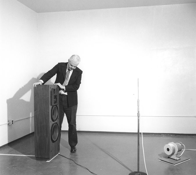
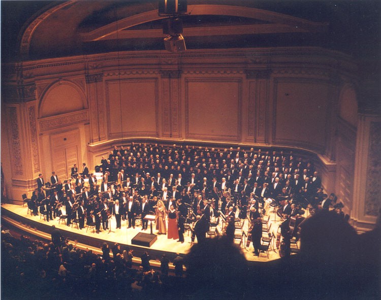

External references
License
GNU Free Documentation License
As of July 15, 2009 Wikibooks has moved to a dual-licensing system that supersedes the previous GFDL only licensing. In short, this means that text licensed under the GFDL only can no longer be imported to Wikibooks, retroactive to 1 November 2008. Additionally, Wikibooks text might or might not now be exportable under the GFDL depending on whether or not any content was added and not removed since July 15. |
Version 1.3, 3 November 2008 Copyright (C) 2000, 2001, 2002, 2007, 2008 Free Software Foundation, Inc. <http://fsf.org/>
Everyone is permitted to copy and distribute verbatim copies of this license document, but changing it is not allowed.
0. PREAMBLE
The purpose of this License is to make a manual, textbook, or other functional and useful document "free" in the sense of freedom: to assure everyone the effective freedom to copy and redistribute it, with or without modifying it, either commercially or noncommercially. Secondarily, this License preserves for the author and publisher a way to get credit for their work, while not being considered responsible for modifications made by others.
This License is a kind of "copyleft", which means that derivative works of the document must themselves be free in the same sense. It complements the GNU General Public License, which is a copyleft license designed for free software.
We have designed this License in order to use it for manuals for free software, because free software needs free documentation: a free program should come with manuals providing the same freedoms that the software does. But this License is not limited to software manuals; it can be used for any textual work, regardless of subject matter or whether it is published as a printed book. We recommend this License principally for works whose purpose is instruction or reference.
1. APPLICABILITY AND DEFINITIONS
This License applies to any manual or other work, in any medium, that contains a notice placed by the copyright holder saying it can be distributed under the terms of this License. Such a notice grants a world-wide, royalty-free license, unlimited in duration, to use that work under the conditions stated herein. The "Document", below, refers to any such manual or work. Any member of the public is a licensee, and is addressed as "you". You accept the license if you copy, modify or distribute the work in a way requiring permission under copyright law.
A "Modified Version" of the Document means any work containing the Document or a portion of it, either copied verbatim, or with modifications and/or translated into another language.
A "Secondary Section" is a named appendix or a front-matter section of the Document that deals exclusively with the relationship of the publishers or authors of the Document to the Document's overall subject (or to related matters) and contains nothing that could fall directly within that overall subject. (Thus, if the Document is in part a textbook of mathematics, a Secondary Section may not explain any mathematics.) The relationship could be a matter of historical connection with the subject or with related matters, or of legal, commercial, philosophical, ethical or political position regarding them.
The "Invariant Sections" are certain Secondary Sections whose titles are designated, as being those of Invariant Sections, in the notice that says that the Document is released under this License. If a section does not fit the above definition of Secondary then it is not allowed to be designated as Invariant. The Document may contain zero Invariant Sections. If the Document does not identify any Invariant Sections then there are none.
The "Cover Texts" are certain short passages of text that are listed, as Front-Cover Texts or Back-Cover Texts, in the notice that says that the Document is released under this License. A Front-Cover Text may be at most 5 words, and a Back-Cover Text may be at most 25 words.
A "Transparent" copy of the Document means a machine-readable copy, represented in a format whose specification is available to the general public, that is suitable for revising the document straightforwardly with generic text editors or (for images composed of pixels) generic paint programs or (for drawings) some widely available drawing editor, and that is suitable for input to text formatters or for automatic translation to a variety of formats suitable for input to text formatters. A copy made in an otherwise Transparent file format whose markup, or absence of markup, has been arranged to thwart or discourage subsequent modification by readers is not Transparent. An image format is not Transparent if used for any substantial amount of text. A copy that is not "Transparent" is called "Opaque".
Examples of suitable formats for Transparent copies include plain ASCII without markup, Texinfo input format, LaTeX input format, SGML or XML using a publicly available DTD, and standard-conforming simple HTML, PostScript or PDF designed for human modification. Examples of transparent image formats include PNG, XCF and JPG. Opaque formats include proprietary formats that can be read and edited only by proprietary word processors, SGML or XML for which the DTD and/or processing tools are not generally available, and the machine-generated HTML, PostScript or PDF produced by some word processors for output purposes only.
The "Title Page" means, for a printed book, the title page itself, plus such following pages as are needed to hold, legibly, the material this License requires to appear in the title page. For works in formats which do not have any title page as such, "Title Page" means the text near the most prominent appearance of the work's title, preceding the beginning of the body of the text.
The "publisher" means any person or entity that distributes copies of the Document to the public.
A section "Entitled XYZ" means a named subunit of the Document whose title either is precisely XYZ or contains XYZ in parentheses following text that translates XYZ in another language. (Here XYZ stands for a specific section name mentioned below, such as "Acknowledgements", "Dedications", "Endorsements", or "History".) To "Preserve the Title" of such a section when you modify the Document means that it remains a section "Entitled XYZ" according to this definition.
The Document may include Warranty Disclaimers next to the notice which states that this License applies to the Document. These Warranty Disclaimers are considered to be included by reference in this License, but only as regards disclaiming warranties: any other implication that these Warranty Disclaimers may have is void and has no effect on the meaning of this License.
2. VERBATIM COPYING
You may copy and distribute the Document in any medium, either commercially or noncommercially, provided that this License, the copyright notices, and the license notice saying this License applies to the Document are reproduced in all copies, and that you add no other conditions whatsoever to those of this License. You may not use technical measures to obstruct or control the reading or further copying of the copies you make or distribute. However, you may accept compensation in exchange for copies. If you distribute a large enough number of copies you must also follow the conditions in section 3.
You may also lend copies, under the same conditions stated above, and you may publicly display copies.
3. COPYING IN QUANTITY
If you publish printed copies (or copies in media that commonly have printed covers) of the Document, numbering more than 100, and the Document's license notice requires Cover Texts, you must enclose the copies in covers that carry, clearly and legibly, all these Cover Texts: Front-Cover Texts on the front cover, and Back-Cover Texts on the back cover. Both covers must also clearly and legibly identify you as the publisher of these copies. The front cover must present the full title with all words of the title equally prominent and visible. You may add other material on the covers in addition. Copying with changes limited to the covers, as long as they preserve the title of the Document and satisfy these conditions, can be treated as verbatim copying in other respects.
If the required texts for either cover are too voluminous to fit legibly, you should put the first ones listed (as many as fit reasonably) on the actual cover, and continue the rest onto adjacent pages.
If you publish or distribute Opaque copies of the Document numbering more than 100, you must either include a machine-readable Transparent copy along with each Opaque copy, or state in or with each Opaque copy a computer-network location from which the general network-using public has access to download using public-standard network protocols a complete Transparent copy of the Document, free of added material. If you use the latter option, you must take reasonably prudent steps, when you begin distribution of Opaque copies in quantity, to ensure that this Transparent copy will remain thus accessible at the stated location until at least one year after the last time you distribute an Opaque copy (directly or through your agents or retailers) of that edition to the public.
It is requested, but not required, that you contact the authors of the Document well before redistributing any large number of copies, to give them a chance to provide you with an updated version of the Document.
4. MODIFICATIONS
You may copy and distribute a Modified Version of the Document under the conditions of sections 2 and 3 above, provided that you release the Modified Version under precisely this License, with the Modified Version filling the role of the Document, thus licensing distribution and modification of the Modified Version to whoever possesses a copy of it. In addition, you must do these things in the Modified Version:
- Use in the Title Page (and on the covers, if any) a title distinct from that of the Document, and from those of previous versions (which should, if there were any, be listed in the History section of the Document). You may use the same title as a previous version if the original publisher of that version gives permission.
- List on the Title Page, as authors, one or more persons or entities responsible for authorship of the modifications in the Modified Version, together with at least five of the principal authors of the Document (all of its principal authors, if it has fewer than five), unless they release you from this requirement.
- State on the Title page the name of the publisher of the Modified Version, as the publisher.
- Preserve all the copyright notices of the Document.
- Add an appropriate copyright notice for your modifications adjacent to the other copyright notices.
- Include, immediately after the copyright notices, a license notice giving the public permission to use the Modified Version under the terms of this License, in the form shown in the Addendum below.
- Preserve in that license notice the full lists of Invariant Sections and required Cover Texts given in the Document's license notice.
- Include an unaltered copy of this License.
- Preserve the section Entitled "History", Preserve its Title, and add to it an item stating at least the title, year, new authors, and publisher of the Modified Version as given on the Title Page. If there is no section Entitled "History" in the Document, create one stating the title, year, authors, and publisher of the Document as given on its Title Page, then add an item describing the Modified Version as stated in the previous sentence.
- Preserve the network location, if any, given in the Document for public access to a Transparent copy of the Document, and likewise the network locations given in the Document for previous versions it was based on. These may be placed in the "History" section. You may omit a network location for a work that was published at least four years before the Document itself, or if the original publisher of the version it refers to gives permission.
- For any section Entitled "Acknowledgements" or "Dedications", Preserve the Title of the section, and preserve in the section all the substance and tone of each of the contributor acknowledgements and/or dedications given therein.
- Preserve all the Invariant Sections of the Document, unaltered in their text and in their titles. Section numbers or the equivalent are not considered part of the section titles.
- Delete any section Entitled "Endorsements". Such a section may not be included in the Modified version.
- Do not retitle any existing section to be Entitled "Endorsements" or to conflict in title with any Invariant Section.
- Preserve any Warranty Disclaimers.
If the Modified Version includes new front-matter sections or appendices that qualify as Secondary Sections and contain no material copied from the Document, you may at your option designate some or all of these sections as invariant. To do this, add their titles to the list of Invariant Sections in the Modified Version's license notice. These titles must be distinct from any other section titles.
You may add a section Entitled "Endorsements", provided it contains nothing but endorsements of your Modified Version by various parties—for example, statements of peer review or that the text has been approved by an organization as the authoritative definition of a standard.
You may add a passage of up to five words as a Front-Cover Text, and a passage of up to 25 words as a Back-Cover Text, to the end of the list of Cover Texts in the Modified Version. Only one passage of Front-Cover Text and one of Back-Cover Text may be added by (or through arrangements made by) any one entity. If the Document already includes a cover text for the same cover, previously added by you or by arrangement made by the same entity you are acting on behalf of, you may not add another; but you may replace the old one, on explicit permission from the previous publisher that added the old one.
The author(s) and publisher(s) of the Document do not by this License give permission to use their names for publicity for or to assert or imply endorsement of any Modified Version.
5. COMBINING DOCUMENTS
You may combine the Document with other documents released under this License, under the terms defined in section 4 above for modified versions, provided that you include in the combination all of the Invariant Sections of all of the original documents, unmodified, and list them all as Invariant Sections of your combined work in its license notice, and that you preserve all their Warranty Disclaimers.
The combined work need only contain one copy of this License, and multiple identical Invariant Sections may be replaced with a single copy. If there are multiple Invariant Sections with the same name but different contents, make the title of each such section unique by adding at the end of it, in parentheses, the name of the original author or publisher of that section if known, or else a unique number. Make the same adjustment to the section titles in the list of Invariant Sections in the license notice of the combined work.
In the combination, you must combine any sections Entitled "History" in the various original documents, forming one section Entitled "History"; likewise combine any sections Entitled "Acknowledgements", and any sections Entitled "Dedications". You must delete all sections Entitled "Endorsements".
6. COLLECTIONS OF DOCUMENTS
You may make a collection consisting of the Document and other documents released under this License, and replace the individual copies of this License in the various documents with a single copy that is included in the collection, provided that you follow the rules of this License for verbatim copying of each of the documents in all other respects.
You may extract a single document from such a collection, and distribute it individually under this License, provided you insert a copy of this License into the extracted document, and follow this License in all other respects regarding verbatim copying of that document.
7. AGGREGATION WITH INDEPENDENT WORKS
A compilation of the Document or its derivatives with other separate and independent documents or works, in or on a volume of a storage or distribution medium, is called an "aggregate" if the copyright resulting from the compilation is not used to limit the legal rights of the compilation's users beyond what the individual works permit. When the Document is included in an aggregate, this License does not apply to the other works in the aggregate which are not themselves derivative works of the Document.
If the Cover Text requirement of section 3 is applicable to these copies of the Document, then if the Document is less than one half of the entire aggregate, the Document's Cover Texts may be placed on covers that bracket the Document within the aggregate, or the electronic equivalent of covers if the Document is in electronic form. Otherwise they must appear on printed covers that bracket the whole aggregate.
8. TRANSLATION
Translation is considered a kind of modification, so you may distribute translations of the Document under the terms of section 4. Replacing Invariant Sections with translations requires special permission from their copyright holders, but you may include translations of some or all Invariant Sections in addition to the original versions of these Invariant Sections. You may include a translation of this License, and all the license notices in the Document, and any Warranty Disclaimers, provided that you also include the original English version of this License and the original versions of those notices and disclaimers. In case of a disagreement between the translation and the original version of this License or a notice or disclaimer, the original version will prevail.
If a section in the Document is Entitled "Acknowledgements", "Dedications", or "History", the requirement (section 4) to Preserve its Title (section 1) will typically require changing the actual title.
9. TERMINATION
You may not copy, modify, sublicense, or distribute the Document except as expressly provided under this License. Any attempt otherwise to copy, modify, sublicense, or distribute it is void, and will automatically terminate your rights under this License.
However, if you cease all violation of this License, then your license from a particular copyright holder is reinstated (a) provisionally, unless and until the copyright holder explicitly and finally terminates your license, and (b) permanently, if the copyright holder fails to notify you of the violation by some reasonable means prior to 60 days after the cessation.
Moreover, your license from a particular copyright holder is reinstated permanently if the copyright holder notifies you of the violation by some reasonable means, this is the first time you have received notice of violation of this License (for any work) from that copyright holder, and you cure the violation prior to 30 days after your receipt of the notice.
Termination of your rights under this section does not terminate the licenses of parties who have received copies or rights from you under this License. If your rights have been terminated and not permanently reinstated, receipt of a copy of some or all of the same material does not give you any rights to use it.
10. FUTURE REVISIONS OF THIS LICENSE
The Free Software Foundation may publish new, revised versions of the GNU Free Documentation License from time to time. Such new versions will be similar in spirit to the present version, but may differ in detail to address new problems or concerns. See http://www.gnu.org/copyleft/.
Each version of the License is given a distinguishing version number. If the Document specifies that a particular numbered version of this License "or any later version" applies to it, you have the option of following the terms and conditions either of that specified version or of any later version that has been published (not as a draft) by the Free Software Foundation. If the Document does not specify a version number of this License, you may choose any version ever published (not as a draft) by the Free Software Foundation. If the Document specifies that a proxy can decide which future versions of this License can be used, that proxy's public statement of acceptance of a version permanently authorizes you to choose that version for the Document.
11. RELICENSING
"Massive Multiauthor Collaboration Site" (or "MMC Site") means any World Wide Web server that publishes copyrightable works and also provides prominent facilities for anybody to edit those works. A public wiki that anybody can edit is an example of such a server. A "Massive Multiauthor Collaboration" (or "MMC") contained in the site means any set of copyrightable works thus published on the MMC site.
"CC-BY-SA" means the Creative Commons Attribution-Share Alike 3.0 license published by Creative Commons Corporation, a not-for-profit corporation with a principal place of business in San Francisco, California, as well as future copyleft versions of that license published by that same organization.
"Incorporate" means to publish or republish a Document, in whole or in part, as part of another Document.
An MMC is "eligible for relicensing" if it is licensed under this License, and if all works that were first published under this License somewhere other than this MMC, and subsequently incorporated in whole or in part into the MMC, (1) had no cover texts or invariant sections, and (2) were thus incorporated prior to November 1, 2008.
The operator of an MMC Site may republish an MMC contained in the site under CC-BY-SA on the same site at any time before August 1, 2009, provided the MMC is eligible for relicensing.
How to use this License for your documents
To use this License in a document you have written, include a copy of the License in the document and put the following copyright and license notices just after the title page:
- Copyright (c) YEAR YOUR NAME.
- Permission is granted to copy, distribute and/or modify this document
- under the terms of the GNU Free Documentation License, Version 1.3
- or any later version published by the Free Software Foundation;
- with no Invariant Sections, no Front-Cover Texts, and no Back-Cover Texts.
- A copy of the license is included in the section entitled "GNU
- Free Documentation License".
If you have Invariant Sections, Front-Cover Texts and Back-Cover Texts, replace the "with...Texts." line with this:
- with the Invariant Sections being LIST THEIR TITLES, with the
- Front-Cover Texts being LIST, and with the Back-Cover Texts being LIST.
If you have Invariant Sections without Cover Texts, or some other combination of the three, merge those two alternatives to suit the situation.
If your document contains nontrivial examples of program code, we recommend releasing these examples in parallel under your choice of free software license, such as the GNU General Public License, to permit their use in free software.