Sensory Systems/Print version
| This is the print version of Sensory Systems You won't see this message or any elements not part of the book's content when you print or preview this page. |
Table of contents
Introduction
Sensory Systems in Humans
- Visual System
- Auditory System
- Vestibular System
- Somatosensory System
- Olfactory System
- Gustatory System
Sensory Systems in Non-Primates
Appendix
The Wikibook of
Biological Organisms, an Engineer's Point of View.

From Wikibooks: The Free Library
Introduction
In order to survive - at least on the species level - we continually need to make decisions:
- "Should I cross the road?"
- "Should I run away from the creature in front of me?"
- "Should I eat the thing in front of me?"
- "Or should I try to mate it?"
To help us to make the right decision, and make that decision quickly, we have developed an elaborate system: a sensory system to notice what's going on around us; and a nervous system to handle all that information. And this system is big. Very big. Our nervous system contains about nerve cells (or neurons), and about 10-50 times as many supporting cells. These supporting cells, called gliacells, include oligodendrocytes, Schwann cells, and astrocytes. But do we really need all these cells?

Keep it simple: Unicellular Creatures
The answer is, "No!" We do not need that many cells in order to survive. Creatures existing of a single cell can be large, can respond to multiple stimuli, and can also be remarkably smart!
 |
 |
We often think of cells as really small things. But Xenophyophores (see image) are unicellular organisms that are found throughout the world's oceans and can get as large as 20 centimetres in diameter.
And even with this single cell, those organisms can respond to a number of stimuli. For example look at a creature from the group Paramecium: the paramecium is a group of unicellular ciliate protozoa formerly known as slipper animalcules, from their slipper shape. (The corresponding word in German is Pantoffeltierchen.) Despite the fact that these creatures consist of only one cell, they are able to respond to different environmental stimuli, e.g. to light or to touch.

And such unicellular organisms can be amazingly smart: the plasmodium of the slime mould Physarum polycephalum is a large amoebalike cell consisting of a dendritic network of tube-like structures. This single cell creature manages to connect sources finding the shortest connections (Nakagaki et al. 2000), and can even build efficient, robust and optimized network structures that resemble the Tokyo underground system (Tero et al. 2010). In addition, it has somehow developed the ability to read its tracks and tell if its been in a place before or not: this way it can save energy and not forage through locations where effort has already been put (Reid et al. 2012).
On the one hand, the approach used by the paramecium cannot be too bad, as they have been around for a long time. On the other hand, a single cell mechanism cannot be as flexible and as accurate in its responses as a more refined version of creatures, which use a dedicated, specialized system just for the registration of the environment: a Sensory System.
Not so simple: Three-hundred-and-two Neurons
While humans have hundreds of millions of sensory nerve cells, and about nerve cells, other creatures get away with significantly less. A famous one is Caenorhabditis elegans, a nematode with a total of 302 neurons.

C. elegans is one of the simplest organisms with a nervous system, and it was the first multicellular organism to have its genome completely sequenced. (The sequence was published in 1998.) And not only do we know its complete genome, we also know the connectivity between all 302 of its neurons. In fact, the developmental fate of every single somatic cell (959 in the adult hermaphrodite; 1031 in the adult male) has been mapped out. We know, for example, that only 2 of the 302 neurons are responsible for chemotaxis (“movement guided by chemical cues”, i.e. essentially smelling). Nevertheless, there is still a lot of research conducted—also on its smelling—in order to understand how its nervous system works.
General principles of Sensory Systems
Based on the example of the visual system, the general principle underlying our neuro-sensory system can be described as below:

All sensory systems are based on
- a Signal, i.e. a physical stimulus, provides information about our surrounding.
- the Collection of this signal, e.g. by using an ear or the lens of an eye.
- the Transduction of this stimulus into a nerve signal.
- the Processing of this information by our nervous system.
- And the generation of a resulting Action.
While the underlying physiology restricts the maximum frequency of our nerve-cells to about 1 kHz, more than one-million times slower than modern computers, our nervous system still manages to perform stunningly difficult tasks with apparent ease. The trick is there are lots of nerve cells (about ), and they are massively connected (one nerve cell can have up to 150,000 connections with other nerve cells).
Transduction
The role of our "senses" is to transduce relevant information from the world surrounding us into a type of signal that is understood by the next cells receiving that signal: the "Nervous System". (The sensory system is often regarded as part of the nervous system. Here I will try to keep these two apart, with the expression Sensory System referring to the stimulus transduction, and the Nervous System referring to the subsequent signal processing.)
Note here that only relevant information is to be transduced by the sensory system. The task of our senses is not to show us everything that is happening around us. Instead, their task is to filter out the important bits of the signals around us: electromagnetic signals, chemical signals, and mechanical ones. Our Sensory Systems transduce those environmental variables that are (probably) important to us. And the Nervous System propagates them in such a way that the responses that we take help us to survive, and to pass on our genes.
Types of sensory transducers
- Mechanical receptors
- Balance system (vestibular system)
- Hearing (auditory system)
- Pressure:
- Fast adaptation (Meissner’s corpuscle, Pacinian corpuscle) ? movement
- Slow adaptation (Merkel disks, Ruffini endings) ? shape Comment: these signals are transferred fast
- Muscle spindles
- Golgi organs: in the tendons
- Joint-receptors
- Chemical receptors
- Smell (olfactory system)
- Taste
- Light-receptors (visual system): here we have light-dark receptors (rods), and three different color receptors (cones)
- Thermo-receptors
- Heat-sensors (maximum sensitivity at ~ 45°C, signal temperatures < 50°C)
- Cold-sensors (maximum sensitivity at ~ 25°C, signal temperatures > 5°C)
- Comment: The information processing of these signals is similar to those of visual color signals, and is based on differential activity of the two sensors; these signals are slow
- Electro-receptors: for example in the bill of the platypus
- Magneto-receptors
- Pain receptors (nocioceptors): pain receptors are also responsible for itching; these signals are passed on slowly.
Neurons
What distinguishes neurons from other cells in the human body, like liver cells or fat cells? Neurons are unique, in that they:
- can switch quickly between two states (which can also be done by muscle cells);
- can propagate this change into a specified direction and over longer distances (which cannot be done by muscle cells);
- and this state-change can be signaled effectively to other connected neurons.
While there are more than 50 distinctly different types of neurons, they all share the same structure:

- An input stage, often called dendrites, as the input-area often spreads out like the branches of a tree. Input can come from sensory cells or from other neurons; it can come from a single cell (e.g. a bipolar cell in the retina receives input from a single cone), or from up to 150’000 other neurons (e.g. Purkinje cells in the Cerebellum); and it can be positive (excitatory) or negative (inhibitory).
- An integrative stage: the cell body does the household chores (generating the energy, cleaning up, generating the required chemical substances, etc), combines the incoming signals, and determines when to pass a signal on down the line.
- A conductile stage, the axon: once the cell body has decided to send out a signal, an action potential propagates along the axon, away from the cell body. An action potential is a quick change in the state of a neuron, which lasts for about 1 msec. Note that this defines a clear direction in the signal propagation, from the cell body, to the:
- output stage: The output is provided by synapses, i.e. the points where a neuron contacts the next neuron down the line, most often by the emission of neurotransmitters (i.e. chemicals that affect other neurons) which then provide an input to the next neuron.
Principles of Information Processing in the Nervous System
Parallel processing
An important principle in the processing of neural signals is parallelism. Signals from different locations have different meaning. This feature, sometimes also referred to as line labeling, is used by the
- Auditory system - to signal frequency
- Olfactory system - to signal sweet or sour
- Visual system - to signal the location of a visual signal
- Vestibular system - to signal different orientations and movements
Population Coding
Sensory information is rarely based on the signal nerve. It is typically coded by different patterns of activity in a population of neurons. This principle can be found in all our sensory systems.
Learning
The structure of the connections between nerve cells is not static. Instead it can be modified, to incorporate experiences that we have made. Thereby nature walks a thin line:
_(14562557107).jpg)
- If we learn too slowly, we might not make it. One example is the "Passenger Pidgeon", an American bird which is extinct by now. In the last century (and the one before), this bird was shot in large numbers. The mistake of the bird was: when some of them were shot, the others turned around, maybe to see what's up. So they were shot in turn - until the birds were essentially gone. The lesson: if you learn too slowly (i.e. to run away when all your mates are killed), your species might not make it.

- On the other hand, we must not learn too fast, either. For example, the monarch butterfly migrates. But it takes them so long to get from "start" to "finish", that the migration cannot be done by one butterfly alone. In other words, no single butterfly makes the whole journey. Nevertheless, the genetic disposition still tells the butterflies where to go, and when they are there. If they would learn any faster - they could never store the necessary information in their genes. In contrast to other cells in the human body, nerve cells are not re-generated in the human body.
Simulation of Neural Systems
Simulating Action Potentials
Action Potential
The "action potential" is the stereotypical voltage change that is used to propagate signals in the nervous system.

With the mechanisms described below, an incoming stimulus (of any sort) can lead to a change in the voltage potential of a nerve cell. Up to a certain threshold, that's all there is to it ("Failed initiations" in Fig. 4). But when the Threshold of voltage-gated ion channels is reached, it comes to a feed-back reaction that almost immediately completely opens the Na+-ion channels ("Depolarization" below): This reaches a point where the permeability for Na+ (which is in the resting state is about 1% of the permeability of K+) is 20\*larger than that of K+. Together, the voltage rises from about -60mV to about +50mV. At that point internal reactions start to close (and block) the Na+ channels, and open the K+ channels to restore the equilibrium state. During this "Refractory period" of about 1 m, no depolarization can elicit an action potential. Only when the resting state is reached can new action potentials be triggered.
To simulate an action potential, we first have to define the different elements of the cell membrane, and how to describe them analytically.
Cell Membrane
The cell membrane is made up by a water-repelling, almost impermeable double-layer of proteins, the cell membrane. The real power in processing signals does not come from the cell membrane, but from ion channels that are embedded into that membrane. Ion channels are proteins which are embedded into the cell membrane, and which can selectively be opened for certain types of ions. (This selectivity is achieved by the geometrical arrangement of the amino acids which make up the ion channels.) In addition to the Na+ and K+ ions mentioned above, ions that are typically found in the nervous system are the cations Ca2+, Mg2+, and the anions Cl- .
States of ion channels
Ion channels can take on one of three states:
- Open (For example, an open Na-channel lets Na+ ions pass, but blocks all other types of ions).
- Closed, with the option to open up.
- Closed, unconditionally.
Resting state
The typical default situation – when nothing is happening - is characterized by K+ that are open, and the other channels closed. In that case two forces determine the cell voltage:
- The (chemical) concentration difference between the intra-cellular and extra-cellular concentration of K+, which is created by the continuous activity of the ion pumps described above.
- The (electrical) voltage difference between the inside and outside of the cell.
The equilibrium is defined by the Nernst-equation:
![{\displaystyle {{E}_{X}}={\frac {RT}{zF}}\ln {\frac {{[X]}_{o}}{{[X]}_{i}}}}](https://wikimedia.org/api/rest_v1/media/math/render/svg/5e2d5c294b8784f463d80357bd660f5e515b23a8)
R ... gas-constant, T ... temperature, z ... ion-valence, F ... Faraday constant, [X]o/i … ion concentration outside/ inside. At 25° C, RT/F is 25 mV, which leads to a resting voltage of
![{\displaystyle {{E}_{X}}={\frac {25mV}{z}}\log {\frac {{[X]}_{o}}{{[X]}_{i}}}}](https://wikimedia.org/api/rest_v1/media/math/render/svg/49ea1afb0f8c662cb48929a3da01c5acdd4d6f88)
With typical K+ concentration inside and outside of neurons, this yields . If the ion channels for K+, Na+ and Cl- are considered simultaneously, the equilibrium situation is characterized by the Goldman-equation

![{\displaystyle {{V}_{m}}={\frac {RT}{F}}\ln {\frac {{{P}_{K}}{{[{{K}^{+}}]}_{o}}+{{P}_{Na}}{{[N{{a}^{+}}]}_{o}}+{{P}_{Cl}}{{[Cl-]}_{i}}}{{{P}_{K}}{{[{{K}^{+}}]}_{i}}+{{P}_{Na}}{{[N{{a}^{+}}]}_{i}}+{{P}_{Cl}}{{[Cl-]}_{o}}}}}](https://wikimedia.org/api/rest_v1/media/math/render/svg/5a99888fc4b3f0858a0551a76f813fa566c3c7e2)
where Pi denotes the permeability of Ion "i", and I the concentration. Using typical ion concentration, the cell has in its resting state a negative polarity of about -60 mV.
Activation of Ion Channels
The nifty feature of the ion channels is the fact that their permeability can be changed by
- A mechanical stimulus (mechanically activated ion channels)
- A chemical stimulus (ligand activated ion channels)
- Or an by an external voltage (voltage gated ion channels)
- Occasionally ion channels directly connect two cells, in which case they are called gap junction channels.
Important
- Sensory systems are essentially based ion channels, which are activated by a mechanical stimulus (pressure, sound, movement), a chemical stimulus (taste, smell), or an electromagnetic stimulus (light), and produce a "neural signal", i.e. a voltage change in a nerve cell.
- Action potentials use voltage gated ion channels, to change the "state" of the neuron quickly and reliably.
- The communication between nerve cells predominantly uses ion channels that are activated by neurotransmitters, i.e. chemicals emitted at a synapse by the preceding neuron. This provides the maximum flexibility in the processing of neural signals.
Modeling a voltage dependent ion channel
Ohm's law relates the resistance of a resistor, R, to the current it passes, I, and the voltage drop across the resistor, V:

or

where is the conductance of the resistor. If you now suppose that the conductance is directly proportional to the probability that the channel is in the open conformation, then this equation becomes


where is the maximum conductance of the cannel, and is the probability that the channel is in the open conformation.


Example: the K-channel
Voltage gated potassium channels (Kv) can be only open or closed. Let α be the rate the channel goes from closed to open, and β the rate the channel goes from open to closed

Since n is the probability that the channel is open, the probability that the channel is closed has to be (1-n), since all channels are either open or closed. Changes in the conformation of the channel can therefore be described by the formula

Note that α and β are voltage dependent! With a technique called "voltage-clamping", Hodgkin and Huxley determine these rates in 1952, and they came up with something like

If you only want to model a voltage-dependent potassium channel, these would be the equations to start from. (For voltage gated Na channels, the equations are a bit more difficult, since those channels have three possible conformations: open, closed, and inactive.)
Hodgkin Huxley equation
The feedback-loop of voltage-gated ion channels mentioned above made it difficult to determine their exact behaviour. In a first approximation, the shape of the action potential can be explained by analyzing the electrical circuit of a single axonal compartment of a neuron, consisting of the following components: 1) Na channel, 2) K channel, 3) Cl channel, 4) leakage current, 5) membrane capacitance, :

The final equations in the original Hodgkin-Huxley model, where the currents in of chloride ions and other leakage currents were combined, were as follows:


where , , and are time- and voltage dependent functions which describe the membrane-permeability. For example, for the K channels n obeys the equations described above, which were determined experimentally with voltage-clamping. These equations describe the shape and propagation of the action potential with high accuracy! The model can be solved easily with open source tools, e.g. the Python Dynamical Systems Toolbox PyDSTools. A simple solution file is available under [1] , and the output is shown below.


Links to full Hodgkin-Huxley model
Modeling the Action Potential Generation: The Fitzhugh-Nagumo model

The Hodgkin-Huxley model has four dynamical variables: the voltage , the probability that the K channel is open, , the probability that the Na channel is open given that it was closed previously, , and the probability that the Na channel is open given that it was inactive previously, . A simplified model of action potential generation in neurons is the Fitzhugh-Nagumo (FN) model. Unlike the Hodgkin-Huxley model, the FN model has only two dynamic variables, by combining the variables and into a single variable , and combining the variables and into a single variable


The following two examples are taken from I is an external current injected into the neuron. Since the FN model has only two dynamic variables, its full dynamics can be explored using phase plane methods (Sample solution in Python here [2])

Simulating a Single Neuron with Positive Feedback
The following two examples are taken from [3] . This book provides a fantastic introduction into modeling simple neural systems, and gives a good understanding of the underlying information processing.

Let us first look at the response of a single neuron, with an input , and with feedback onto itself. The weight of the input is , and the weight of the feedback . The response of the neuron is given by


This shows how already very simple simulations can capture signal processing properties of real neurons.

""" Simulation of the effect of feedback on a single neuron """

import numpy as np
import matplotlib.pylab as plt

# System configuration
is_impulse = True   # 'True' for impulse, 'False' for step
t_start = 11        # set a start time for the input
n_steps = 100
v = 1               # input weight
w = 0.95            # feedback weight

# Stimulus
x = np.zeros(n_steps)
if is_impulse:
    x[t_start] = 1  # then set the input at only one time point
else:
    x[t_start:] = 1 # step input

# Response
y = np.zeros(n_steps)           # allocate output vector
for t in range(1, n_steps):     # at every time step (skipping first)
    y[t] = w*y[t-1] + v*x[t-1]  # compute the output

# Plot the results
time = np.arange(n_steps)
fig, axs = plt.subplots(2, 1, sharex=True)

axs[0].plot(time, x)
axs[0].set_ylabel('Input')
axs[0].margins(x=0)

axs[1].plot(time, y)
axs[1].set_xlabel('Time Step')
axs[1].set_ylabel('Output')

plt.show()
Simulating a Simple Neural System
Even very simple neural systems can display a surprisingly versatile set of behaviors. An example is Wilson's model of the locust-flight central pattern generator. Here the system is described by

W is the connection matrix describing the recurrent connections of the neurons, and describes the input to the system.


""" 'Recurrent' feedback in simple network:
linear version of Wilson's locust flight central pattern generator (CPG) """

import numpy as np
import matplotlib.pylab as plt

# System configuration
v = np.zeros(4)                     # input weight matrix (vector)
v[1] = 1

w1 = [  0.9,  0.2,    0,     0]     # feedback weights to unit one
w2 = [-0.95,  0.4, -0.5,     0]     # ... to unit two
w3 = [    0, -0.5,  0.4, -0.95]     # ... to unit three
w4 = [    0,    0,  0.2,  0.9 ]     # ... to unit four
W = np.vstack( [w1, w2, w3, w4] )

n_steps = 100

# Initial kick, to start the system
x = np.zeros(n_steps)               # zero input vector
t_kick = 11
x[t_kick] = 1

# Simulation
y = np.zeros( (4,n_steps) )         # zero output vector
for t in range(1,n_steps):          # for each time step
    y[:,t] = W @ y[:,t-1] + v * x[t-1]  # compute output

# Show the result
time = np.arange(n_steps)
plt.plot(time, x, '-', label='Input')
plt.plot(time, y[1,:], ls='dashed', label = 'Left Motorneuron')
plt.plot(time, y[2,:], ls='dotted', label='Right Motorneuron')

# Format the plot
plt.xlabel('Time Step')
plt.ylabel('Input and Unit Responses')
plt.gca().margins(x=0)
plt.tight_layout()
plt.legend()
plt.show()
The Development and Theory of Neuromorphic Circuits
Introduction
Neurmomorphic engineering uses very-large-scale-integration (VLSI) systems to build analog and digital circuits, emulating neuro-biological architecture and behavior. Most modern circuitry primarily utilizes digital circuit components because they are fast, precise, and insensitive to noise. Unlike more biologically relevant analog circuits, digital circuits require higher power supplies and are not capable of parallel computing. Biological neuron behaviors, such as membrane leakage and threshold constraints, are functions of material substrate parameters, and require analog systems to model and fine tune beyond digital 0/1. This paper will briefly summarize such neuromorphic circuits, and the theory behind their analog circuit components.
Current Events in Neuromorphic Engineering
In the last 10 years, the field of neuromorphic engineering has experienced a rapid upswing and received strong attention from the press and the scientific community.
After this topic came to the attention of the EU Commission, the Human Brain Project was launched in 2013, which was funded with 600 million euros over a period of ten years. The aim of the project is to simulate the human brain from the level of molecules and neurons to neural circuits. It is scheduled to end in September 2023, and although the main goal has not been achieved, it is providing detailed 3D maps of at least 200 brain regions and supercomputers to model functions such as memory and consciousness, among other things [4]. Another major deliverable is the EBRAINS virtual platform, launched in 2019. It provides a set of tools and image data that scientists worldwide can use for simulations and digital experiments.
Also in 2013, the U.S. National Institute of Health announced funding announced funding for the BRAIN project aimed at reconstructing the activity of large populations of neurons. It is ongoing and $680 million in funding has been allocated through 2023.
Other major accomplishments in recent years are listed below
1. TrueNorth Chip (IBM, 2014): with a total number of 268 million programmable synapses
2. Loihi Chip (Intel, 2017): based on asynchronous neural spiking network (SNN) for adaptive event-driven parallel computing. It was superseded by Loihi2 in 2021.
3. prototype chip (IMEC, 2017): first self-learning neuromorphic chip based on OxRAM technology
4. Akida AI Processor Development Kits (Brainchip, 2021): 1st commercially available neuromorphic processor
Transistor Structure & Physics
Metal-oxide-silicon-field-effect-transistors (MOSFETs) are common components of modern integrated circuits. MOSFETs are classified as unipolar devices because each transistor utilizes only one carrier type; negative-type MOFETs (nFETs) have electrons as carriers and positive-type MOSFETs (pFETs) have holes as carriers.

The general MOSFET has a metal gate (G), and two pn junction diodes known as the source (S) and the drain (D) as shown in Fig \ref{fig: transistor}. There is an insulating oxide layer that separates the gate from the silicon bulk (B). The channel that carries the charge runs directly below this oxide layer. The current is a function of the gate dimensions.
The source and the drain are symmetric and differ only in the biases applied to them. In a nFET device, the wells that form the source and drain are n-type and sit in a p-type substrate. The substrate is biased through the bulk p-type well contact. The positive current flows below the gate in the channel from the drain to the source. The source is called as such because it is the source of the electrons. Conversely, in a pFET device, the p-type source and drain are in a bulk n-well that is in a p-type substrate; current flows from the source to the drain.
When the carriers move due to a concentration gradient, this is called diffusion. If the carriers are swept due to an electric field, this is called drift. By convention, the nFET drain is biased at a higher potential than the source, whereas the source is biased higher in a pFET.
In a nFET, when a positive voltage is applied to the gate, positive charge accumulates on the metal contact. This draws electrons from the bulk to the silicon-oxide interface, creating a negatively charged channel between the source and the drain. The larger the gate voltage, the thicker the channel becomes which reduces the internal resistance, and thus increases the current logarithmically. For small gate voltages, typically below the threshold voltage, , the channel is not yet fully conducting and the increase in current from the drain to the source increases linearly on a logarithmic scale. This regime, when , is called the subthreshold region. Beyond this threshold voltage, , the channel is fully conducting between the source and drain, and the current is in the superthreshold regime.


For current to flow from the drain to the source, there must initially be an electric field to sweep the carriers across the channel. The strength of this electric field is a function of the applied potential difference between the source and the drain (), and thus controls the drain-source current. For small values of , the current linearly increases as a function of for constant values. As increases beyond , the current saturates.


pFETs behave similarly to nFET except that the carriers are holes, and the contact biases are negated.
In digital applications, transistors either operate in their saturation region (on) or are off. This large range in potential differences between the on and off modes is why digital circuits have such a high power demand. Contrarily, analog circuits take advantage of the linear region of transistors to produce a continuous signals with a lower power demand. However, because small changes in gate or source-drain voltages can create a large change in current, analog systems are prone to noise.
The field of neuromorphic engineering takes advantage of the noisy nature of analog circuits to replicate stochastic neuronal behavior [5] [6]. Unlike clocked digital circuits, analog circuits are capable of creating action potentials with temporal dynamics similar to biological time scales (approx. ). The potentials are slowed down and firing rates are controlled by lengthening time constants through leaking biases and variable resistive transistors. Analog circuits have been created that are capable of emulating biological action potentials with varying temporal dynamics, thus allowing silicon circuits to mimic neuronal spike-based learning behavior [7]. Whereas, digital circuits can only contain binary synaptic weights [0,1], analog circuits are capable of maintaining synaptic weights within a continuous range of values, making analog circuits particularly advantageous for neuromorophic circuits.

Basic static circuits
With an understanding of how transistors work and how they are biased, basic static analog circuits can be rationalized through. Afterward, these basic static circuits will be combined to create neuromorphic circuits. In the following circuit examples, the source, drain, and gate voltages are fixed, and the current is the output. In practice, the bias gate voltage is fixed to a subthreshold value (), the drain is held in saturation (), and the source and bulk are tied to ground (, ). All non-idealities are ignored.


Diode-Connected Transistor
A diode-connected nFET has its gate tied to the drain. Since the floating drain controls the gate voltage, the drain-gate voltages will self-regulate so the device will always sink the input current, . Beyond several microvolts, the transistor will run in saturation. Similarly, a diode-connected pFET has its gate tied to the source. Though this simple device seems to merely function as a short circuit, it is commonly used in analog circuits for copying and regulating current. Particularly in neuromorphic circuits, they are used to slow current sinks, to increase circuit time constants to biologically plausible time regimes.

Current Mirror
A current mirror takes advantage of the diode-connected transistor’s ability to sink current. When an input current is forced through the diode connected transistor, , the floating drain and gate are regulated to the appropriate voltage that allows the input current to pass. Since the two transistors share a common gate node, will also sink the same current. This forces the output transistor to duplicate the input current. The output will mirror the input current as long as:


- .


The current mirror gain can be controlled by adjusting these two parameters. When using transistors with different dimensions, otherwise known as a tilted mirror, the gain is:

A pFET current mirror is simply a flipped nFET mirror, where the diode-connected pFET mirrors the input current, and forces the other pFET to source output current.
Current mirrors are commonly used to copy currents without draining the input current. This is especially essential for feedback loops, such as the one use to accelerate action potentials, and summing input currents at a synapse.
Source Follower
A source follower consists of an input transistor, , stacked on top of a bias transistor, . The fixed subthreshold () bias voltage controls the gate , forcing it to sink a constant current, . is thus also forced to sink the same current () regardless of what the input voltage, .


A source follower is called so because the output, , will follow with a slight offset described by:

where kappa is the subthreshold slope factor, typically less than one.

This simple circuit is often used as a buffer. Since no current can flow through the gate, this circuit will not draw current from the input, an important trait for low-power circuits. Source followers can also isolate circuits, protecting them from power surges or static. A pFET source follower only differs from an nFET source follower in that the bias pFET has its bulk tied to .
In neuromorphic circuits, source followers and the like are used as simple current integrators which behave like post-synaptic neurons collecting current from many pre-synaptic neurons.
Inverter
An inverter consists of a pFET, , stacked on top of a nFET, , with their gates tied to the input, and the output is tied to the common source node, . When a high signal is input, the pFET is off but the nFET is on, effectively draining the output node, , and inverting the signal. Contrarily, when the input signal is low, the nFET is off but the pFET is on, charging up the node.

This simple circuit is effective as a quick switch. The inverter is also commonly used as a buffer because an output current can be produced without directly sourcing the input current, as no current is allowed through the gate. When two inverters are used in series, they can be used as a non-inverting amplifier. This was used in the original Integrate-and-Fire silicon neuron by Mead et al., 1989 to create a fast depolarizing spike similar to that of a biological action potential [8]. However, when the input fluctuates between high and low signals both transistors are in superthreshold saturation draining current, making this a very power hungry circuit.
Current Conveyor
The current conveyor is also commonly known as a buffered current mirror. Consisting of two transistors with their gates tied to a node of the other, the Current Conveyor self regulates so that the output current matches the input current, in a manner similar to the Current Mirror.
The current conveyor is often used in place of current mirrors for large serially repetitious arrays. This is because the current mirror current is controlled through the gate, whose oxide capacitance will result in a delayed output. Though this lag is negligible for a single output current mirror, long mirroring arrays will accumulative significant output delays. Such delays would greatly hinder large parallel processes such as those that try to emulate biological neural network computational strategies.
Differential Pair
The differential pair is a comparative circuit composed of two source followers with a common bias that forces the current of the weaker input to be silenced. The bias transistor will force to remain constant, tying the common node, , to a fixed voltage. Both input transistors will want to drain current proportional to their input voltages, and , respectively. However, since the common node must remain fixed, the drains of the input transistors must raise in proportion to the gate voltages. The transistor with the lower input voltage will act as a choke and allow less current through its drain. The losing transistor will see its source voltage increase and thus fall out of saturation.


The differential pair, in the setting of a neuronal circuit, can function as an activation threshold of an ion channel below which the voltage-gated ion channel will not open, preventing the neuron from spiking [9].
Silicon neurons
Winner-Take-All
The Winner-Take-All (WTA) circuit, originally designed by Lazzaro et al. [10], is a continuous time, analog circuit. It compares the outputs of an array of cells, and only allows the cell with the highest output current to be on, inhibiting all other competing cells.

Each cell comprises a current-controlled conveyor, and receives input currents, and outputs into a common line controlling a bias transistor. The cell with the largest input current, will also output the largest current, increasing the voltage of the common node. This forces the weaker cells to turn off. The WTA circuit can be extended to include a large network of competing cells. A soft WTA also has its output current mirrored back to the input, effectively increasing the cell gain. This is necessary to reduce noise and random switching if the cell array has a small dynamic range.
WTA networks are commonly used as a form of competitive learning in computational neural networks that involve distributed decision making. In particular, WTA networks have been used to perform low level recognition and classification tasks that more closely resemble cortical activity during visual selection tasks [11].
Integrate & Fire Neuron
The most general schematic of an Integrate & Fire Neuron, is also known as an Axon-Hillock Neuron, is the most commonly used spiking neuron model [8]. Common elements between most Axon-Hillock circuits include: a node with a memory of the membrane potential , an amplifier, a positive feedback loop , and a mechanism to reset the membrane potential to its resting state, .


The input current, , charges the , which is stored in a capacitor, C. This capacitor is analogous to the lipid cellular membrane which prevents free ionic diffusion, creating the membrane potential from the accumulated charge difference on either side of the lipid membrane. The input is amplified to output a voltage spike. A change in membrane potential is positively fed back through to , producing a faster spike. This closely resembles how a biological axon hillock, which is densely packed with voltage-gated sodium channels, amplifies the summed potentials to produce an action potential. When a voltage spike is produced, the reset bias, , begins to drain the node. This is similar to sodium-potassium channels which actively pump sodium and potassium ions against the concentration gradient to maintain the resting membrane potential.


The original Axon Hillock silicon neuron has been adapted to include an activation threshold with the addition of a Differential Pair comparing the input to a set threshold bias [9]. This conductance-based silicon neuron utilizes differential-pair integrator (DPI) with a leaky transistor to compare the input, to the threshold, . The leak bias , refractory period bias , adaptation bias , and positive feed back gain, all independently control the spiking frequency. Research has been focused on implementing spike frequency adaptation to set refractory periods and modulating thresholds [12]. Adaptation allows for the neuron to modulate its output firing rate as a function of its input. If there is a constant high frequency input, the neuron will be desensitized to the input and the output will be steadily diminished over time. The adaptive component of the conductance-based neuron circuit is modeled through the calcium flux and stores the memory of past activity through the adaptive capacitor, . The advent of spike frequency adaptation allowed for changes on the neuron level to control adaptive learning mechanisms on the synapse level. This model of neuronal learning is modeled from biology [13] and will be further discussed in Silicon Synapses.


Silicon Synapses
The most basic silicon synapse, originally used by Mead et al.,1989 [8], simply consists of a pFET source follower that receives a low signal pulse input and outputs a unidirectional current, [14].


The amplitude of the spike is controlled by the weight bias, , and the pulse width is directly correlated with the input pulse width which is set by $V_{\tau}$. The capacitor in the Lazzaro et al. (1993) synapse circuit was added to increase the spike time constant to a biologically plausible value. This slowed the rate at which the pulse hyperpolarizes and depolarizes, and is a function of the capacitance.


For multiple inputs depicting competitive excitatory and inhibitive behavior, the log-domain integrator uses and to regulate the output current magnitude, , as function of the input current, , according to:

controls the rate at which is able to charge the output transistor gate. governs the rate in which the output is sunk. This competitive nature is necessary to mimic biological behavior of neurotransmitters that either promote or depress neuronal firing.
Synaptic models have also been developed with first order linear integrators using log-domain filters capable of modeling the exponential decay of excitatory post-synaptic current (EPSC) [15]. This is necessary to have biologically plausible spike contours and time constants. The gain is also independently controlled from the synapse time constant which is necessary for spike-rate and spike-timing dependent learning mechanisms.

The aforementioned synapses simply relay currents from the pre-synaptic sources, varying the shape of the pulse spike along the way. They do not, however, contain any memory of previous spikes, nor are they capable of adapting their behavior according to temporal dynamics. These abilities, however, are necessary if neuromorphic circuits are to learn like biological neural networks.


According to Hebb's postulate, behaviors like learning and memory are hypothesized to occur on the synaptic level [16]. It accredits the learning process to long-term neuronal adaptation in which pre- and post-synaptic contributions are strengthened or weakened by biochemical modifications. This theory is often summarized in the saying, "Neurons that fire together, wire together." Artificial neural networks model learning through these biochemical "wiring" modifications with a single parameter, the synaptic weight, . A synaptic weight is a parameter state variable that quantifies how a presynaptic neuron spike affects a postsynaptic neuron output. Two models of Hebbian synaptic weight plasticity include spike-rate-dependent plasticity (SRDP), and spike-timing-dependent plasticity (STDP). Since the conception of this theory, biological neuron activity has been shown to exhibit behavior closely modeling Hebbian learning. One such example is of synaptic NMDA and AMPA receptor plastic modifications that lead to calcium flux induced adaptation [17].
Learning and long-term memory of information in biological neurons is accredited to NMDA channel induced adaptation. These NMDA receptors are voltage dependent and control intracellular calcium ion flux. It has been shown in animal studies that neuronal desensitization is diminished when extracellular calcium was reduced [17].


Since calcium concentration exponentially decays, this behavior easily implemented on hardware using subthreshold transistors. A circuit model demonstrating calcium dependent biological behavior is shown by Rachmuth et al. (2011) [18]. The calcium signal, , regulates AMPA and NMDA channel activity through the node according to calcium-dependent STDP and SRDP learning rules. The output of these learning rules is the synaptic weight, , which is proportional to the number of active AMPA and NMDA channels. The SRDP model describes the weight in terms of two state variables, , which controls the update rule, and , which controls the learning rate.


where is the synaptic weight, is the update rule, is the learning rate, and is a constant that allows the weight to drift out of saturation in absence of an input.
![{\displaystyle dw=\eta ([Ca_{2+}])\cdot (\Omega ([Ca_{2+}])-\lambda w),}](https://wikimedia.org/api/rest_v1/media/math/render/svg/5c904f8985f83bcc0f7cfbb240a97f5b6db16b3e)
![{\displaystyle \Omega ([Ca_{2+}])}](https://wikimedia.org/api/rest_v1/media/math/render/svg/b8365820f3ba6b3eb8631a0bb5ce819be1ec17d1)
![{\displaystyle \eta ([Ca_{2+}])}](https://wikimedia.org/api/rest_v1/media/math/render/svg/d9d4224f92cfee5905b380eb00eff81b77a2fe12)

The NMDA channel controls the calcium influx, . The NMDA receptor voltage-dependency is modeled by , and the channel mechanics are controlled with a large capacitor to increase the calcium time constant, . The output is copied via current mirrors into the and circuits to perform downstream learning functions.


The circuit compares to threshold biases, and ), that respectively control long-term potentiation or long-term depression through a series of differential pair circuits. The output of differential pairs determines the update rule. This circuit has been demonstrated to exhibit various Hebbian learning rules as observed in the hippocampus, and anti-Hebbian learning rules used in the cerebellum.


The circuit controls when synaptic learning can occur by only allowing updates when is above a differential pair set threshold, . The learning rate (LR) is modeled according to:

where is a function of and controls the learning rate, is the capacitance of the circuit, and is the threshold voltage of the comparator. This function demonstrates that must be biased to maintain an elevated in order to simulate SRDT. A leakage current, , was included to drain to during inactivity.
![{\displaystyle \tau _{LR}\sim {\frac {\theta _{\eta }\cdot C_{\eta }}{I_{\eta }\cdot [Ca_{2+}]}},}](https://wikimedia.org/api/rest_v1/media/math/render/svg/20bac65985bece7edd0e340742a5312609aa49b9)
![{\displaystyle [Ca_{2+}]}](https://wikimedia.org/api/rest_v1/media/math/render/svg/d4caea324562bc2c0bd11d4c73ed9eea47405b55)


The NEURON simulation environment
Introduction
Neuron is a simulation environment with which you can simulate the propagation of ions and action potentials in biological and artificial neurons as well as in networks of neurons [19]. The user can specify a model geometry by defining and connecting neuron cell parts, which can be equipped with various mechanisms such as ion channels, clamps and synapses. To interact with NEURON the user can either use the graphical user interface (GUI) or one of the programming languages hoc (a language with a C like syntax) or Python as an interpreter. The GUI contains a wide selection of the most-used features, an example screenshot is shown in the Figure on the right. The programming languages on the other hand can be exploited to add more specific mechanisms to the model and for automation purposes Furthermore, custom mechanisms can be created with the programming language NMODL, which is an extension to MODL, a model description language developed by the NBSR (National Biomedical Simulation Resource). These new mechanisms can then be compiled, and added to models through the GUI or interpreters.

Neuron was initially developed by John W. Moore at Duke university in collaboration with Michael Hines. It is currently used in numerous institutes and universities for educational and research purposes. There is an extensive amount of information available including the official website containing the documentation, the NEURON forum and various tutorials and guides. Furthermore in 2006 the authoritative reference book for NEURON was published called “The NEURON Book” [20]. To read the following chapters and to work with NEURON, some background knowledge on the physiology of neurons is recommended. Some examples of information sources about neurons are the WikiBook chapter, or the videos in the introduction of the Advanced Nervous System Physiology chapter on Khan academy. We will not cover specific commands or details about how to perform the here mentioned actions with NEURON since this document is not intended to be a tutorial but only an overview of the possibilities and model structure within NEURON. For more practical information on the implementation with NEURON I would recommend the tutorials which are linked below and the documentation on the official webpage [19].
Model creation

Single Cell Geometry
First we will discuss the creation of a model geometry that consists of a single biological neuron. A schematic representation of a Neuron is shown in the Figure on the right. In the following Listing an example code snippet is shown in which a multi-compartment cell with one soma and two dendrites is specified using hoc.

load_file("nrngui.hoc")

// Create a soma object and an array containing 2 dendrite objects
ndend = 2
create soma, dend[ndend]
access soma

// Initialize the soma and the dendrites
soma {
  nseg = 1
  diam = 18.8
  L = 18.8
  Ra = 123.0
  insert hh
}

dend[0] {
    nseg = 5
    diam = 3.18
    L = 701.9
    Ra = 123
    insert pas
}

dend[1] {
    nseg = 5
    diam = 2.0
    L = 549.1
    Ra = 123
    insert pas
}

// Connect the dendrites to the soma
connect dend[0](0), soma(0)
connect dend[1](0), soma(1)

// Create an electrode in the soma
objectvar stim
stim = new IClamp(0.5)

// Set stimulation parameters delay, duration and amplitude
stim.del = 100
stim.dur = 100
stim.amp = 0.1

// Set the simulation end time
tstop = 300
Sections
The basic building blocks in NEURON are called “sections”. Initially a section only represents a cylindrical tube with individual properties such as the length and the diameter. A section can be used to represent different neuron parts, such as a soma, a dendrite or an axon, by equipping it with the corresponding mechanisms such as ion channels or synapse connections with other cells or artificial stimuli. A neuron cell can then be created by connecting the ends of the sections together however you want, for example in a tree like structure, as long as there are no loops. The neuron as specified in the Listing above, is visualized in the Figure on the right.
Segments
In order to model the propagation of action potentials through the sections more accurately, the sections can be divided into smaller parts called “segments”. A model in which the sections are split into multiple segments is called a “multi-compartment” model. Increasing the number of segments can be seen as increasing the granularity of the spatial discretization, which leads to more accurate results when for example the membrane properties are not uniform along the section. By default, a section consists of one segment.
Membrane Mechanisms
The default settings of a section do not contain any ion channels, but the user can add them [21]. There are two types of built-in ion channel membrane mechanisms available, namely a passive ion channel membrane model and a Hodgkin-Huxley model membrane model which represents a combination of passive and voltage gated ion channels. If this is not sufficient, users can define their own membrane mechanisms using the programming language NMODL.
Point Processes

Besides membrane mechanisms which are defined on membrane areas, there are also local mechanisms known as “Point processes” that can be added to the sections. Some examples are synapses, as shown in the Figure on the right, and voltage- and current clamps. Again, users are free to implement their own mechanisms with the programming language NMODL. One key difference between point processes and membrane mechanisms is that the user can specify the location where the point process should be added onto the section, because it is a local mechanism [21].
Output and Visualizations
The computed quantities can be tracked over time and plotted, to create for example a graph of voltage versus time within a specific segment, as shown in the GUI screenshot above. It is also possible to make animations, to show for example how the voltage distribution within the axon develops over time. Note that the quantities are only computed at the centre of each segment and at the boundaries of each section.
Creating a Cell Network
Besides modeling the ion concentrations within single cells it is also possible to connect the cells and to simulate networks of neurons. To do so the user has to attach synapses, which are point processes, to the postsynaptic neurons and then create “NetCon” objects which will act as the connection between the presynaptic neuron and the postsynaptic neuron. There are different types of synapses that the user can attach to neurons, such as AlphaSynapse, in which the synaptic conductance decays according to an alpha function and ExpSyn in which the synaptic conductance decays exponentially. Like with other mechanisms it is also possible to create custom synapses using NMODL. For the NetCon object it is possible to specify several parameters, such as the threshold and the delay, which determine the required conditions for the presynaptic neuron to cause a postsynaptic potential.
Artificial Neurons
Besides the biological neurons that we have discussed up until now, there is also another type of neuron that can be simulated with NEURON known as an “artificial” neuron. The difference between the biological and artificial neurons in NEURON is that the artificial neuron does not have a spatial extent and that its kinetics are highly simplified. There are several integrators available to model the behaviour of artificial cells in NEURON, which distinguish themselves by the extent to which they are simplifications of the dynamics of biological neurons [22]. To reduce the computation time for models of artificial spiking neuron cells and networks, the developers of NEURON have chosen to support event-driven simulations. This substantially reduced the computational burden of simulating spike-triggered synaptic transmissions. Although modelling conductance based neuron cells requires a continuous system simulation, NEURON can still exploit the benefits of event-driven methods for networks that contain biological and artificial neurons by fully supporting hybrid simulations. This way any combination of artificial and conductance based neuron cells can be simulated while still achieving the reduced computation time that results from event-driven simulation of artificial cells [23]. The user can also add other artificial neuron classes with the language NMODL.
Neuron with Python
Since 1984 NEURON has provided the hoc interpreter for the creation and execution of simulations. The hoc language has been extended and maintained to be used with NEURON up until now, but because this maintenance takes a lot of time and because it has turned out to be an orphan language limited to NEURON users, the developers of NEURON desired a more modern programming language as an interpreter for NEURON. Because Python has become widely used within the area of scientific computing with many users creating packages containing reusable code, it is now more attractive as an interpreter than hoc[24]. There are three ways to use NEURON with Python. The first way is to run NEURON with the terminal accepting interactive Python commands. The second way is to run NEURON with the interpreter hoc, and to access Python commands through special commands in hoc. The third way is to use NEURON as an extension module for Python, such that a NEURON module can be imported into Python or IPython scripts.
Installation
To use the first and second mode, so to use NEURON with Python embedded, it is sufficient to complete the straightforward installation. To use the third mode however, which is NEURON as an extension module for Python, it is necessary to build NEURON from the source code and install the NEURON shared library for Python which is explained in this installation guide.
NEURON commands in Python
Because NEURON was originally developed with hoc as an interpreter the user still has to explicitly call hoc functions and classes from within Python. All functions and classes that have existed for hoc are accessible in Python through the module “neuron”, both when using Python embedded in NEURON or when using NEURON as an extension module. There are only some minor differences between the NEURON commands in hoc and Python so there should not be many complications for users when changing from one to another [24]. There are a couple of advantages of using NEURON with Python instead of hoc. One of the primary advantages is that Python offers a lot more functionality because it is a complete object-oriented language and because there is an extensive suite of analysis tools available for science and engineering. Also, loading user-defined mechanisms from NMODL scripts has become easier, which makes NEURON more attractive for simulations of very specific mechanisms [24]. More details on NEURON in combination with Python can be found here.
Tutorials

There are multiple tutorials available online for getting started with NEURON and two of them are listed below.
In the first tutorial you will start with learning how to create a single compartment cell and finish with creating a network of neurons as shown in the Figure on the right, containing custom cell mechanisms. Meanwhile you will be guided through the NEURON features for templates, automation, computation time optimization and extraction of resulting data. The tutorial uses hoc commands but the procedures are almost the same within Python.
The second tutorial shows how to create a cell with a passive cell membrane and a synaptic stimulus, and how to visualize the results with the Python module matplotlib.
Further Reading
Besides what is mentioned in this introduction to NEURON, there are many more options available which are continuously extended and improved by the developers. An extensive explanation of NEURON can be found in “The NEURON book” [20], which is the official reference book. Furthermore the official website contains a lot of information and links to other sources as well.
References
Two additional sources are "An adaptive silicon synapse", by Chicca et al. [25] and "Analog VLSI: Circuits and Principles", by Liu et al. [26].
- ↑ T. Haslwanter (2012). "Hodgkin-Huxley Simulations [Python]". private communications.
- ↑ T. Haslwanter (2012). "Fitzhugh-Nagumo Model [Python]". private communications.
- ↑ T. Anastasio (2010). "Tutorial on Neural systems Modeling".
- ↑ Europe spent €600 million to recreate the human brain in a computer. How did it go?
- ↑
E Aydiner, AM Vural, B Ozcelik, K Kiymac, U Tan (2003), A simple chaotic neuron model: stochastic behavior of neural networks
{{citation}}: CS1 maint: multiple names: authors list (link) - ↑ WM Siebert (1965), Some implications of the stochastic behavior of primary auditory neurons
- ↑
G Indiveri, F Stefanini, E Chicca (2010), Spike-based learning with a generalized integrate and fire silicon neuron
{{citation}}: CS1 maint: multiple names: authors list (link) - ↑ a b c CA Mead (1989), Analog VLSI and Neural Systems
- ↑ a b RJ Douglas, MA Mahowald (2003), Silicon Neuron
- ↑
J Lazzaro, S Ryckebusch, MA Mahowald, CA Mead (1989), Winner-Take-All: Networks of Complexity
{{citation}}: CS1 maint: multiple names: authors list (link) - ↑ M Riesenhuber, T Poggio (1999), Hierarchical models of object recognition in cortex
- ↑
E Chicca, G Indiveri, R Douglas (2004), An event-based VLSI network of Integrate-and-Fire Neurons
{{citation}}: CS1 maint: multiple names: authors list (link) - ↑
G Indiveri, E Chicca, R Douglas (2004), A VLSI reconfigurable network of integrate-and-fire neurons with spike-based learning synapses
{{citation}}: CS1 maint: multiple names: authors list (link) - ↑ J Lazzaro, J Wawrzynek (1993), Low-Power Silicon Neurons, Axons, and Synapses
- ↑
S Mitra, G Indiveri, RE Cummings (2010), Synthesis of log-domain integrators for silicon synapses with global parametric control
{{citation}}: CS1 maint: multiple names: authors list (link) - ↑ DO Hebb (1949), The organization of behavior
- ↑ a b
PA Koplas, RL Rosenberg, GS Oxford (1997), The role of calcium in the densensitization of capsaisin responses in rat dorsal root ganglion neurons
{{citation}}: CS1 maint: multiple names: authors list (link) - ↑
G Rachmuth, HZ Shouval, MF Bear, CS Poon (2011), A biophysically-based neuromorphic model of spike rate-timing-dependent plasticity
{{citation}}: CS1 maint: multiple names: authors list (link) - ↑ a b Neuron, for empirically-based simulations of neurons and networks of neurons
- ↑ a b Nicholas T. Carnevale, Michael L. Hines (2009), The NEURON book
- ↑ a b NEURON Tutorial 1
- ↑ M.L. Hines and N.T. Carnevale (2002), The NEURON Simulation Environment
- ↑
Romain Brette, Michelle Rudolph, Ted Carnevale, Michael Hines, David Beeman, James M. Bower, Markus Diesmann, Abigail Morrison, Philip H. Goodman, Frederick C. Harris, Jr., Milind Zirpe, Thomas Natschläger, Dejan Pecevski, Bard Ermentrout, Mikael Djurfeldt, Anders Lansner, Olivier Rochel, Thierry Vieville, Eilif Muller, Andrew P. Davison, Sami El Boustani, Alain Destexhe (2002), Simulation of networks of spiking neurons: A review of tools and strategies
{{citation}}: CS1 maint: multiple names: authors list (link) - ↑ a b c
Hines ML, Davison AP, Muller E. NEURON and Python. Frontiers in Neuroinformatics. 2009;3:1. doi:10.3389/neuro.11.001.2009. (2009), NEURON and Python
{{citation}}: CS1 maint: multiple names: authors list (link) - ↑
E Chicca, G Indiveri, R Douglas (2003), An adaptive silicon synapse
{{citation}}: CS1 maint: multiple names: authors list (link) - ↑
SC Liu, J Kramer, T Delbrück, G Indiveri, R Douglas (2002), Analog VLSI: Circuits and Principles
{{citation}}: CS1 maint: multiple names: authors list (link)

Visual System
Introduction
Generally speaking, visual systems rely on electromagnetic (EM) waves to give an organism more information about its surroundings. This information could be regarding potential mates, dangers and sources of sustenance. Different organisms have different constituents that make up what is referred to as a visual system.
The complexity of eyes range from something as simple as an eye spot, which is nothing more than a collection of photosensitive cells, to a fully fledged camera eye. If an organism has different types of photosensitive cells, or cells sensitive to different wavelength ranges, the organism would theoretically be able to perceive colour or at the very least colour differences. Polarisation, another property of EM radiation, can be detected by some organisms, with insects and cephalopods having the highest accuracy.
Please note, in this text, the focus has been on using EM waves to see. Granted, some organisms have evolved alternative ways of obtaining sight or at the very least supplementing what they see with extra-sensory information. For example, whales or bats, which use echo-location. This may be seeing in some sense of the definition of the word, but it is not entirely correct. Additionally, vision and visual are words most often associated with EM waves in the visual wavelength range, which is normally defined as the same wavelength limits of human vision.

Since some organisms detect EM waves with frequencies below and above that of humans a better definition must be made. We therefore define the visual wavelength range as wavelengths of EM between 300nm and 800nm. This may seem arbitrary to some, but selecting the wrong limits would render parts of some bird's vision as non-vision. Also, with this range of wavelengths, we have defined for example the thermal-vision of certain organisms, like for example snakes as non-vision. Therefore snakes using their pit organs, which is sensitive to EM between 5000nm and 30,000nm (IR), do not "see", but somehow "feel" from afar. Even if blind specimens have been documented targeting and attacking particular body parts.
Firstly a brief description of different types of visual system sensory organs will be elaborated on, followed by a thorough explanation of the components in human vision, the signal processing of the visual pathway in humans and finished off with an example of the perceptional outcome due to these stages.
Sensory Organs
Vision, or the ability to see depends on visual system sensory organs or eyes. There are many different constructions of eyes, ranging in complexity depending on the requirements of the organism. The different constructions have different capabilities, are sensitive to different wave-lengths and have differing degrees of acuity, also they require different processing to make sense of the input and different numbers to work optimally. The ability to detect and decipher EM has proved to be a valuable asset to most forms of life, leading to an increased chance of survival for organisms that utilise it. In environments without sufficient light, or complete lack of it, lifeforms have no added advantage of vision, which ultimately has resulted in atrophy of visual sensory organs with subsequent increased reliance on other senses (e.g. some cave dwelling animals, bats etc.). Interestingly enough, it appears that visual sensory organs are tuned to the optical window, which is defined as the EM wavelengths (between 300nm and 1100nm) that pass through the atmosphere reaching to the ground. This is shown in the figure below. You may notice that there exists other "windows", an IR window, which explains to some extent the thermal-"vision" of snakes, and a radiofrequency (RF) window, of which no known lifeforms are able to detect.

Through time evolution has yielded many eye constructions, and some of them have evolved multiple times, yielding similarities for organisms that have similar niches. There is one underlying aspect that is essentially identical, regardless of species, or complexity of sensory organ type, the universal usage of light-sensitive proteins called opsins. Without focusing too much on the molecular basis though, the various constructions can be categorised into distinct groups:
- Spot Eyes
- Pit Eyes
- Pinhole Eyes
- Lens Eyes
- Refractive Cornea Eyes
- Reflector Eyes
- Compound Eyes
The least complicated configuration of eyes enable organisms to simply sense the ambient light, enabling the organism to know whether there is light or not. It is normally simply a collection of photosensitive cells in a cluster in the same spot, thus sometimes referred to as spot eyes, eye spot or stemma. By either adding more angular structures or recessing the spot eyes, an organisms gains access to directional information as well, which is a vital requirement for image formation. These so called pit eyes are by far the most common types of visual sensory organs, and can be found in over 95% of all known species.
.jpg)
Taking this approach to the obvious extreme leads to the pit becoming a cavernous structure, which increases the sharpness of the image, alas at a loss in intensity. In other words, there is a trade-off between intensity or brightness and sharpness. An example of this can be found in the Nautilus, species belonging to the family Nautilidae, organisms considered to be living fossils. They are the only known species that has this type of eye, referred to as the pinhole eye, and it is completely analogous to the pinhole camera or the camera obscura. In addition, like more advanced cameras, Nautili are able to adjust the size of the aperture thereby increasing or decreasing the resolution of the eye at a respective decrease or increase in image brightness. Like the camera, the way to alleviate the intensity/resolution trade-off problem is to include a lens, a structure that focuses the light unto a central area, which most often has a higher density of photo-sensors. By adjusting the shape of the lens and moving it around, and controlling the size of the aperture or pupil, organisms can adapt to different conditions and focus on particular regions of interest in any visual scene. The last upgrade to the various eye constructions already mentioned is the inclusion of a refractive cornea. Eyes with this structure have delegated two thirds of the total optic power of the eye to the high refractive index liquid inside the cornea, enabling very high resolution vision. Most land animals, including humans have eyes of this particular construct. Additionally, many variations of lens structure, lens number, photosensor density, fovea shape, fovea number, pupil shape etc. exists, always, to increase the chances of survival for the organism in question. These variations lead to a varied outward appearance of eyes, even with a single eye construction category. Demonstrating this point, a collection of photographs of animals with the same eye category (refractive cornea eyes) is shown below.
 |
 |
 |
 |
.jpg) |
An alternative to the lens approach called reflector eyes can be found in for example mollusks. Instead of the conventional way of focusing light to a single point in the back of the eye using a lens or a system of lenses, these organisms have mirror like structures inside the chamber of the eye that reflects the light into a central portion, much like a parabola dish. Although there are no known examples of organisms with reflector eyes capable of image formation, at least one species of fish, the spookfish (Dolichopteryx longipes) uses them in combination with "normal" lensed eyes.

The last group of eyes, found in insects and crustaceans, is called compound eyes. These eyes consist of a number of functional sub-units called ommatidia, each consisting of a facet, or front surface, a transparent crystalline cone and photo-sensitive cells for detection. In addition each of the ommatidia are separated by pigment cells, ensuring the incoming light is as parallel as possible. The combination of the outputs of each of these ommatidia form a mosaic image, with a resolution proportional to the number of ommatidia units. For example, if humans had compound eyes, the eyes would have covered our entire faces to retain the same resolution. As a note, there are many types of compound eyes, but delving to deep into this topic is beyond the scope of this text.
Not only the type of eyes vary, but also the number of eyes. As you are well aware of, humans usually have two eyes, spiders on the other hand have a varying number of eyes, with most species having 8. Normally the spiders also have varying sizes of the different pairs of eyes and the differing sizes have different functions. For example, in jumping spiders 2 larger front facing eyes, give the spider excellent visual acuity, which is used mainly to target prey. 6 smaller eyes have much poorer resolution, but helps the spider to avoid potential dangers. Two photographs of the eyes of a jumping spider and the eyes of a wolf spider are shown to demonstrate the variability in the eye topologies of arachnids.
- Eye Topologies of Spiders
-
 Wolf Spider
 -
 Jumping Spider


Anatomy of the Visual System
We humans are visual creatures, therefore our eyes are complicated with many components. In this chapter, an attempt is made to describe these components, thus giving some insight into the properties and functionality of human vision.
Getting inside of the eyeball - Pupil, iris and the lens
Light rays enter the eye structure through the black aperture or pupil in the front of the eye. The black appearance is due to the light being fully absorbed by the tissue inside the eye. Only through this pupil can light enter into the eye which means the amount of incoming light is effectively determined by the size of the pupil. A pigmented sphincter surrounding the pupil functions as the eye's aperture stop. It is the amount of pigment in this iris, that give rise to the various eye colours found in humans.
In addition to this layer of pigment, the iris has 2 layers of ciliary muscles. A circular muscle called the pupillary sphincter in one layer, that contracts to make the pupil smaller. The other layer has a smooth muscle called the pupillary dilator, which contracts to dilate the pupil. The combination of these muscles can thereby dilate/contract the pupil depending on the requirements or conditions of the person. The ciliary muscles are controlled by ciliary zonules, fibres that also change the shape of the lens and hold it in place.
The lens is situated immediately behind the pupil. Its shape and characteristics reveal a similar purpose to that of camera lenses, but they function in slightly different ways. The shape of the lens is adjusted by the pull of the ciliary zonules, which consequently changes the focal length. Together with the cornea, the lens can change the focus, which makes it a very important structure indeed, however only one third of the total optical power of the eye is due to the lens itself. It is also the eye's main filter. Lens fibres make up most of the material for the lense, which are long and thin cells void of most of the cell machinery to promote transparency. Together with water soluble proteins called crystallins, they increase the refractive index of the lens. The fibres also play part in the structure and shape of the lens itself.

Beamforming in the eye – Cornea and its protecting agent - Sclera

The cornea, responsible for the remaining 2/3 of the total optical power of the eye, covers the iris, pupil and lens. It focuses the rays that pass through the iris before they pass through the lens. The cornea is only 0.5mm thick and consists of 5 layers:
- Epithelium: A layer of epithelial tissue covering the surface of the cornea.
- Bowman's membrane: A thick protective layer composed of strong collagen fibres, that maintain the overall shape of the cornea.
- Stroma: A layer composed of parallel collagen fibrils. This layer makes up 90% of the cornea's thickness.
- Descemet's membrane and Endothelium: Are two layers adjusted to the anterior chamber of the eye filled with aqueous humor fluid produced by the ciliary body. This fluid moisturises the lens, cleans it and maintains the pressure in the eye ball. The chamber, positioned between cornea and iris, contains a trabecular meshwork body through which the fluid is drained out by Schlemm canal, through posterior chamber.
The surface of the cornea lies under two protective membranes, called the sclera and Tenon’s capsule. Both of these protective layers completely envelop the eyeball. The sclera is built from collagen and elastic fibres, which protect the eye from external damages, this layer also gives rise to the white of the eye. It is pierced by nerves and vessels with the largest hole reserved for the optic nerve. Moreover, it is covered by conjunctiva, which is a clear mucous membrane on the surface of the eyeball. This membrane also lines the inside of the eyelid. It works as a lubricant and, together with the lacrimal gland, it produces tears, that lubricate and protect the eye. The remaining protective layer, the eyelid, also functions to spread this lubricant around.
Moving the eyes – extra-ocular muscles
The eyeball is moved by a complicated muscle structure of extra-ocular muscles consisting of four rectus muscles – inferior, medial, lateral and superior and two oblique – inferior and superior. Positioning of these muscles is presented below, along with functions:

As you can see, the extra-ocular muscles (2,3,4,5,6,8) are attached to the sclera of the eyeball and originate in the annulus of Zinn, a fibrous tendon surrounding the optic nerve. A pulley system is created with the trochlea acting as a pulley and the superior oblique muscle as the rope, this is required to redirect the muscle force in the correct way. The remaining extra-ocular muscles have a direct path to the eye and therefore do not form these pulley systems. Using these extra-ocular muscles, the eye can rotate up, down, left, right and alternative movements are possible as a combination of these.
Other movements are also very important for us to be able to see. Vergence movements enable the proper function of binocular vision. Unconscious fast movements called saccades, are essential for people to keep an object in focus. The saccade is a sort of jittery movement performed when the eyes are scanning the visual field, in order to displace the point of fixation slightly. When you follow a moving object with your gaze, your eyes perform what is referred to as smooth pursuit. Additional involuntary movements called nystagmus are caused by signals from the vestibular system, together they make up the vestibulo-ocular reflexes.
The brain stem controls all of the movements of the eyes, with different areas responsible for different movements.
- Pons: Rapid horizontal movements, such as saccades or nystagmus
- Mesencephalon: Vertical and torsional movements
- Cerebellum: Fine tuning
- Edinger-Westphal nucleus: Vergence movements
Where the vision reception occurs – The retina

Before being transduced, incoming EM passes through the cornea, lens and the macula. These structures also act as filters to reduce unwanted EM, thereby protecting the eye from harmful radiation. The filtering response of each of these elements can be seen in the figure "Filtering of the light performed by cornea, lens and pigment epithelium". As one may observe, the cornea attenuates the lower wavelengths, leaving the higher wavelengths nearly untouched. The lens blocks around 25% of the EM below 400nm and more than 50% below 430nm. Finally, the pigment ephithelium, the last stage of filtering before the photo-reception, affects around 30% of the EM between 430nm and 500nm.
A part of the eye, which marks the transition from non-photosensitive region to photosensitive region, is called the ora serrata. The photosensitive region is referred to as the retina, which is the sensory structure in the back of the eye. The retina consists of multiple layers presented below with millions of photoreceptors called rods and cones, which capture the light rays and convert them into electrical impulses. Transmission of these impulses is nervously initiated by the ganglion cells and conducted through the optic nerve, the single route by which information leaves the eye.

A conceptual illustration of the structure of the retina is shown on the right. As we can see, there are five main cell types:
- photoreceptor cells
- horizontal cells
- bipolar cells
- amacrine cells
- ganglion cells
Photoreceptor cells can be further subdivided into two main types called rods and cones. Cones are much less numerous than rods in most parts of the retina, but there is an enormous aggregation of them in the macula, especially in its central part called the fovea. In this central region, each photo-sensitive cone is connected to one ganglion-cell. In addition, the cones in this region are slightly smaller than the average cone size, meaning you get more cones per area. Because of this ratio, and the high density of cones, this is where we have the highest visual acuity.

There are 3 types of human cones, each of the cones responding to a specific range of wavelengths, because of three types of a pigment called photopsin. Each pigment is sensitive to red, blue or green wavelength of light, so we have blue, green and red cones, also called S-, M- and L-cones for their sensitivity to short-, medium- and long-wavelength respectively. It consists of protein called opsin and a bound chromphore called the retinal. The main building blocks of the cone cell are the synaptic terminal, the inner and outer segments, the interior nucleus and the mitochondria.
The spectral sensitivities of the 3 types of cones:
- 1. S-cones absorb short-wave light, i.e. blue-violet light. The maximum absorption wavelength for the S-cones is 420nm
- 2. M-cones absorb blue-green to yellow light. In this case The maximum absorption wavelength is 535nm
- 3. L-cones absorb yellow to red light. The maximum absorption wavelength is 565nm

The inner segment contains organelles and the cell's nucleus and organelles. The pigment is located in the outer segment, attached to the membrane as trans-membrane proteins within the invaginations of the cell-membrane that form the membranous disks, which are clearly visible in the figure displaying the basic structure of rod and cone cells. The disks maximize the reception area of the cells. The cone photoreceptors of many vertebrates contain spherical organelles called oil droplets, which are thought to constitute intra-ocular filters which may serve to increase contrast, reduce glare and lessen chromatic aberrations caused by the mitochondrial size gradient from the periphery to the centres.
Rods have a structure similar to cones, however they contain the pigment rhodopsin instead, which allows them to detect low-intensity light and makes them 100 times more sensitive than cones. Rhodopsin is the only pigment found in human rods, and it is found on the outer side of the pigment epithelium, which similarly to cones maximizes absorption area by employing a disk structure. Similarly to cones, the synaptic terminal of the cell joins it with a bipolar cell and the inner and outer segments are connected by cilium.
The pigment rhodopsin absorbs the light between 400-600nm, with a maximum absorption at around 500nm. This wavelength corresponds to greenish-blue light which means blue colours appear more intense in relation to red colours at night.


EM waves with wavelengths outside the range of 400 – 700 nm are not detected by either rods nor cones, which ultimately means they are not visible to human beings.
Horizontal cells occupy the inner nuclear layer of the retina. There are two types of horizontal cells and both types hyper-polarise in response to light i.e. they become more negative. Type A consists of a subtype called HII-H2 which interacts with predominantly S-cones. Type B cells have a subtype called HI-H1, which features a dendrite tree and an axon. The former contacts mostly M- and L-cone cells and the latter rod cells. Contacts with cones are made mainly by prohibitory synapses, while the cells themselves are joined into a network with gap junctions.

Bipolar cells spread single dendrites in the outer plexiform layer and the perikaryon, their cell bodies, are found in the inner nuclear layer. Dendrites interconnect exclusively with cones and rods and we differentiate between one rod bipolar cell and nine or ten cone bipolar cells. These cells branch with amacrine or ganglion cells in the inner plexiform layer using an axon. Rod bipolar cells connect to triad synapses or 18-70 rod cells. Their axons spread around the inner plexiform layer synaptic terminals, which contain ribbon synapses and contact a pair of cell processes in dyad synapses. They are connected to ganglion cells with AII amacrine cell links.
Amecrine cells can be found in the inner nuclear layer and in the ganglion cell layer of the retina. Occasionally they are found in the inner plexiform layer, where they work as signal modulators. They have been classified as narrow-field, small-field, medium-field or wide-field depending on their size. However, many classifications exist leading to over 40 different types of amecrine cells.
Ganglion cells are the final transmitters of visual signal from the retina to the brain. The most common ganglion cells in the retina is the midget ganglion cell and the parasol ganglion cell. The signal after having passed through all the retinal layers is passed on to these cells which are the final stage of the retinal processing chain. All the information is collected here forwarded to the retinal nerve fibres and optic nerves. The spot where the ganglion axons fuse to create an optic nerve is called the optic disc. This nerve is built mainly from the retinal ganglion axons and Portort cells. The majority of the axons transmit data to the lateral geniculate nucleus, which is a termination nexus for most parts of the nerve and which forwards the information to the visual cortex. Some ganglion cells also react to light, but because this response is slower than that of rods and cones, it is believed to be related to sensing ambient light levels and adjusting the biological clock.
Signal Processing
As mentioned before the retina is the main component in the eye, because it contains all the light sensitive cells. Without it, the eye would be comparable to a digital camera without the CCD (Charge Coupled Device) sensor. This part elaborates on how the retina perceives the light, how the optical signal is transmitted to the brain and how the brain processes the signal to form enough information for decision making.
Creation of the initial signals - Photosensor Function
Vision invariably starts with light hitting the photo-sensitive cells found in the retina. Light-absorbing visual pigments, a variety of enzymes and transmitters in retinal rods and cones will initiate the conversion from visible EM stimuli into electrical impulses, in a process known as photoelectric transduction. Using rods as an example, the incoming visible EM hits rhodopsin molecules, transmembrane molecules found in the rods' outer disk structure. Each rhodopsin molecule consists of a cluster of helices called opsin that envelop and surround 11-cis retinal, which is the part of the molecule that will change due to the energy from the incoming photons. In biological molecules, moieties, or parts of molecules that will cause conformational changes due to this energy is sometimes referred to as chromophores. 11-cis retinal straightens in response to the incoming energy, turning into retinal (all-trans retinal), which forces the opsin helices further apart, causing particular reactive sites to be uncovered. This "activated" rhodopsin molecule is sometimes referred to as Metarhodopsin II. From this point on, even if the visible light stimulation stops, the reaction will continue. The Metarhodopsin II can then react with roughly 100 molecules of a Gs protein called transducing, which then results in as and ß? after the GDP is converted into GTP. The activated as-GTP then binds to cGMP-phosphodiesterase(PDE), suppressing normal ion-exchange functions, which results in a low cytosol concentration of cation ions, and therefore a change in the polarisation of the cell.
The natural photoelectric transduction reaction has an amazing power of amplification. One single retinal rhodopsin molecule activated by a single quantum of light causes the hydrolysis of up to 106 cGMP molecules per second.
Photo Transduction
- A light photon interacts with the retinal in a photoreceptor. The retinal undergoes isomerisation, changing from the 11-cis to all-trans configuration.
- Retinal no longer fits into the opsin binding site.
- Opsin therefore undergoes a conformational change to metarhodopsin II.
- Metarhodopsin II is unstable and splits, yielding opsin and all-trans retinal.
- The opsin activates the regulatory protein transducin. This causes transducin to dissociate from its bound GDP, and bind GTP, then the alpha subunit of transducin dissociates from the beta and gamma subunits, with the GTP still bound to the alpha subunit.
- The alpha subunit-GTP complex activates phosphodiesterase.
- Phosphodiesterase breaks down cGMP to 5'-GMP. This lowers the concentration of cGMP and therefore the sodium channels close.
- Closure of the sodium channels causes hyperpolarization of the cell due to the ongoing potassium current.
- Hyperpolarization of the cell causes voltage-gated calcium channels to close.
- As the calcium level in the photoreceptor cell drops, the amount of the neurotransmitter glutamate that is released by the cell also drops. This is because calcium is required for the glutamate-containing vesicles to fuse with cell membrane and release their contents.
- A decrease in the amount of glutamate released by the photoreceptors causes depolarization of On center bipolar cells (rod and cone On bipolar cells) and hyperpolarization of cone Off bipolar cells.
Without visible EM stimulation, rod cells containing a cocktail of ions, proteins and other molecules, have membrane potential differences of around -40mV. Compared to other nerve cells, this is quite high (-65mV). In this state, the neurotransmitter glutamate is continuously released from the axon terminals and absorbed by the neighbouring bipolar cells. With incoming visble EM and the previously mentioned cascade reaction, the potential difference drops to -70mV. This hyper-polarisation of the cell causes a reduction in the amount of released glutamate, thereby affecting the activity of the bipolar cells, and subsequently the following steps in the visual pathway.
Similar processes exist in the cone-cells and in photosensitive ganglion cells, but make use of different opsins. Photopsin I through III (yellowish-green, green and blue-violet respectively) are found in the three different cone cells and melanopsin (blue) can be found in the photosensitive ganglion cells.
Processing Signals in the Retina

Different bipolar cells react differently to the changes in the released glutamate. The so called ON and OFF bipolar cells are used to form the direct signal flow from cones to bipolar cells. The ON bipolar cells will depolarise by visible EM stimulation and the corresponding ON ganglion cells will be activated. On the other hand the OFF bipolar cells are hyper polarised by the visible EM stimulation, and the OFF ganglion cells are inhibited. This is the basic pathway of the Direct signal flow. The Lateral signal flow will start from the rods, then go to the bipolar cells, the amacrine cells, and the OFF bipolar cells inhibited by the Rod-amacrine cells and the ON bipolar cells will stimulated via an electrical synapse, after all of the previous steps, the signal will arrive at the ON or OFF ganglion cells and the whole pathway of the Lateral signal flow is established.
When the action potential (AP) in ON, ganglion cells will be triggered by the visible EM stimulus. The AP frequency will increase when the sensor potential increases. In other words, AP depends on the amplitude of the sensor's potential. The region of ganglion cells where the stimulatory and inhibitory effects influence the AP frequency is called receptive field (RF). Around the ganglion cells, the RF is usually composed of two regions: the central zone and the ring-like peripheral zone. They are distinguishable during visible EM adaptation. A visible EM stimulation on the centric zone could lead to AP frequency increase and the stimulation on the periphery zone will decrease the AP frequency. When the light source is turned off the excitation occurs. So the name of ON field (central field ON) refers to this kind of region. Of course the RF of the OFF ganglion cells act the opposite way and is therefore called "OFF field" (central field OFF). The RFs are organised by the horizontal cells. The impulse on the periphery region will be impulsed and transmitted to the central region, and there the so-called stimulus contrast is formed. This function will make the dark seem darker and the light brighter. If the whole RF is exposed to light. the impulse of the central region will predominate.
Signal Transmission to the Cortex
As mentioned previously, axons of the ganglion cells converge at the optic disk of the retina, forming the optic nerve. These fibres are positioned inside the bundle in a specific order. Fibres from the macular zone of the retina are in the central portion, and those from the temporal half of the retina take up the periphery part. A partial decussation or crossing occurs when these fibres are outside the eye cavity. The fibres from the nasal halves of each retina cross to the opposite halves and extend to the brain. Those from the temporal halves remain uncrossed. This partial crossover is called the optic chiasma, and the optic nerves past this point are called optic tracts, mainly to distinguish them from single-retinal nerves. The function of the partial crossover is to transmit the right-hand visual field produced by both eyes to the left-hand half of the brain only and vice versa. Therefore the information from the right half of the body, and the right visual field, is all transmitted to the left-hand part of the brain when reaches the posterior part of the fore-brain (diencephalon).

The information relay between the fibers of optic tracts and the nerve cells occurs in the lateral geniculate bodies, the central part of the visual signal processing, located in the thalamus of the brain. From here the information is passed to the nerve cells in the occipital cortex of the corresponding side of the brain. Connections from the retina to the brain can be separated into a 'parvocellular pathway' and a "magnocellular pathway". The parvocellular pathways signals color and fine detail, whereas the magnocellular pathways detect fast moving stimuli.

Signals from standard digital cameras correspond approximately to those of the parvocellular pathway. To simulate the responses of parvocellular pathways, researchers have been developing neuromorphic sensory systems, which try to mimic spike-based computation in neural systems. Thereby they use a scheme called "address-event representation" for the signal transmission in the neuromorphic electronic systems (Liu and Delbruck 2010 [1]).
Anatomically, the retinal Magno and Parvo ganglion cells respectively project to 2 ventral magnocellular layers and 4 dorsal parvocellular layers of the Lateral Geniculate Nucleus (LGN). Each of the six LGN layers receives inputs from either the ipsilateral or contralateral eye, i.e., the ganglion cells of the left eye cross over and project to layer 1, 4 and 6 of the right LGN, and the right eye ganglion cells project (uncrossed) to its layer 2, 3 and 5. From here the information from the right and left eye is separated.
Although human vision is combined by two halves of the retina and the signal is processed by the opposite cerebral hemispheres, the visual field is considered as a smooth and complete unit. Hence the two visual cortical areas are thought of as being intimately connected. This connection, called corpus callosum is made of neurons, axons and dendrites. Because the dendrites make synaptic connections to the related points of the hemispheres, electric simulation of every point on one hemisphere indicates simulation of the interconnected point on the other hemisphere. The only exception to this rule is the primary visual cortex.
The synapses are made by the optic tract in the respective layers of the lateral geniculate body. Then these axons of these third-order nerve cells are passed up to the calcarine fissure in each occipital lobe of the cerebral cortex. Because bands of the white fibres and axons pair from the nerve cells in the retina go through it, it is called the striate cortex, which incidentally is our primary visual cortex, sometimes known as V1. At this point, impulses from the separate eyes converge to common cortical neurons, which then enables complete input from both eyes in one region to be used for perception and comprehension. Pattern recognition is a very important function of this particular part of the brain, with lesions causing problems with visual recognition or blindsight.
Based on the ordered manner in which the optic tract fibres pass information to the lateral geniculate bodies and after that pass in to the striate area, if one single point stimulation on the retina was found, the response which produced electrically in both lateral geniculate body and the striate cortex will be found at a small region on the particular retinal spot. This is an obvious point-to-point way of signal processing. And if the whole retina is stimulated, the responses will occur on both lateral geniculate bodies and the striate cortex gray matter area. It is possible to map this brain region to the retinal fields, or more usually the visual fields.
Any further steps in this pathway is beyond the scope of this book. Rest assured that, many further levels and centres exist, focusing on particular specific tasks, like for example colour, orientations, spatial frequencies, emotions etc.
Information Processing in the Visual System
Equipped with a firmer understanding of some of the more important concepts of the signal processing in the visual system, comprehension or perception of the processed sensory information is the last important piece in the puzzle. Visual perception is the process of translating information received by the eyes into an understanding of the external state of things. It makes us aware of the world around us and allows us to understand it better. Based on visual perception we learn patterns which we then apply later in life and we make decisions based on this and the obtained information. In other words, our survival depends on perception. The field of Visual Perception has been divided into different subfields, due to the fact that processing is too complex and requires of different specialized mechanisms to perceive what is seen. These subfields include: Color Perception, Motion Perception, Depth Perception, and Face Recognition, etc.
Deep Hierarchies in the Primate Visual Cortex

Despite the ever-increasing computational power of electronic systems, there are still many tasks where animals and humans are vastly superior to computers – one of them being the perception and contextualization of information. The classical computer, either the one in your phone or a supercomputer taking up the whole room, is in essence a number-cruncher. It can perform an incredible amount of calculations in a miniscule amount of time. What it lacks is creating abstractions of the information it is working with. If you attach a camera to your computer, the picture it “perceives” is just a grid of pixels, a 2-dimensional array of numbers. A human would immediately recognize the geometry of the scene, the objects in the picture, and maybe even the context of what’s going on. This ability of ours is provided by dedicated biological machinery – the visual system of the brain. It processes everything we see in a hierarchical way, starting from simpler features of the image to more complex ones all the way to classification of objects into categories. Hence the visual system is said to have a deep hierarchy. The deep hierarchy of the primate visual system has inspired computer scientists to create models of artificial neural networks that would also feature several layers where each of them creates higher generalizations of the input data.
Approximately half of the human neocortex is dedicated to vision. The processing of visual information happens over at least 10 functional levels. The neurons in the early visual areas extract simple image features over small local regions of visual space. As the information gets transmitted to higher visual areas, neurons respond to increasingly complex features. With higher levels of information processing the representations become more invariant – less sensitive to the exact feature size, rotation or position. In addition, the receptive field size of neurons in higher visual areas increases, indicating that they are tuned to more global image features. This hierarchical structure allows for efficient computing – different higher visual areas can use the same information computed in the lower areas. The generic scene description that is made in the early visual areas is used by other parts of the brain to complete various different tasks, such as object recognition and categorization, grasping, manipulation, movement planning etc.
Sub-cortical vision
The neural processing of visual information starts already before any of the cortical structures. Photoreceptors on the retina detect light and send signals to retinal ganglion cells. The receptive field size of a photoreceptor is one 100th of a degree (a one degree large receptive field is roughly the size of your thumb, when you have your arm stretched in front of you). The number of inputs to a ganglion cell and therefore its receptive field size depends on the location – in the center of the retina it receives signals from as few as five receptors, while in the periphery a single cell can have several thousand inputs. This implies that the highest spatial resolution is in the center of the retina, also called the fovea. Due to this property primates posses a gaze control mechanism that directs the eyesight so that the features of interest project onto the fovea.
Ganglion cells are selectively tuned to detect various features of the image, such as luminance contrast, color contrast, and direction and speed of movement. All of these features are the primary information used further up the processing pipeline. If there are visual stimuli that are not detectable by ganglion cells, then they are also not available for any cortical visual area.
Ganglion cells project to a region in thalamus called lateral geniculate nucleus (LGN), which in turn relays the signals to the cortex. There is no significant computation known to happen in LGN – there is almost a one-to-one correspondence between retinal ganglion and LGN cells. However, only 5% of the inputs to LGN come from the retina – all the other inputs are cortical feedback projections. Although the visual system is often regarded as a feed-forward system, the recurrent feedback connections as well as lateral connections are a common feature seen throughout the visual cortex. The role of the feedback is not yet fully understood but it is proposed to be attributed to processes like attention, expectation, imagination and filling-in the missing information.
Cortical vision

The visual cortex can be divided into three large parts – the occipital part which receives input from LGN and then sends outputs to dorsal and ventral streams. Occipital part includes the areas V1-V4 and MT, which process different aspects of visual information and gives rise to a generic scene representation. The dorsal pathway is involved in the analysis of space and in action planning. The ventral pathway is involved in object recognition and categorization.
V1 is the first cortical area that processes visual information. It is sensitive to edges, gratings, line-endings, motion, color and disparity (angular difference between the projections of a point onto the left and right retinas). The most straight forward example of the hierarchical bottom-up processing is the linear combination of the inputs from several ganglion cells with center-surround receptive fields to create a representation of a bar. This is done by the simple cells of V1 and was first described by the prominent neuroscientists Hubel and Wiesel. This type of information integration implies that the simple cells are sensitive to the exact location of the bar and have a relatively small receptive field. The complex cells of V1 receive inputs from the simple cells, and while also responding to linear oriented patterns they are not sensitive to the exact position of the bar and have a larger receptive field. The computation present in this step could be a MAX-like operation which produces responses similar in amplitude to the larger of the responses pertaining to the individual stimuli. Some simple and complex cells can also detect the end of a bar, and a fraction of V1 cells are also sensitive to local motion within their respective receptive fields.
Area V2 features more sophisticated contour representation including texture-defined contours, illusory contours and contours with border ownership. V2 also builds upon the absolute disparity detection in V1 and features cells that are sensitive to relative disparity which is the difference between the absolute disparities of two points in space. Area V4 receives inputs from V2 and area V3, but very little is known about the computation taking place in V3. Area V4 features neurons that are sensitive to contours with different curvature and vertices with particular angles. Another important feature is the coding for luminance-invariant hue. This is in contrast to V1 where neurons respond to color opponency along the two principle axis (red-green and yellow-blue) rather than the actual color. V4 further outputs to the ventral stream, to inferior temporal cortex (IT) which has been shown through lesion studies to be essential for object discrimination.
Inferior temporal cortex: object discrimination

Inferior temporal cortex (IT) is divided into two areas: TEO and TE. Area TEO integrates information about the shapes and relative positions of multiple contour elements and features mostly cells which respond to simple combinations of features. The receptive field size of TEO neurons is about 3-5 degrees. Area TE features cells with significantly larger receptive fields (10-20 degrees) which respond to faces, hands and complex feature configurations. Cells in TE respond to visual features that are a simpler generalization of the object of interest but more complex than simple bars or spots. This was shown using a stimulus-reduction method by Tanaka et al. where first a response to an object is measured and then the object is replaced by simpler representations until the critical feature that the TE neurons are responding to is narrowed down.
It appears that the neurons in IT pull together various features of medium complexity from lower levels in the ventral stream to build models of object parts. The neurons in TE that are selective to specific objects have to fulfil two seemingly contradictory requirements – selectivity and invariance. They have to distinguish between different objects by the means of sensitivity to features in the retinal images. However, the same object can be viewed from different angles and distances at different light conditions yielding highly dissimilar retinal images of the same object. To treat all these images as equivalent, invariant features must be derived that are robust against certain transformations, such as changes in position, illumination, size on the retina etc. Neurons in area TE show invariance to position and size as well as to partial occlusion, position-in-depth and illumination direction. Rotation in depth has been shown to have the weakest invariance, with the exception if the object is a human face.
Object categories are not yet explicitly present in area TE – a neuron might typically respond to several but not all exemplars of the same category (e.g., images of trees) and it might also respond to exemplars of different categories (e.g., trees and non-trees). Object recognition and classification most probably involves sampling from a larger population of TE neurons as well as receiving inputs from additional brain areas, e.g., those that are responsible for understanding the context of the scene. Recent readout experiments have demonstrated that statistical classifiers (e.g. support vector machines) can be trained to classify objects based on the responses of a small number of TE neurons. Therefore, a population of TE neurons in principle can reliably signal object categories by their combined activity. Interestingly, there are also reports on highly selective neurons in medial temporal lobe that respond to very specific cues, e.g., to the tower of Pisa in different images or to a particular person’s face.
Learning in the Visual System
Learning can alter the visual feature selectivity of neurons, with the effect of learning becoming stronger at higher hierarchical levels. There is no known evidence on learning in the retina and also the orientation maps in V1 seem to be genetically largely predetermined. However, practising orientation identification improves orientation coding in V1 neurons, by increasing the slope of the tuning curve. Similar but larger effects have been seen in V4. In area TE relatively little visual training has noticeable physiological effects on visual perception, on a single cell level as well as in fMRI. For example, morphing two objects into each other increases their perceived similarity. Overall it seems that the even the adult visual cortex is considerably plastic, and the level of plasticity can be significantly increased, e.g., by administering specific drugs or by living in an enriched environment.
Deep Neural Networks
Similarly to the deep hierarchy of the primate visual system, deep learning architectures attempt to model high-level abstractions of the input data by using multiple levels of non-linear transformations. The model proposed by Hubel and Wiesel where information is integrated and propagated in a cascade from retina and LGN to simple cells and complex cells in V1 inspired the creation of one of the first deep learning architectures, the neocognitron – a multilayered artificial neural network model. It was used for different pattern recognition tasks, including the recognition of handwritten characters. However, it took a lot of time to train the network (in the order of days) and since its inception in the 1980s deep learning didn’t get much attention until the mid-2000s with the abundance of digital data and the invention of faster training algorithms. Deep neural networks have proved themselves to be very effective in tasks that not so long ago seemed possible only for humans to perform, such as recognizing the faces of particular people in photos, understanding human speech (to some extent) and translating text from foreign languages. Furthermore, they have proven to be of great assistance in industry and science to search for potential drug candidates, map real neural networks in the brain and predict the functions of proteins. It must be noted that deep learning is only very loosely inspired from the brain and is much more of an achievement of the field of computer science / machine learning than of neuroscience. The basic parallels are that the deep neural networks are composed of units that integrate information inputs in a non-linear manner (neurons) and send signals to each other (synapses) and that there are different levels of increasingly abstract representations of the data. The learning algorithms and mathematical descriptions of the “neurons” used in deep learning are very different from the actual processes taking place in the brain. Therefore, the research in deep learning, while giving a huge push to a more sophisticated artificial intelligence, can give only limited insights about the brain.
 |
 |

References
- Papers on the deep hierarchies in the visual system
- Kruger, N.; Janssen, P.; Kalkan, S.; Lappe, M.; Leonardis, A.; Piater, J.; Rodriguez-Sanchez, A. J.; Wiskott, L. (August 2013). "Deep Hierarchies in the Primate Visual Cortex: What Can We Learn for Computer Vision?". IEEE Transactions on Pattern Analysis and Machine Intelligence. 35 (8): 1847–1871. doi:10.1109/TPAMI.2012.272.
- Poggio, Tomaso; Riesenhuber, Maximilian (1 November 1999). Nature Neuroscience. 2 (11): 1019–1025. doi:doi:10.1038/14819.
{{cite journal}}: Check|doi=value (help); Missing or empty|title=(help)
- Stimulus reduction experiment
- Tanaka, Keiji (March 1996). "Inferotemporal Cortex and Object Vision". Annual Review of Neuroscience. 19 (1): 109–139. doi:10.1146/annurev.ne.19.030196.000545.
- Evidence on learning in the visual system
- Li, Nuo; DiCarlo, James J. (23 September 2010). "Unsupervised Natural Visual Experience Rapidly Reshapes Size-Invariant Object Representation in Inferior Temporal Cortex". Neuron. 67 (6): 1062–1075. doi:10.1016/j.neuron.2010.08.029.
- Raiguel, S.; Vogels, R.; Mysore, S. G.; Orban, G. A. (14 June 2006). "Learning to See the Difference Specifically Alters the Most Informative V4 Neurons". Journal of Neuroscience. 26 (24): 6589–6602. doi:10.1523/JNEUROSCI.0457-06.2006.
- Schoups, A; Vogels, R; Qian, N; Orban, G (2 August 2001). "Practising orientation identification improves orientation coding in V1 neurons". Nature. 412 (6846): 549–53. PMID 11484056.
- A recent and accessible overview of the status quo of the deep learning research
- Jones, Nicola (8 January 2014). "Computer science: The learning machines". Nature. 505 (7482): 146–148. doi:10.1038/505146a.
Motion Perception
Motion Perception is the process of inferring speed and direction of moving objects. Area V5 in humans and area MT (Middle Temporal) in primates are responsible for cortical perception of Motion. Area V5 is part of the extrastriate cortex, which is the region in the occipital region of the brain next to the primary visual cortex. The function of Area V5 is to detect speed and direction of visual stimuli, and integrate local visual motion signals into global motion. Area V1 or Primary Visual cortex is located in the occipital lobe of the brain in both hemispheres. It processes the first stage of cortical processing of visual information. This area contains a complete map of the visual field covered by the eyes. The difference between area V5 and area V1 (Primary Visual Cortex) is that area V5 can integrate motion of local signals or individual parts of an object into a global motion of an entire object. Area V1, on the other hand, responds to local motion that occurs within the receptive field. The estimates from these many neurons are integrated in Area V5.
Movement is defined as changes in retinal illumination over space and time. Motion signals are classified into First order motions and Second order motions. These motion types are briefly described in the following paragraphs.

First-order motion perception refers to the motion perceived when two or more visual stimuli switch on and off over time and produce different motion perceptions. First order motion is also termed "apparent motion,” and it is used in television and film. An example of this is the "Beta movement", which is an illusion in which fixed images seem to move, even though they do not move in reality. These images give the appearance of motion, because they change and move faster than what the eye can detect. This optical illusion happens because the human optic nerve responds to changes of light at ten cycles per second, so any change faster than this rate will be registered as a continuum motion, and not as separate images.
Second order motion refers to the motion that occurs when a moving contour is defined by contrast, texture, flicker or some other quality that does not result in an increase in luminance or motion energy of the image. Evidence suggests that early processing of First order motion and Second order motion is carried out by separate pathways. Second order mechanisms have poorer temporal resolution and are low-pass in terms of the range of spatial frequencies to which they respond. Second-order motion produces a weaker motion aftereffect. First and second-order signals are combined in are V5.
In this chapter, we will analyze the concepts of Motion Perception and Motion Analysis, and explain the reason why these terms should not be used interchangeably. We will analyze the mechanisms by which motion is perceived such as Motion Sensors and Feature Tracking. There exist three main theoretical models that attempt to describe the function of neuronal sensors of motion. Experimental tests have been conducted to confirm whether these models are accurate. Unfortunately, the results of these tests are inconclusive, and it can be said that no single one of these models describes the functioning of Motion Sensors entirely. However, each of these models simulates certain features of Motion Sensors. Some properties of these sensors are described. Finally, this chapter shows some motion illusions, which demonstrate that our sense of motion can be mislead by static external factors that stimulate motion sensors in the same way as motion.
Motion Analysis and Motion Perception
The concepts of Motion Analysis and Motion Perception are often confused as interchangeable. Motion Perception and Motion Analysis are important to each other, but they are not the same.
Motion Analysis refers to the mechanisms in which motion signals are processed. In a similar way in which Motion Perception does not necessarily depend on signals generated by motion of images in the retina, Motion Analysis may or may not lead to motion perception. An example of this phenomenon is Vection, which occurs when a person perceives that she is moving when she is stationary, but the object that she observes is moving. Vection shows that motion of an object can be analyzed, even though it is not perceived as motion coming from the object. This definition of Motion analysis suggests that motion is a fundamental image property. In the visual field, it is analyzed at every point. The results from this analysis are used to derive perceptual information.
Motion Perception refers to the process of acquiring perceptual knowledge about motion of objects and surfaces in an image. Motion is perceived either by delicate local sensors in the retina or by feature tracking. Local motion sensors are specialized neurons sensitive to motion, and analogous to specialized sensors for color. Feature tracking is an indirect way to perceive motion, and it consists of inferring motion from changes in retinal position of objects over time. It is also referred to as third order motion analysis. Feature tracking works by focusing attention to a particular object and observing how its position has changed over time.
Motion Sensors
Detection of motion is the first stage of visual processing, and it happens thanks to specialized neural processes, which respond to information regarding local changes of intensity of images over time. Motion is sensed independently of other image properties at all locations in the image. It has been proven that motion sensors exist, and they operate locally at all points in the image. Motion sensors are dedicated neuronal sensors located in the retina that are capable of detecting a motion produced by two brief and small light flashes that are so close together that they could not be detected by feature tracking. There exist three main models that attempt to describe the way that these specialized sensors work. These models are independent of one another, and they try to model specific characteristics of Motion Perception. Although there is not sufficient evidence to support that any of these models represent the way the visual system (motion sensors particularly) perceives motion, they still correctly model certain functions of these sensors.

The Reichardt Detector
The Reichardt Detector is used to model how motion sensors respond to First order motion signals. When an objects moves from point A in the visual field to point B, two signals are generated: one before the movement began and another one after the movement has completed. This model perceives this motion by detecting changes in luminance at one point on the retina and correlating it with a change in luminance at another point nearby after a short delay. The Reichardt Detector operates based on the principle of correlation (statistical relation that involves dependency). It interprets a motion signal by spatiotemporal correlation of luminance signals at neighboring points. It uses the fact that two receptive fields at different points on the trajectory of a moving object receive a time shifted version of the same signal – a luminance pattern moves along an axis and the signal at one point in the axis is a time shifted version of a previous signal in the axis. The Reichardt Detector model has two spatially separate neighboring detectors. The output signals of the detectors are multiplied (correlated) in the following way: a signal multiplied by a second signal that is the time-shifted version of the original. The same procedure is repeated but in the reverse direction of motion (the signal that was time-shifted becomes the first signal and vice versa). Then, the difference between these two multiplications is taken, and the outcome gives the speed of motion. The response of the detector depends upon the stimulus’ phase, contrast and speed. Many detectors tuned at different speeds are necessary to encode the true speed of the pattern. The most compelling experimental evidence for this kind of detector comes from studies of direction discrimination of barely visible targets.
Motion-Energy Filtering
Motion Energy Filter is a model of Motion Sensors based on the principle of phase invariant filters. This model builds spatio-temporal filters oriented in space-time to match the structure of moving patterns. It consists of separable filters, for which spatial profiles remain the same shape over time but are scaled by the value of the temporal filters. Motion Energy Filters match the structure of moving patterns by adding together separable filters. For each direction of motion, two space-time filters are generated: one, which is symmetric (bar-like), and one which is asymmetric (edge-like). The sum of the squares of these filters is called the motion energy. The difference in the signal for the two directions is called the opponent energy. This result is then divided by the squared output of another filter, which is tuned to static contrast. This division is performed to take into account the effect of contrast in the motion. Motion Energy Filters can model a number of motion phenomenon, but it produces a phase independent measurement, which increases with speed but does not give a reliable value of speed.
Spatiotemporal Gradients

This model of Motion sensors was originally developed in the field of computer vision, and it is based on the principle that the ratio of the temporal derivative of image brightness to the spatial derivative of image brightness gives the speed of motion. It is important to note that at the peaks and troughs of the image, this model will not compute an adequate answer, because the derivative in the denominator would be zero. In order to solve this problem, the first-order and higher-order spatial derivatives with respect to space and time can also be analyzed. Spatiotemporal Gradients is a good model for determining the speed of motion at all points in the image.
Motion Sensors are Orientation-Selective
One of the properties of Motion Sensors is orientation-selectivity, which constrains motion analysis to a single dimension. Motion sensors can only record motion in one dimension along an axis orthogonal to the sensor’s preferred orientation. A stimulus that contains features of a single orientation can only be seen to move in a direction orthogonal to the stimulus’ orientation. One-dimensional motion signals give ambiguous information about the motion of two-dimensional objects. A second stage of motion analysis is necessary in order to resolve the true direction of motion of a 2-D object or pattern. 1-D motion signals from sensors tuned to different orientations are combined to produce an unambiguous 2-D motion signal. Analysis of 2-D motion depends on signals from local broadly oriented sensors as well as on signals from narrowly oriented sensors.
Feature Tracking
Another way in which we perceive motion is through Feature Tracking. Feature Tracking consists of analyzing whether or not the local features of an object have changed positions, and inferring movement from this change. In this section, some features about Feature trackers are mentioned.
Feature trackers fail when a moving stimulus occurs very rapidly. Feature trackers have the advantage over Motion sensors that they can perceive movement of an object even if the movement is separated by intermittent blank intervals. They can also separate these two stages (movements and blank intervals). Motion sensors, on the other hand, would just integrate the blanks with the moving stimulus and see a continuous movement. Feature trackers operate on the locations of identified features. For that reason, they have a minimum distance threshold that matches the precision with which locations of features can be discriminated. Feature trackers do not show motion aftereffects, which are visual illusions that are caused as a result of visual adaptation. Motion aftereffects occur when, after observing a moving stimulus, a stationary object appears to be moving in the opposite direction of the previously observed moving stimulus. It is impossible for this mechanism to monitor multiple motions in different parts of the visual field and at the same time. On the other hand, multiple motions are not a problem for motion sensors, because they operate in parallel across the entire visual field.
Experiments have been conducted using the information above to reach interesting conclusions about feature trackers. Experiments with brief stimuli have shown that color patterns and contrast patterns at high contrasts are not perceived by feature trackers but by motion sensors. Experiments with blank intervals have confirmed that feature tracking can occur with blank intervals in the display. It is only at high contrast that motion sensors perceive the motion of chromatic stimuli and contrast patterns. At low contrasts feature trackers analyze the motion of both chromatic patterns and contrast envelopes and at high contrasts motion sensors analyze contrast envelopes. Experiments in which subjects make multiple motion judgments suggest that feature tracking is a process that occurs under conscious control and that it is the only way we have to analyze the motion of contrast envelopes in low-contrast displays. These results are consistent with the view that the motion of contrast envelopes and color patterns depends on feature tracking except when colors are well above threshold or mean contrast is high. The main conclusion of these experiments is that it is probably feature tracking that allows perception of contrast envelopes and color patterns.
Motion Illusions
As a consequence of the process in which Motion detection works, some static images might seem to us like they are moving. These images give an insight into the assumptions that the visual system makes, and are called visual illusions.
A famous Motion Illusion related to first order motion signals is the Phi phenomenon, which is an optical illusion that makes us perceive movement instead of a sequence of images. This motion illusion allows us to watch movies as a continuum and not as separate images. The phi phenomenon allows a group of frozen images that are changed at a constant speed to be seen as a constant movement. The Phi phenomenon should not be confused with the Beta Movement, because the former is an apparent movement caused by luminous impulses in a sequence, while the later one is an apparent movement caused by luminous stationary impulses.
Motion Illusions happen when Motion Perception, Motion Analysis and the interpretation of these signals are misleading, and our visual system creates illusions about motion. These illusions can be classified according to which process allows them to happen. Illusions are classified as illusions related to motion sensing, 2D integration, and 3D interpretation
The most popular illusions concerning motion sensing are four-stroke motion, RDKs and second order motion signals illusions. The most popular motion illusions concerning 2D integration are Motion Capture, Plaid Motion and Direct Repulsion. Similarly, the ones concerning 3D interpretation are Transformational Motion, Kinetic Depth, Shadow Motion, Biological Motion, Stereokinetic motion, Implicit Figure Motion and 2 Stroke Motion. There are far more Motion Illusions, and they all show something interesting regarding human Motion Detection, Perception and Analysis mechanisms. For more information, visit the following link: http://www.lifesci.sussex.ac.uk/home/George_Mather/Motion/
Open Problems
Although we still do not understand most of the specifics regarding Motion Perception, understanding the mechanisms by which motion is perceived as well as motion illusion can give the reader a good overview of the state of the art in the subject. Some of the open problems regarding Motion Perception are the mechanisms of formation of 3D images in global motion and the Aperture Problem.
Global motion signals from the retina are integrated to arrive at a 2 dimensional global motion signal; however, it is unclear how 3D global motion is formed. The Aperture Problem occurs because each receptive field in the visual system covers only a small piece of the visual world, which leads to ambiguities in perception. The aperture problem refers to the problem of a moving contour that, when observed locally, is consistent with different possibilities of motion. This ambiguity is geometric in origin - motion parallel to the contour cannot be detected, as changes to this component of the motion do not change the images observed through the aperture. The only component that can be measured is the velocity orthogonal to the contour orientation; for that reason, the velocity of the movement could be anything from the family of motions along a line in velocity space. This aperture problem is not only observed in straight contours, but also in smoothly curved ones, since they are approximately straight when observed locally. Although the mechanisms to solve the Aperture Problem are still unknown, there exist some hypothesis on how it could be solved. For example, it could be possible to resolve this problem by combining information across space or from different contours of the same object.
Conclusions
In this chapter, we introduced Motion Perception and the mechanisms by which our visual system detects motion. Motion Illusions showed how Motion signals can be misleading, and consequently lead to incorrect conclusions about motion. It is important to remember that Motion Perception and Motion Analysis are not the same. Motion Sensors and Feature trackers complement each other to make the visual system perceive motion.
Motion Perception is complex, and it is still an open area of research. This chapter describes models about the way that Motion Sensors function, and hypotheses about Feature trackers characteristics; however, more experiments are necessary to learn about the characteristics of these mechanisms and be able to construct models that resemble the actual processes of the visual system more accurately.
The variety of mechanisms of motion analysis and motion perception described in this chapter, as well as the sophistication of the artificial models designed to describe them demonstrate that there is much complexity in the way in which the cortex processes signals from the outside environment. Thousands of specialized neurons integrate and interpret pieces of local signals to form global images of moving objects in our brain. Understanding that so many actors and processes in our bodies must work in concert to perceive motion makes our ability to it all the more remarkable that we as humans are able to do it with such ease.
Color Perception
Introduction
Humans (together with primates like monkeys and gorillas) have the best color perception among mammals [1] . Hence, it is not a coincidence that color plays an important role in a wide variety of aspects. For example, color is useful for discriminating and differentiating objects, surfaces, natural scenery, and even faces [2],[3]. Color is also an important tool for nonverbal communication, including that of emotion [4].
For many decades, it has been a challenge to find the links between the physical properties of color and its perceptual qualities. Usually, these are studied under two different approaches: the behavioral response caused by color (also called psychophysics) and the actual physiological response caused by it [5].
Here we will only focus on the latter. The study of the physiological basis of color vision, about which practically nothing was known before the second half of the twentieth century, has advanced slowly and steadily since 1950. Important progress has been made in many areas, especially at the receptor level. Thanks to molecular biology methods, it has been possible to reveal previously unknown details concerning the genetic basis for the cone pigments. Furthermore, more and more cortical regions have been shown to be influenced by visual stimuli, although the correlation of color perception with wavelength-dependent physiology activity beyond the receptors is not so easy to discern [6].
In this chapter, we aim to explain the basics of the different processes of color perception along the visual path, from the retina in the eye to the visual cortex in the brain. For anatomical details, please refer to Sec. "Anatomy of the Visual System" of this Wikibook.
Color Perception at the Retina
All colors that can be discriminated by humans can be produced by the mixture of just three primary (basic) colors. Inspired by this idea of color mixing, it has been proposed that color is subserved by three classes of sensors, each having a maximal sensitivity to a different part of the visible spectrum [1]. It was first explicitly proposed in 1853 that there are three degrees of freedom in normal color matching [7]. This was later confirmed in 1886 [8] (with remarkably close results to recent studies [9], [10]).
These proposed color sensors are actually the so called cones (Note: In this chapter, we will only deal with cones. Rods contribute to vision only at low light levels. Although they are known to have an effect on color perception, their influence is very small and can be ignored here.) [11]. Cones are of the two types of photoreceptor cells found in the retina, with a significant concentration of them in the fovea. The Table below lists the three types of cone cells. These are distinguished by different types of rhodopsin pigment. Their corresponding absorption curves are shown in the Figure below.
| Name | Higher sensitivity to color | Absorption curve peak [nm] |
|---|---|---|
| S, SWS, B | Blue | 420 |
| M, MWS, G | Green | 530 |
| L, LWS, R | Red | 560 |
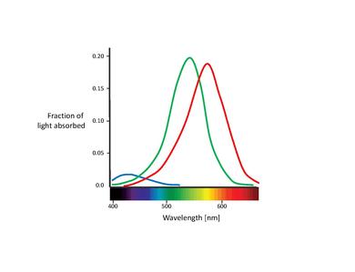
Although no consensus has been reached for naming the different cone types, the most widely utilized designations refer either to their action spectra peak or to the color to which they are sensitive themselves (red, green, blue)[6]. In this text, we will use the S-M-L designation (for short, medium, and long wavelength), since these names are more appropriately descriptive. The blue-green-red nomenclature is somewhat misleading, since all types of cones are sensitive to a large range of wavelengths.
An important feature about the three cone types is their relative distribution in the retina. It turns out that the S-cones present a relatively low concentration through the retina, being completely absent in the most central area of the fovea. Actually, they are too widely spaced to play an important role in spatial vision, although they are capable of mediating weak border perception [12]. The fovea is dominated by L- and M-cones. The proportion of the two latter is usually measured as a ratio. Different values have been reported for the L/M ratio, ranging from 0.67 [13] up to 2 [14], the latter being the most accepted. Why L-cones almost always outnumber the M-cones remains unclear. Surprisingly, the relative cone ratio has almost no significant impact on color vision. This clearly shows that the brain is plastic, capable of making sense out of whatever cone signals it receives [15], [16].
It is also important to note the overlapping of the L- and M-cone absorption spectra. While the S-cone absorption spectrum is clearly separated, the L- and M-cone peaks are only about 30 nm apart, their spectral curves significantly overlapping as well. This results in a high correlation in the photon catches of these two cone classes. This is explained by the fact that in order to achieve the highest possible acuity at the center of the fovea, the visual system treats L- and M-cones equally, not taking into account their absorption spectra. Therefore, any kind of difference leads to a deterioration of the luminance signal [17]. In other words, the small separation between L- and M-cone spectra might be interpreted as a compromise between the needs for high-contrast color vision and high acuity luminance vision. This is congruent with the lack of S-cones in the central part of the fovea, where visual acuity is highest. Furthermore, the close spacing of L- and M-cone absorption spectra might also be explained by their genetic origin. Both cone types are assumed to have evolved "recently" (about 35 million years ago) from a common ancestor, while the S-cones presumably split off from the ancestral receptor much earlier[11].
The spectral absorption functions of the three different types of cone cells are the hallmark of human color vision. This theory solved a long-known problem: although we can see millions of different colors (humans can distinguish between 7 and 10 million different colors[5], our retinas simply do not have enough space to accommodate an individual detector for every color at every retinal location.
From the Retina to the Brain
The signals that are transmitted from the retina to higher levels are not simple point-wise representations of the receptor signals, but rather consist of sophisticated combinations of the receptor signals. The objective of this section is to provide a brief of the paths that some of this information takes.
Once the optical image on the retina is transduced into chemical and electrical signals in the photoreceptors, the amplitude-modulated signals are converted into frequency-modulated representations at the ganglion-cell and higher levels. In these neural cells, the magnitude of the signal is represented in terms of the number of spikes of voltage per second fired by the cell rather than by the voltage difference across the cell membrane. In order to explain and represent the physiological properties of these cells, we will find the concept of receptive fields very useful.
A receptive field is a graphical representation of the area in the visual field to which a given cell responds. Additionally, the nature of the response is typically indicated for various regions in the receptive field. For example, we can consider the receptive field of a photoreceptor as a small circular area representing the size and location of that particular receptor's sensitivity in the visual field. The Figure below shows exemplary receptive fields for ganglion cells, typically in a center-surround antagonism. The left receptive field in the figure illustrates a positive central response (know as on-center). This kind of response is usually generated by a positive input from a single cone surrounded by a negative response generated from several neighboring cones. Therefore, the response of this ganglion cell would be made up of inputs from various cones with both positive and negative signs. In this way, the cell not only responds to points of light, but serves as an edge (or more correctly, a spot) detector. In analogy to the computer vision terminology, we can think of the ganglion cell responses as the output of a convolution with an edge-detector kernel. The right receptive field of in the figure illustrates a negative central response (know as off-center), which is equally likely. Usually, on-center and off-center cells will occur at the same spatial location, fed by the same photoreceptors, resulting in an enhanced dynamic range.
The lower Figure shows that in addition to spatial antagonism, ganglion cells can also have spectral opponency. For instance, the left part of the lower figure illustrates a red-green opponent response with the center fed by positive input from an L-cone and the surrounding fed by a negative input from M-cones. On the other hand, the right part of the lower figure illustrates the off-center version of this cell. Hence, before the visual information has even left the retina, processing has already occurred, with a profound effect on color appearance. There are other types and varieties of ganglion cell responses, but they all share these basic concepts.


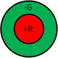

On their way to the primary visual cortex, ganglion cell axons gather to form the optic nerve, which projects to the lateral geniculate nucleus (LGN) in the thalamus. Coding in the optic nerve is highly efficient, keeping the number of nerve fibers to a minimum (limited by the size of the optic nerve) and thereby also the size of the retinal blind spot as small as possible (approximately 5° wide by 7° high). Furthermore, the presented ganglion cells would have no response to uniform illumination, since the positive and negative areas are balanced. In other words, the transmitted signals are uncorrelated. For example, information from neighboring parts of natural scenes are highly correlated spatially and therefore highly predictable [18]. Lateral inhibition between neighboring retinal ganglion cells minimizes this spatial correlation, therefore improving efficiency. We can see this as a process of image compression carried out in the retina.
Given the overlapping of the L- and M-cone absorption spectra, their signals are also highly correlated. In this case, coding efficiency is improved by combining the cone signals in order to minimize said correlation. We can understand this more easily using Principal Component Analysis (PCA). PCA is a statistical method used to reduce the dimensionality of a given set of variables by transforming the original variables, to a set of new variables, the principal components (PCs). The first PC accounts for a maximal amount of total variance in the original variables, the second PC accounts for a maximal amount of variance that was not accounted for by the first component, and so on. In addition, PCs are linearly-independent and orthogonal to each other in the parameter space. PCA's main advantage is that only a few of the strongest PCs are enough to cover the vast majority of system variability [19]. This scheme has been used with the cone absorption functions [20] and even with the naturally occurring spectra[21],[22]. The PCs that were found in the space of cone excitations produced by natural objects are 1) a luminance axis where the L- and M-cone signals are added (L+M), 2) the difference of the L- and M-cone signals (L-M), and 3) a color axis where the S-cone signal is differenced with the sum of the L- and M-cone signals (S-(L+M)). These channels, derived from a mathematical/computational approach, coincide with the three retino-geniculate channels discovered in electrophysiological experiments [23],[24]. Using these mechanisms, visual redundant information is eliminated in the retina.
There are three channels of information that actually communicate this information from the retina through the ganglion cells to the LGN. They are different not only on their chromatic properties, but also in their anatomical substrate. These channels pose important limitations for basic color tasks, such as detection and discrimination.
In the first channel, the output of L- and M-cones is transmitted synergistically to diffuse bipolar cells and then to cells in the magnocellular layers (M-) of the LGN (not to be confused with the M-cones of the retina)[24]. The receptive fields of the M-cells are composed of a center and a surround, which are spatially antagonist. M-cells have high-contrast sensitivity for luminance stimuli, but they show no response at some combination of L-M opponent inputs[25]. However, because the null points of different M-cells vary slightly, the population response is never really zero. This property is actually passed on to cortical areas with predominant M-cell inputs[26].
The parvocellular pathway (P-) originates with the individual outputs from L- or M-cone to midget bipolar cells. These provide input to retinal P-cells[11]. In the fovea, the receptive field centers of P-cells are formed by single L- or M-cones. The structure of the P-cell receptive field surround is still debated. However, the most accepted theory states that the surround consists of a specific cone type, resulting in a spatially opponent receptive field for luminance stimuli[27]. Parvocellular layers contribute with about 80 % of the total projections from the retina to the LGN[28].
Finally, the recently discovered koniocellular pathway (K-) carries mostly signals from S-cones[29]. Groups of this type of cones project to special bipolar cells, which in turn provide input to specific small ganglion cells. These are usually not spatially opponent. The axons of the small ganglion cells project to thin layers of the LGN (adjacent to parvocellular layers)[30].
While the ganglion cells do terminate at the LGN (making synapses with LGN cells), there appears to be a one-to-one correspondence between ganglion cells and LGN cells. The LGN appears to act as a relay station for the signals. However, it probably serves some visual function, since there are neural projections from the cortex back to the LGN that could serve as some type of switching or adaptation feedback mechanism. The axons of LGN cells project to visual area one (V1) in the visual cortex in the occipital lobe.
Color Perception at the Brain
In the cortex, the projections from the magno-, parvo-, and koniocellular pathways end in different layers of the primary visual cortex. The magnocellular fibers innervate principally layer 4Cα and layer 6. Parvocellular neurons project mostly to 4Cβ, and layers 4A and 6. Koniocellular neurons terminate in the cytochrome oxidase (CO-) rich blobs in layers 1, 2, and 3[31].
Once in the visual cortex, the encoding of visual information becomes significantly more complex. In the same way the outputs of various photoreceptors are combined and compared to produce ganglion cell responses, the outputs of various LGN cells are compared and combined to produce cortical responses. As the signals advance further up in the cortical processing chain, this process repeats itself with a rapidly increasing level of complexity to the point that receptive fields begin to lose meaning. However, some functions and processes have been identified and studied in specific regions of the visual cortex.
In the V1 region (striate cortex), double opponent neurons - neurons that have their receptive fields both chromatically and spatially opposite with respect to the on/off regions of a single receptive field - compare color signals across the visual space [32]. They constitute between 5 to 10% of the cells in V1. Their coarse size and small percentage matches the poor spatial resolution of color vision [1]. Furthermore, they are not sensitive to the direction of moving stimuli (unlike some other V1 neurons) and, hence, unlikely to contribute to motion perception[33]. However, given their specialized receptive field structure, these kind of cells are the neural basis for color contrast effects, as well as an efficient mean to encode color itself[34],[35]. Other V1 cells respond to other types of stimuli, such as oriented edges, various spatial and temporal frequencies, particular spatial locations, and combinations of these features, among others. Additionally, we can find cells that linearly combine inputs from LGN cells as well as cells that perform nonlinear combination. These responses are needed to support advanced visual capabilities, such as color itself.

There is substantially less information on the chromatic properties of single neurons in V2 as compared to V1. On a first glance, it seems that there are no major differences of color coding in V1 and V2[36]. One exception to this is the emergence of a new class of color-complex cell[37]. Therefore, it has been suggested that V2 region is involved in the elaboration of hue. However, this is still very controversial and has not been confirmed.
Following the modular concept developed after the discovery of functional ocular dominance in V1, and considering the anatomical segregation between the P-, M-, and K-pathways (described in Sec. 3), it was suggested that a specialized system within the visual cortex devoted to the analysis of color information should exist[38]. V4 is the region that has historically attracted the most attention as the possible "color area" of the brain. This is because of an influential study that claimed that V4 contained 100 % of hue-selective cells[39]. However, this claim has been disputed by a number of subsequent studies, some even reporting that only 16 % of V4 neurons show hue tuning[40]. Currently, the most accepted concept is that V4 contributes not only to color, but to shape perception, visual attention, and stereopsis as well. Furthermore, recent studies have focused on other brain regions trying to find the "color area" of the brain, such as TEO[41] and PITd[42]. The relationship of these regions to each other is still debated. To reconcile the discussion, some use the term posterior inferior temporal (PIT) cortex to denote the region that includes V4, TEO, and PITd[1].
If the cortical response in V1, V2, and V4 cells is already a very complicated task, the level of complexity of complex visual responses in a network of approximately 30 visual zones is humongous. Figure 4 shows a small portion of the connectivity of the different cortical areas (not cells) that have been identified[43].
At this stage, it becomes exceedingly difficult to explain the function of singles cortical cells in simple terms. As a matter of fact, the function of a single cell might not have meaning since the representation of various perceptions must be distributed across collections of cells throughout the cortex.
Color Vision Adaptation Mechanisms
Although researchers have been trying to explain the processing of color signals in the human visual system, it is important to understand that color perception is not a fixed process. Actually, there are a variety of dynamic mechanisms that serve to optimize the visual response according to the viewing environment. Of particular relevance to color perception are the mechanisms of dark, light, and chromatic adaptation.
Dark Adaptation
Dark adaptation refers to the change in visual sensitivity that occurs when the level of illumination is decreased. The visual system response to reduced illumination is to become more sensitive, increasing its capacity to produce a meaningful visual response even when the light conditions are suboptimal[44].
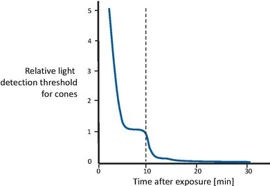
Figure 5 shows the recovery of visual sensitivity after transition from an extremely high illumination level to complete darkness[43]. First, the cones become gradually more sensitive, until the curve levels off after a couple of minutes. Then, after approximately 10 minutes have passed, visual sensitivity is roughly constant. At that point, the rod system, with a longer recovery time, has recovered enough sensitivity to outperform the cones and therefore recover control the overall sensitivity. Rod sensitivity gradually improves as well, until it becomes asymptotic after about 30 minutes. In other words, cones are responsible for the sensitivity recovery for the first 10 minutes. Afterwards, rods outperform the cones and gain full sensitivity after approximately 30 minutes.
This is only one of several neural mechanisms produced in order to adapt to the dark lightning conditions as good as possible. Some other neural mechanisms include the well-known pupil reflex, depletion and regeneration of photopigment, gain control in retinal cells and other higher-level mechanisms, and cognitive interpretation, among others.
Light Adaptation
Light adaptation is essentially the inverse process of dark adaptation. As a matter of fact, the underlying physiological mechanisms are the same for both processes. However, it is important to consider it separately since its visual properties differ.

Light adaptation occurs when the level of illumination is increased. Therefore, the visual system must become less sensitive in order to produce useful perceptions, given the fact that there is significantly more visible light available. The visual system has a limited output dynamic range available for the signals that produce our perceptions. However, the real world has illumination levels covering at least 10 orders of magnitude more. Fortunately, we rarely need to view the entire range of illumination levels at the same time.
At high light levels, adaptation is achieved by photopigment bleaching. This scales photon capture in the receptors and protects the cone response from saturating at bright backgrounds. The mechanisms of light adaptation occur primarily within the retina[45]. As a matter of fact, gain changes are largely cone-specific and adaptation pools signals over areas no larger than the diameter of individual cones[46],[47]. This points to a localization of light adaptation that may be as early as the receptors. However, there appears to be more than one site of sensitivity scaling. Some of the gain changes are extremely rapid, while others take seconds or even minutes to stabilize[48]. Usually, light adaptation takes around 5 minutes (six times faster than dark adaptation). This might point to the influence of post-receptive sites.
Figure 6 shows examples of light adaptation [43]. If we would use a single response function to map the large range of intensities into the visual system's output, then we would only have a very small range at our disposal for a given scene. It is clear that with such a response function, the perceived contrast of any given scene would be limited and visual sensitivity to changes would be severely degraded due to signal-to-noise issues. This case is shown by the dashed line. On the other hand, solid lines represent families of visual responses. These curves map the useful illumination range in any given scene into the full dynamic range of the visual output, thus resulting in the best possible visual perception for each situation. Light adaptation can be thought of as the process of sliding the visual response curve along the illumination level axis until the optimum level for the given viewing conditions is reached.
Chromatic Adaptation
The general concept of chromatic adaptation consists in the variation of the height of the three cone spectral responsivity curves. This adjustment arises because light adaptation occurs independently within each class of cone. A specific formulation of this hypothesis is known as the von Kries adaptation. This hypothesis states that the adaptation response takes place in each of the three cone types separately and is equivalent to multiplying their fixed spectral sensitivities by a scaling constant[49]. If the scaling weights (also known as von Kries coefficients) are inversely proportional to the absorption of light by each cone type (i.e. a lower absorption will require a larger coefficient), then von Kries scaling maintains a constant mean response within each cone class. This provides a simple yet powerful mechanism for maintaining the perceived color of objects despite changes in illumination. Under a number of different conditions, von Kries scaling provides a good account of the effects of light adaptation on color sensitivity and appearance[50],[51].
The easiest way to picture chromatic adaptation is by examining a white object under different types of illumination. For example, let's consider examining a piece of paper under daylight, fluorescent, and incandescent illumination. Daylight contains relatively far more short-wavelength energy than fluorescent light, and incandescent illumination contains relatively far more long-wavelength energy than fluorescent light. However, in spite of the different illumination conditions, the paper approximately retains its white appearance under all three light sources. This is because the S-cone system becomes relatively less sensitive under daylight (in order to compensate for the additional short-wavelength energy) and the L-cone system becomes relatively less sensitive under incandescent illumination (in order to compensate for the additional long-wavelength energy)[43].
References
Auditory System
| This page may need to verify facts by citing reliable publications. You can help by adding references to reliable publications, or by correcting statements cited as fact. |
Introduction
The sensory system for the sense of hearing is the auditory system. This wikibook covers the physiology of the auditory system, and its application to the most successful neurosensory prosthesis - cochlear implants. The physics and engineering of acoustics are covered in a separate wikibook, Acoustics. An excellent source of images and animations is "Journey into the world of hearing" [52].
The ability to hear is not found as widely in the animal kingdom as other senses like touch, taste and smell. It is restricted mainly to vertebrates and insects.[citation needed] Within these, mammals and birds have the most highly developed sense of hearing. The table below shows frequency ranges of humans and some selected animals:[citation needed]
| Humans | 20-20'000 Hz |
|---|---|
| Whales | 20-100'000 Hz |
| Bats | 1'500-100'000 Hz |
| Fish | 20-3'000 Hz |
The organ that detects sound is the ear. It acts as receiver in the process of collecting acoustic information and passing it through the nervous system into the brain. The ear includes structures for both the sense of hearing and the sense of balance. It does not only play an important role as part of the auditory system in order to receive sound but also in the sense of balance and body position.
 |
 |
 |
 |
Humans have a pair of ears placed symmetrically on both sides of the head which makes it possible to localize sound sources. The brain extracts and processes different forms of data in order to localize sound, such as:
- the shape of the sound spectrum at the tympanic membrane (eardrum)
- the difference in sound intensity between the left and the right ear
- the difference in time-of-arrival between the left and the right ear
- the difference in time-of-arrival between reflections of the ear itself (this means in other words: the shape of the pinna (pattern of folds and ridges) captures sound-waves in a way that helps localizing the sound source, especially on the vertical axis.
Healthy, young humans are able to hear sounds over a frequency range from 20 Hz to 20 kHz.[citation needed] We are most sensitive to frequencies between 2000 and 4000 Hz[citation needed] which is the frequency range of spoken words. The frequency resolution is 0.2%[citation needed] which means that one can distinguish between a tone of 1000 Hz and 1002 Hz. A sound at 1 kHz can be detected if it deflects the tympanic membrane (eardrum) by less than 1 Angstrom[citation needed], which is less than the diameter of a hydrogen atom. This extreme sensitivity of the ear may explain why it contains the smallest bone that exists inside a human body: the stapes (stirrup). It is 0.25 to 0.33 cm long and weighs between 1.9 and 4.3 mg.[citation needed]
The following video provides an overview of the concepts that will be presented in more detail in the next sections.
Anatomy of the Auditory System

The aim of this section is to explain the anatomy of the auditory system of humans. The chapter illustrates the composition of auditory organs in the sequence that acoustic information proceeds during sound perception.
Please note that the core information for “Sensory Organ Components” can also be found on the Wikipedia page “Auditory system”, excluding some changes like extensions and specifications made in this article. (see also: Wikipedia Auditory system)
The auditory system senses sound waves, that are changes in air pressure, and converts these changes into electrical signals. These signals can then be processed, analyzed and interpreted by the brain. For the moment, let's focus on the structure and components of the auditory system. The auditory system consists mainly of two parts:
- the ear and
- the auditory nervous system (central auditory system)
The ear
The ear is the organ where the first processing of sound occurs and where the sensory receptors are located. It consists of three parts:
- outer ear
- middle ear
- inner ear

Outer ear
Function: Gathering sound energy and amplification of sound pressure.
The folds of cartilage surrounding the ear canal (external auditory meatus, external acoustic meatus) are called the pinna. It is the visible part of the ear. Sound waves are reflected and attenuated when they hit the pinna, and these changes provide additional information that will help the brain determine the direction from which the sounds came. The sound waves enter the auditory canal, a deceptively simple tube. The ear canal amplifies sounds that are between 3 and 12 kHz. At the far end of the ear canal is the tympanic membrane (eardrum), which marks the beginning of the middle ear.
Middle ear

Function: Transmission of acoustic energy from air to the cochlea.
Sound waves traveling through the ear canal will hit the tympanic membrane (tympanum, eardrum). This wave information travels across the air-filled tympanic cavity (middle ear cavity) via a series of bones: the malleus (hammer), incus (anvil) and stapes (stirrup). These ossicles act as a lever and a teletype, converting the lower-pressure eardrum sound vibrations into higher-pressure sound vibrations at another, smaller membrane called the oval (or elliptical) window, which is one of two openings into the cochlea of the inner ear. The second opening is called round window. It allows the fluid in the cochlea to move.
The malleus articulates with the tympanic membrane via the manubrium, whereas the stapes articulates with the oval window via its footplate. Higher pressure is necessary because the inner ear beyond the oval window contains liquid rather than air. The sound is not amplified uniformly across the ossicular chain. The stapedius reflex of the middle ear muscles helps protect the inner ear from damage.
The middle ear still contains the sound information in wave form; it is converted to nerve impulses in the cochlea.
Inner ear
| Structural diagram of the cochlea | Cross section of the cochlea | Cochlea and Vestibular System from an MRI scan |
|---|---|---|
 |
 |

|
Function: Transformation of mechanical waves (sound) into electric signals (neural signals).
The inner ear consists of the cochlea and several non-auditory structures. The cochlea is a snail-shaped part of the inner ear. It has three fluid-filled sections: scala tympani (lower gallery), scala media (middle gallery, cochlear duct) and scala vestibuli (upper gallery). The cochlea supports a fluid wave driven by pressure across the basilar membrane separating two of the sections (scala tympani and scala media). The basilar membrane is about 3 cm long and between 0.5 to 0.04 mm wide. Reissner’s membrane (vestibular membrane) separates scala media and scala vestibuli.
The scala media contains an extracellular fluid called endolymph, also known as Scarpa's Fluid after Antonio Scarpa. The organ of Corti is located in this duct, and transforms mechanical waves to electric signals in neurons. The other two sections, scala tympani and scala vestibuli, are located within the bony labyrinth which is filled with fluid called perilymph. The chemical difference between the two fluids endolymph (in scala media) and perilymph (in scala tympani and scala vestibuli) is important for the function of the inner ear.
Organ of Corti
The organ of Corti forms a ribbon of sensory epithelium which runs lengthwise down the entire cochlea. The hair cells of the organ of Corti transform the fluid waves into nerve signals. The journey of a billion nerves begins with this first step; from here further processing leads to a series of auditory reactions and sensations.
Transition from ear to auditory nervous system

Hair cells
Hair cells are columnar cells, each with a bundle of 100-200 specialized cilia at the top, for which they are named. These cilia are the mechanosensors for hearing. The shorter ones are called stereocilia, and the longest one at the end of each haircell bundle kinocilium. The location of the kinocilium determine the on-direction, i.e. the direction of deflection inducing the maximum hair cell excitation. Lightly resting atop the longest cilia is the tectorial membrane, which moves back and forth with each cycle of sound, tilting the cilia and allowing electric current into the hair cell.
The function of hair cells is not fully established up to now. Currently, the knowledge of the function of hair cells allows to replace the cells by cochlear implants in case of hearing lost. However, more research into the function of the hair cells may someday even make it possible for the cells to be repaired. The current model is that cilia are attached to one another by “tip links”, structures which link the tips of one cilium to another. Stretching and compressing, the tip links then open an ion channel and produce the receptor potential in the hair cell. Note that a deflection of 100 nanometers already elicits 90% of the full receptor potential.
Neurons
The nervous system distinguishes between nerve fibres carrying information towards the central nervous system and nerve fibres carrying the information away from it:
- Afferent neurons (also sensory or receptor neurons) carry nerve impulses from receptors (sense organs) towards the central nervous system
- Efferent neurons (also motor or effector neurons) carry nerve impulses away from the central nervous system to effectors such as muscles or glands (and also the ciliated cells of the inner ear)
Afferent neurons innervate cochlear inner hair cells, at synapses where the neurotransmitter glutamate communicates signals from the hair cells to the dendrites of the primary auditory neurons.
There are far fewer inner hair cells in the cochlea than afferent nerve fibers. The neural dendrites belong to neurons of the auditory nerve, which in turn joins the vestibular nerve to form the vestibulocochlear nerve, or cranial nerve number VIII'
Efferent projections from the brain to the cochlea also play a role in the perception of sound. Efferent synapses occur on outer hair cells and on afferent (towards the brain) dendrites under inner hair cells.
Auditory nervous system
The sound information, now re-encoded in form of electric signals, travels down the auditory nerve (acoustic nerve, vestibulocochlear nerve, VIIIth cranial nerve), through intermediate stations such as the cochlear nuclei and superior olivary complex of the brainstem and the inferior colliculus of the midbrain, being further processed at each waypoint. The information eventually reaches the thalamus, and from there it is relayed to the cortex. In the human brain, the primary auditory cortex is located in the temporal lobe.
Primary auditory cortex
The primary auditory cortex is the first region of cerebral cortex to receive auditory input.
Perception of sound is associated with the right posterior superior temporal gyrus (STG). The superior temporal gyrus contains several important structures of the brain, including Brodmann areas 41 and 42, marking the location of the primary auditory cortex, the cortical region responsible for the sensation of basic characteristics of sound such as pitch and rhythm.
The auditory association area is located within the temporal lobe of the brain, in an area called the Wernicke's area, or area 22. This area, near the lateral cerebral sulcus, is an important region for the processing of acoustic signals so that they can be distinguished as speech, music, or noise.
Auditory Signal Processing
Now that the anatomy of the auditory system has been sketched out, this topic goes deeper into the physiological processes which take place while perceiving acoustic information and converting this information into data that can be handled by the brain. Hearing starts with pressure waves hitting the auditory canal and is finally perceived by the brain. This section details the process transforming vibrations into perception.
Effect of the head
Sound waves with a wavelength shorter than the head produce a sound shadow on the ear further away from the sound source. When the wavelength is longer than the head, diffraction of the sound leads to approximately equal sound intensities on both ears.

Sound reception at the pinna
The pinna collects sound waves in air affecting sound coming from behind and the front differently with its corrugated shape. The sound waves are reflected and attenuated or amplified. These changes will later help sound localization.
In the external auditory canal, sounds between 3 and 12 kHz - a range crucial for human communication - are amplified. It acts as resonator amplifying the incoming frequencies.
Sound conduction to the cochlea
Sound that entered the pinna in form of waves travels along the auditory canal until it reaches the beginning of the middle ear marked by the tympanic membrane (eardrum). Since the inner ear is filled with fluid, the middle ear is kind of an impedance matching device in order to solve the problem of sound energy reflection on the transition from air to the fluid. As an example, on the transition from air to water 99.9% of the incoming sound energy is reflected. This can be calculated using:

with Ir the intensity of the reflected sound, Ii the intensity of the incoming sound and Zk the wave resistance of the two media ( Zair = 414 kg m-2 s-1 and Zwater = 1.48*106 kg m-2 s-1). Three factors that contribute the impedance matching are:
- the relative size difference between tympanum and oval window
- the lever effect of the middle ear ossicles and
- the shape of the tympanum.

The longitudinal changes in air pressure of the sound-wave cause the tympanic membrane to vibrate which, in turn, makes the three chained ossicles malleus, incus and stirrup oscillate synchronously. These bones vibrate as a unit, elevating the energy from the tympanic membrane to the oval window. In addition, the energy of sound is further enhanced by the areal difference between the membrane and the stapes footplate. The middle ear acts as an impedance transformer by changing the sound energy collected by the tympanic membrane into greater force and less excursion. This mechanism facilitates transmission of sound-waves in air into vibrations of the fluid in the cochlea. The transformation results from the pistonlike in- and out-motion by the footplate of the stapes which is located in the oval window. This movement performed by the footplate sets the fluid in the cochlea into motion.
Through the stapedius muscle, the smallest muscle in the human body, the middle ear has a gating function: contracting this muscle changes the impedance of the middle ear, thus protecting the inner ear from damage through loud sounds.
Frequency analysis in the cochlea
The three fluid-filled compartements of the cochlea (scala vestibuli, scala media, scala tympani) are separated by the basilar membrane and the Reissner’s membrane. The function of the cochlea is to separate sounds according to their spectrum and transform it into a neural code.
When the footplate of the stapes pushes into the perilymph of the scala vestibuli, as a consequence the membrane of Reissner bends into the scala media. This elongation of Reissner’s membrane causes the endolymph to move within the scala media and induces a displacement of the basilar membrane.
The separation of the sound frequencies in the cochlea is due to the special properties of the basilar membrane. The fluid in the cochlea vibrates (due to in- and out-motion of the stapes footplate) setting the membrane in motion like a traveling wave. The wave starts at the base and progresses towards the apex of the cochlea. The transversal waves in the basilar membrane propagate with

with μ the shear modulus and ρ the density of the material. Since width and tension of the basilar membrane change, the speed of the waves propagating along the membrane changes from about 100 m/s near the oval window to 10 m/s near the apex.
There is a point along the basilar membrane where the amplitude of the wave decreases abruptly. At this point, the sound wave in the cochlear fluid produces the maximal displacement (peak amplitude) of the basilar membrane. The distance the wave travels before getting to that characteristic point depends on the frequency of the incoming sound. Therefore each point of the basilar membrane corresponds to a specific value of the stimulating frequency. A low-frequency sound travels a longer distance than a high-frequency sound before it reaches its characteristic point. Frequencies are scaled along the basilar membrane with high frequencies at the base and low frequencies at the apex of the cochlea.

Identifying frequency by the location of the maximum displacement of the basilar membrane is called tonotopic encoding of frequency. It automatically solves two problems:
- It automatically parallelizes the subsequent processing of frequency. This tonotopic encoding is maintained all the way up to the cortex.
- Our nervous system transmits information with action potentials, which are limited to less than 500 Hz. Through tonotopic encoding, also higher frequencies can be accurately represented.
Sensory transduction in the cochlea
Most everyday sounds are composed of multiple frequencies. The brain processes the distinct frequencies, not the complete sounds. Due to its inhomogeneous properties, the basilar membrane is performing an approximation to a Fourier transform. The sound is thereby split into its different frequencies, and each hair cell on the membrane corresponds to a certain frequency. The loudness of the frequencies is encoded by the firing rate of the corresponding afferent fiber. This is due to the amplitude of the traveling wave on the basilar membrane, which depends on the loudness of the incoming sound.


The sensory cells of the auditory system, known as hair cells, are located along the basilar membrane within the organ of Corti. Each organ of Corti contains about 16,000 such cells, innervated by about 30,000 afferent nerve fibers. There are two anatomically and functionally distinct types of hair cells: the inner and the outer hair cells. Along the basilar membrane these two types are arranged in one row of inner cells and three to five rows of outer cells. Most of the afferent innervation comes from the inner hair cells while most of the efferent innervation goes to the outer hair cells. The inner hair cells influence the discharge rate of the individual auditory nerve fibers that connect to these hair cells. Therefore inner hair cells transfer sound information to higher auditory nervous centers. The outer hair cells, in contrast, amplify the movement of the basilar membrane by injecting energy into the motion of the membrane and reducing frictional losses but do not contribute in transmitting sound information. The motion of the basilar membrane deflects the stereocilias (hairs on the hair cells) and causes the intracellular potentials of the hair cells to decrease (depolarization) or increase (hyperpolarization), depending on the direction of the deflection. When the stereocilias are in a resting position, there is a steady state current flowing through the channels of the cells. The movement of the stereocilias therefore modulates the current flow around that steady state current.
Let's look at the modes of action of the two different hair cell types separately:
- Inner hair cells:
The deflection of the hair-cell stereocilia opens mechanically gated ion channels that allow small, positively charged potassium ions (K+) to enter the cell and causing it to depolarize. Unlike many other electrically active cells, the hair cell itself does not fire an action potential. Instead, the influx of positive ions from the endolymph in scala media depolarizes the cell, resulting in a receptor potential. This receptor potential opens voltage gated calcium channels; calcium ions (Ca2+) then enter the cell and trigger the release of neurotransmitters at the basal end of the cell. The neurotransmitters diffuse across the narrow space between the hair cell and a nerve terminal, where they then bind to receptors and thus trigger action potentials in the nerve. In this way, neurotransmitter increases the firing rate in the VIIIth cranial nerve and the mechanical sound signal is converted into an electrical nerve signal.
The repolarization in the hair cell is done in a special manner. The perilymph in Scala tympani has a very low concentration of positive ions. The electrochemical gradient makes the positive ions flow through channels to the perilymph. (see also: Wikipedia Hair cell)
- Outer hair cells:
In humans' outer hair cells, the receptor potential triggers active vibrations of the cell body. This mechanical response to electrical signals is termed somatic electromotility and drives oscillations in the cell’s length, which occur at the frequency of the incoming sound and provide mechanical feedback amplification. Outer hair cells have evolved only in mammals. Without functioning outer hair cells the sensitivity decreases by approximately 50 dB (due to greater frictional losses in the basilar membrane which would damp the motion of the membrane). They have also improved frequency selectivity (frequency discrimination), which is of particular benefit for humans, because it enables sophisticated speech and music. (see also: Wikipedia Hair cell)
With no external stimulation, auditory nerve fibres discharge action potentials in a random time sequence. This random time firing is called spontaneous activity. The spontaneous discharge rates of the fibers vary from very slow rates to rates of up to 100 per second. Fibers are placed into three groups depending on whether they fire spontaneously at high, medium or low rates. Fibers with high spontaneous rates (> 18 per second) tend to be more sensitive to sound stimulation than other fibers.
Auditory pathway of nerve impulses

So in the inner hair cells the mechanical sound signal is finally converted into electrical nerve signals. The inner hair cells are connected to auditory nerve fibres whose nuclei form the spiral ganglion. In the spiral ganglion the electrical signals (electrical spikes, action potentials) are generated and transmitted along the cochlear branch of the auditory nerve (VIIIth cranial nerve) to the cochlear nucleus in the brainstem.
From there, the auditory information is divided into at least two streams:
- Ventral Cochlear Nucleus:
One stream is the ventral cochlear nucleus which is split further into the posteroventral cochlear nucleus (PVCN) and the anteroventral cochlear nucleus (AVCN). The ventral cochlear nucleus cells project to a collection of nuclei called the superior olivary complex.
Superior olivary complex: Sound localization
The superior olivary complex - a small mass of gray substance - is believed to be involved in the localization of sounds in the azimuthal plane (i.e. their degree to the left or the right). There are two major cues to sound localization: Interaural level differences (ILD) and interaural time differences (ITD). The ILD measures differences in sound intensity between the ears. This works for high frequencies (over 1.6 kHz), where the wavelength is shorter than the distance between the ears, causing a head shadow - which means that high frequency sounds hit the averted ear with lower intensity. Lower frequency sounds don't cast a shadow, since they wrap around the head. However, due to the wavelength being larger than the distance between the ears, there is a phase difference between the sound waves entering the ears - the timing difference measured by the ITD. This works very precisely for frequencies below 800 Hz, where the ear distance is smaller than half of the wavelength. Sound localization in the median plane (front, above, back, below) is helped through the outer ear, which forms direction-selective filters.
There, the differences in time and loudness of the sound information in each ear are compared. Differences in sound intensity are processed in cells of the lateral superior olivary complexm and timing differences (runtime delays) in the medial superior olivary complex. Humans can detect timing differences between the left and right ear down to 10 μs, corresponding to a difference in sound location of about 1 deg. This comparison of sound information from both ears allows the determination of the direction where the sound came from. The superior olive is the first node where signals from both ears come together and can be compared. As a next step, the superior olivary complex sends information up to the inferior colliculus via a tract of axons called lateral lemniscus. The function of the inferior colliculus is to integrate information before sending it to the thalamus and the auditory cortex. It is interesting to know that the superior colliculus close by shows an interaction of auditory and visual stimuli.
- Dorsal Cochlear Nucleus:
The dorsal cochlear nucleus (DCN) analyzes the quality of sound and projects directly via the lateral lemnisucs to the inferior colliculus.
From the inferior colliculus the auditory information from ventral as well as dorsal cochlear nucleus proceeds to the auditory nucleus of the thalamus which is the medial geniculate nucleus. The medial geniculate nucleus further transfers information to the primary auditory cortex, the region of the human brain that is responsible for processing of auditory information, located on the temporal lobe. The primary auditory cortex is the first relay involved in the conscious perception of sound.
Primary auditory cortex and higher order auditory areas
Sound information that reaches the primary auditory cortex (Brodmann areas 41 and 42). The primary auditory cortex is the first relay involved in the conscious perception of sound. It is known to be tonotopically organized and performs the basics of hearing: pitch and volume. Depending on the nature of the sound (speech, music, noise), is further passed to higher order auditory areas. Sounds that are words are processed by Wernicke’s area (Brodmann area 22). This area is involved in understanding written and spoken language (verbal understanding). The production of sound (verbal expression) is linked to Broca’s area (Brodmann areas 44 and 45). The muscles to produce the required sound when speaking are contracted by the facial area of motor cortex which are regions of the cerebral cortex that are involved in planning, controlling and executing voluntary motor functions.

Pitch Perception
This section reviews a key topic in auditory neuroscience: pitch perception. Some basic understanding of the auditory system is presumed, so readers are encouraged to first read the above sections on the 'Anatomy of the Auditory System' and 'Auditory Signal Processing'.
Introduction
Pitch is a subjective percept, evoked by sounds that have an approximately periodic nature. For many naturally occurring sounds, periodicity of a sound is the major determinant of pitch. Yet the relationship between an acoustic stimulus and pitch is quite abstract: in particular, pitch is quite robust to changes in other acoustic parameters such as loudness or spectral timbre, both of which may significantly alter the physical properties of an acoustic waveform. This is particularly evident in cases where sounds without any shared spectral components can evoke the same pitch, for example. Consequently, pitch-related information must be extracted from spectral and/or temporal cues represented across multiple frequency channels.
Investigations of pitch encoding in the auditory system have largely focused on identifying neural processes which reflect these extraction processes, or on finding the ‘end point’ of such a process: an explicit, robust representation of pitch as perceived by the listener. Both endeavours have had some success, with evidence accumulating for ‘pitch selective neurons’ in putative ‘pitch areas’. However, it remains debatable whether the activity of these areas is truly related to pitch, or if they simply exhibit selective representation of pitch-related parameters. On the one hand, demonstrating an activation of specific neurons or neural areas in response to numerous pitch-evoking sounds, often with substantial variation in their physical characteristics, provides compelling correlative evidence that these regions are indeed encoding pitch. On the other, demonstrating causal evidence that these neurons represent pitch is difficult, likely requiring a combination of in vivo recording approaches to demonstrate a correspondence of these responses to pitch judgments (i.e., psychophysical responses, rather than just stimulus periodicity), and direct manipulation of the activity in these cells to demonstrate predictable biases or impairments in pitch perception.
Due to the rather abstract nature of pitch, we will not immediately delve into this yet unresolved field of active research. Rather, we begin our discussion with the most direct physical counterparts of pitch perception – i.e., sound frequency (for pure tones) and, more generally, stimulus periodicity. Specifically, we will distinguish between, and more concretely define, the notions of periodicity and pitch. Following this, we will briefly outline the major computational mechanisms that may be implemented by the auditory system to extract such pitch-related information from sound stimuli. Subsequently, we outline representation and processing of pitch parameters in the cochlea, the ascending subcortical auditory pathway, and, finally, more controversial findings in primary auditory cortex and beyond, and evaluate the evidence of ‘pitch neurons’ or ‘pitch areas’ in these cortical regions.
Periodicity and pitch
Pitch is an emergent psychophysical property. The salience and ‘height’ of pitch depends on several factors, but within a specific range of harmonic and fundamental frequencies, called the “existence region”, pitch salience is largely determined by regularity of sound segment repetition; pitch height by the rate of repetition, also called the modulating frequency. The set of sounds capable of evoking pitch perception is diverse and spectrally heterogeneous. Many different stimuli – including pure tones, click trains, iterated ripple noises, amplitude modulated sounds, and so forth – can evoke a pitch percept, while another acoustic signals, even with very similar physical characteristics to such stimuli may not evoke pitch. Most naturally occurring pitch-evoking sounds are harmonic complexes - sounds containing a spectrum of frequencies that are integer multiples of the fundamental frequency, F0. An important finding in pitch research is the phenomenon of the ‘missing fundamental’ (see below): within a certain frequency range, all the spectral energy at F0 can be removed from a harmonic complex, and still evoke a pitch correlating to F0 in a human listener[53]. This finding appears to generalise to many non-human auditory systems[54][55].

| Demo: Pitch of the missing fundamental
Melody played with only harmonic overtones, with spectral energy at the fundamental frequencies removed. fhead
|
|
| Problems listening to these files? See media help. | |
The ‘missing fundamental’ phenomenon is important for two reasons. Firstly, it is an important benchmark for assessing whether particular neurons or brain regions are specialised for pitch processing, since such units should be expected to show activity reflective of F0 (and thus pitch), regardless of its presence in the sound and other acoustic parameters. More generally, a ‘pitch neuron’ or ‘pitch centre’ should show consistent activity in response to all stimuli that evoke a particular perception of pitch height. As will be discussed, this has been a source of some disagreement in identifying putative pitch neurons or areas. Secondly, that we can perceive a pitch corresponding to F0 even in its absence in the auditory stimulus provides strong evidence against the brain implementing a mechanism for ‘selecting’ F0 to directly infer pitch. Rather, pitch must be extracted from temporal or spectral cues (or both)[56].
Mechanisms for pitch extraction: spectral and temporal cues

These two cues (spectral and temporal) are the bases of two major classes of pitch extraction models[56]. The first of these are the time domain methods, which use temporal cues to assess whether a sound consists of a repetitive segment, and, if so, the rate of repetition. A commonly proposed method of doing so is autocorrelation. An autocorrelation function essentially involves finding the time delays between two sampling points that will give the maximum correlation: for example, a sound wave with a frequency of 100Hz (or period, T=10 milliseconds) would have a maximal correlation if samples are taken 10 milliseconds apart. For a 200Hz wave, the delay yielding maximal correlation would be 5 milliseconds – but also at 10 milliseconds, 15 milliseconds and so forth. Thus if such a function is performed on all component frequencies of a harmonic complex with F0=100Hz (and thus having harmonic overtones at 200Hz, 300Hz, 400Hz, and so forth), and the resulting time intervals giving maximal correlation were summed, they would collectively ‘vote’ for 10 milliseconds – the periodicity of the sound. The second class of pitch extraction strategies are frequency domain methods, where pitch is extracted by analysing the frequency spectra of a sound to calculate F0. For instance, ‘template matching' processes – such as the ‘harmonic sieve’ – propose that the frequency spectrum of a sound is simply matched to harmonic templates – the best match yields the correct F0[57].
There are limitations to both classes of explanations. Frequency domain methods require harmonic frequencies to be resolved – that is, for each harmonic to be represented as a distinct frequency band (see figure, right). Yet higher order harmonics, which are unresolved due to the wider bandwidth in physiological representation for higher frequencies (a consequence of the logarithmic tonotopic organisation of the basilar membrane), can still evoke pitch corresponding to F0. Temporal models do not have this issue, since an autocorrelation function should still yield the same periodicity, regardless of whether the function is performed in one or over several frequency channels. However, it is difficult to attribute the lower limits of pitch-evoking frequencies to autocorrelation: psychophysical studies demonstrate that we can perceive pitch from harmonic complexes with missing fundamentals as low as 30Hz; this corresponds to a sampling delay of over 33 milliseconds – far longer than the ~10 millisecond delay commonly observed in neural signalling[56].

One strategy to determine which of these two strategies are adopted by the auditory system is the use of alternating-phase harmonics: to present odd harmonics in sine phase, and even harmonics in cosine phase. Since this will not affect the spectral content of the stimulus, no change in pitch perception should occur if the listener is relying primarily on spectral cues. On the other hand, the temporal envelope repetition rate will double. Thus, if temporal envelope cues are adopted, the pitch perceived by listeners for alternating-phase harmonics will be an octave above (i.e., double the frequency of) the pitch perceived for all-cosine harmonic with the same spectral composition. Psychophysical studies have investigated the sensitivity of pitch perception to such phase shifts across different F0 and harmonic ranges, providing evidence that both humans[58] and other primates[59] adopt a dual strategy: spectral cues are used for lower order, resolved harmonics, while temporal envelope cues are used higher order, unresolved harmonics.
Pitch extraction in the ascending auditory pathway
Weber fractions for pitch discrimination in humans has been reported at under 1%[60]. In view of this high sensitivity to pitch changes, and the demonstration that both spectral and temporal cues are used for pitch extraction, we can predict that the auditory system represents both the spectral composition and temporal fine structure of acoustic stimuli in a highly precise manner, until these representations are eventually conveyed explicitly periodicity or pitch-selective neurons.
Electrophysiological experiments have identified neuronal responses in the ascending auditory system that are consistent with this notion. From the level of the cochlea, the tonopically mapped basilar membrane’s (BM) motions in response to auditory stimuli establishes a place code for frequency composition along the BM axis. These representations are further enhanced by a phase-locking of the auditory nerve fibres (ANFs) to the frequency components it responds to. This mechanism for temporal representation of frequency composition is further enhanced in numerous ways, such as lateral inhibition at the hair cell/spiral ganglion cell synapse[61], supporting the notion that this precise representation is critical for pitch encoding.
Thus by this stage, the phase-locked temporal spike patterns of ANFs likely carry an implicit representation of periodicity. This was tested directly by Cariani and Delgutte[62]. By analysing the distribution of all-order inter-spike intervals (ISI) in the ANFs of cats, they showed that the most common ISI was the periodicity of the stimulus, and the peak-to-mean ratio of these distribution increased for complex stimuli evoking more salient pitch perceptions. Based on these findings, these authors proposed the ‘predominant interval hypothesis’, where a pooled code of all-order ISIs ‘vote’ for the periodicity - though of course, this finding is an inevitable consequence of phase-locked responses of ANFs. In addition, there is evidence that the place code for frequency components is also critical. By crossing a low-frequency stimulus with a high-frequency carrier, Oxenham et al transposed the temporal fine-structure of the low frequency sinusoid to higher frequency regions along the BM.[63] This led to significantly impaired pitch discrimination abilities. Thus, both the place and temporal coding represent pitch-related information in the ANFs.
The auditory nerve carries information to the cochlear nucleus (CN). Here, many cell types represent pitch-related information in different ways. For example, many bushy cells appear to have little difference in firing properties of auditory nerve fibres – information may be carried to higher order brain regions without significant modification[56].Of particular interest are the sustained chopper cells in the ventral cochlear nucleus. According Winter and colleagues, the first-order spike intervals in these cells corresponds to periodicity in response to iterated rippled noise stimuli (IRN), as well to cosine-phase and random-phase harmonic complexes, quite invariantly to sound level[64]. While further characterisation of these cells' responses to different pitch-evoking stimuli is required, there is therefore some indication that pitch extraction may begin as early as the level of the CN.
In the inferior colliculus (IC), there is some evidence that the average response rate of neurons is equal to the periodicity of the stimulus[65]. Subsequent studies comparing IC neuron responses to same-phase and alternating-phase harmonic complexes suggest that these cells may be responding to the periodicity of the overall energy level (i.e., the envelope), rather than true modulating frequency, yet it is not clear whether this applies only for unresolved harmonics (as would be predicted by psychophysical experiments) or also for resolved harmonics[56]. There remains much uncertainty regarding the representation of periodicity in the IC.
Pitch coding in the auditory cortex
Thus, there is a tendency to enhance that representations of F0 throughout the ascending auditory system, though the precise nature of this remains unclear. In these subcortical stages of the ascending auditory pathway however, there is no evidence for an explicit representation that consistently encodes information corresponding to perceived pitch. Such representations likely occur in ‘higher’ auditory regions, from primary auditory cortex onward.
Indeed, lesion studies have demonstrated the necessity for auditory cortex in pitch perception. Of course, an impairment in pitch detection following lesions to the auditory cortex may simply be reflect a passive transmission role for the cortex: where subcortical information must ‘pass through’ to affect behaviour. Yet studies such as that by Whitfield have demonstrated that this is likely not the case: while decorticate cats could be re-trained (following an ablation of their auditory cortex) to recognise complex tones comprised of three frequency components, the animals selectively lost the ability generalise these tones to other complexes with the same pitch[66]. In other words, while the harmonic composition could influence behaviour, harmonic relations (i.e. a pitch cue) could not. For example, the lesioned animal could correctly respond to a pure tone at 100Hz, but would not respond to a harmonic complex consisting of its harmonic overtones (at 200Hz, 300Hz, and so forth). This suggests strongly a role for the auditory cortex in further extraction of pitch-related information.
Early MEG studies of the primary auditory cortex had suggested that A1 contained a map of pitch. This was based on the findings that a pure tone and its missing fundamental harmonic complex (MF) evoked stimulus-evoked excitation (called the N100m) in the same location, whereas components frequencies of the MF presented in isolation evoked excitations in different locations[67]. Yet such notions were overcast by the results of experiments using higher spatial-resolution techniques: local field potential (LFP) and multi-unit recording (MUA) demonstrated that the mapping A1 was tonotopic – that is, based on neurons’ best frequency (BF), rather than best ‘pitch’[68]. These techniques do however demonstrate an emergence of distinct coding mechanisms reflective of extracting temporal and spectral cues: phase-locked representation of temporal envelope repetition rate was recorded in the higher BF regions of the tonotopic map, while the harmonic structure of the click train was represented in lower BF regions[69].Thus, the cues for pitch extraction may be further enhanced by this stage.

An example of a neuronal substrate that may facilitate such an enhancement was described by Kadia and Wang in primary auditory cortex of marmosets[70]. Around 20% of the neurons here could be classified as ‘multi-peaked’ units: neurons that have multiple frequency response areas, often in harmonic relation (see figure, right). Further, excitation of two of these spectral peaks what shown to have a synergistic effect on the neurons’ responses. This would therefore facilitate the extraction of harmonically related tones in the acoustic stimulus, allowing these neurons to act as a ‘harmonic template’ for extracting spectral cues. Additionally, these authors observed that in the majority of ‘single peaked’ neurons (i.e. neurons with a single spectral tuning peak at its BF), a secondary tone could have a modulatory (facilitating or inhibiting) effect on the response of the neuron to its BF. Again, these modulating frequencies were often harmonically related to the BF. These facilitating mechanisms may therefore accommodate the extraction of certain harmonic components, while rejecting other spectral combinations through inhibitory modulation may facilitate the disambiguation with other harmonic complexes or non-harmonic complexes such as broadband noise.

However, given that the tendency to enhance F0 has been demonstrated throughout the subcortical auditory system, we might expect have to come closer to a more explicit representation of pitch in the cortex. Neuroimaging experiments have explored this idea, capitalising on the emergent quality of pitch: a subtractive method can identify areas in the brain which show BOLD responses in response to a pitch-evoking stimulus, but not to another sound with very similar spectral properties, but does not evoke pitch perception. Such strategies were used by Patterson, Griffiths and colleagues: by subtracting the BOLD signal acquired during presentation of broad-band noise from the signal acquired during presentation of IRN, they identified a selective activation of the lateral (and to some extent, medial) Heschl’s gyrus (HG) in response to the latter class of pitch-evoking sounds[71]. Further, varying the repetition rate of IRN over time to create a melody led to additional activation in the superior temporal gyrus (STG) and planum polare (PP), suggesting a hierarchical processing of pitch through the auditory cortex. In line with this, MEG recordings by Krumbholz et al showed that, as the repetition rate of IRN stimuli is increased, a novel N100m is detected around the HG as the repetition rate crosses the lower threshold for pitch perception, and the magnitude of this “pitch-onset response” increased with pitch salience[72].
There is however some debate about the precise location of the pitch selective area. As Hall and Plack point out, the use of IRN stimuli alone to identify pitch-sensitive cortical areas is insufficient to capture the broad range of stimuli that can induce pitch perception: the activation of HG may be specific to repetitive broadband stimuli[73]. Indeed, based on BOLD signals observed in response to multiple pitch-evoking stimuli, Hall and Plack suggest that the planum temporale (PT) is more relevant for pitch processing.
Despite ongoing disagreement about the precise neural area specialised for pitch coding, such evidence suggests that regions lying anterolateral to A1 may be specialised for pitch perception. Further support for this notion is provided by the identification of ‘pitch selective’ neurons at the anterolateral border of A1 in the marmoset auditory cortex. These neurons were selectively responsive to both pure tones and missing F0 harmonics with the similar periodicities[74]. Many of these neurons were also sensitive to the periodicity of other pitch-evoking stimuli, such as click trains or IRN noise. This provides strong evidence that these neurons are not merely responding any particular component of the acoustic signal, but specifically represent pitch-related information.
Periodicity coding or pitch coding?
Accumulating evidence thus suggests that there are neurons and neural areas specialised in extracting F0, likely in regions just anterolateral to the low BF regions of A1. However, there are still difficulties in calling these neurons or areas “pitch selective”. While stimulus F0 is certainly a key determinant of pitch, it is not necessarily equivalent to the pitch perceived by the listener.
There are however several lines of evidence suggesting that these regions are indeed coding pitch, rather than just F0. For instance, further investigation of the marmoset pitch-selective units by Bendor and colleagues has demonstrated that the activity in these neurons corresponds well to the animals' psychophysical responses[59]. These authors tested the animals’ abilities to detect an alternating-phase harmonic complex amidst an ongoing presentation of same-phase harmonics at the same F0, in order to distinguish between when animals rely more on temporal envelope cues for pitch perception, rather than spectral cues. Consistent with psychophysical experiments in humans, the marmosets used primarily temporal envelope cues for higher order, unresolved harmonics of low F0, while spectral cues were used to extract pitch from lower-order harmonics of high F0 complexes. Recording from these pitch selective neurons showed that the F0 tuning shifted down an octave for alternating-phase harmonics, compared to same-phase harmonics for neurons tuned to low F0s. These patterns of neuronal responses are thus consistent with the psychophysical results, and suggest that both temporal and spectral cues are integrated in these neurons to influence pitch perception.
Yet, again, this study cannot definitively distinguish whether these pitch-selective neurons explicitly represent pitch, or simply an integration of F0 information that will then be subsequently decoded to perceive pitch. A more direct approach to addressing this issue was taken by Bizley et al, who analysed how auditory cortex LFP and MUA measurements in ferrets could independently be used to estimate stimulus F0 and pitch perception[75]. While ferrets were engaged in a pitch discrimination task (to indicate whether a target artificial vowel sound was higher or lower in pitch than a reference in a 2-alternative forced choice paradigm), receiver operating characteristic (ROC) analysis was used to estimate the discriminability of neural activity in predicting the change in F0 or the actual behavioural choice (i.e. a surrogate for perceived pitch). They found that neural responses across the auditory cortex were informative regarding both. Initially, the activity better discriminated F0 than the animal’s choice, but information regarding the animals’ choice grew steadily higher throughout the post-stimulus interval, eventually becoming more discriminable than the direction of F0 change[75].
Comparing the differences in ROC between the cortical areas studied showed that posterior fields activity better discriminated the ferrets’ choice. This may be interpreted in two ways. Since choice-related activity was higher in the posterior fields (which lie by the low BF border of A1), compared to the primary fields, this may be seen as further evidence for pitch-selectivity near low BF border of A1. On the other hand, the fact the pitch-related information was also observed in the primary auditory fields may suggest that sufficient pitch-related information may already be established by this stage, or that a distributed code across multiple auditory areas code pitch. Indeed, while single neurons distributed across the auditory cortex are in general sensitive to multiple acoustic parameters (and therefore not ‘pitch-selective’), information theoretic or neurometric analyses (using neural data to infer stimulus-related information) indicate that pitch information can nevertheless be robustly represented via population coding, or even by single neurons through temporal multiplexing (i.e., representing multiple sound features in distinct time windows)[76][77]. Thus, in the absence of stimulation or deactivation of these putative pitch-selective neurons or areas to demonstrate that such interventions induce predictable biases or impairments in pitch, it may be that pitch is represented in spatially and temporally distributed codes across the auditory cortex, rather than relying on specialised local representations.
Thus, both electrophysiological recording and neuroimaging studies suggest that there may be an explicit neural code for pitch lies near the low BF border of A1. Certainly, the consistent and selective responses to a wide range of pitch-evoking stimuli suggest that these putative pitch-selective neurons and areas are not simply reflecting any immediately available physical characteristic of the acoustic signal. Moreover, there is evidence that these putative pitch-selective neurons extract information from spectral and temporal cues in much the same way as the animal. However, by virtue of the abstract relationship between pitch and an acoustic signal, such correlative evidence between a stimulus and neural response can only be interpreted as evidence that the auditory system has the capacity to form enhanced representations of pitch-related parameters. Without more direct causal evidence for these putative pitch-selective neurons and neural areas determining pitch perception, we cannot conclude whether animals do indeed rely on such localised explicit codes for pitch, or if the robust distributed representations of pitch across the auditory cortex mark the final coding of pitch in the auditory system.
References
- ↑ a b c d Conway, Bevil R (2009). "Color vision, cones, and color-coding in the cortex". The neuroscientist. 15: 274–290.
- ↑ Russell, Richard and Sinha, Pawan} (2007). "Real-world face recognition: The importance of surface reflectance properties". Perception. 36 (9).
{{cite journal}}: CS1 maint: multiple names: authors list (link) - ↑ Gegenfurtner, Karl R and Rieger, Jochem (2000). "Sensory and cognitive contributions of color to the recognition of natural scenes". Current Biology. 10 (13): 805–808.
{{cite journal}}: CS1 maint: multiple names: authors list (link) - ↑ Changizi, Mark A and Zhang, Qiong and Shimojo, Shinsuke (2006). "Bare skin, blood and the evolution of primate colour vision". Biology letters. 2 (2): 217–221.
{{cite journal}}: CS1 maint: multiple names: authors list (link) - ↑ a b Beretta, Giordano (2000). Understanding Color. Hewlett-Packard.
- ↑ a b Boynton, Robert M (1988). "Color vision". Annual review of psychology. 39 (1): 69–100.
- ↑ Grassmann, Hermann (1853). "Zur theorie der farbenmischung". Annalen der Physik. 165 (5): 69–84.
- ↑ Konig, Arthur and Dieterici, Conrad (1886). "Die Grundempfindungen und ihre intensitats-Vertheilung im Spectrum". Koniglich Preussischen Akademie der Wissenschaften.
{{cite journal}}: CS1 maint: multiple names: authors list (link) - ↑ Smith, Vivianne C and Pokorny, Joel (1975). "Spectral sensitivity of the foveal cone photopigments between 400 and 500 nm". Vision research. 15 (2): 161–171.
{{cite journal}}: CS1 maint: multiple names: authors list (link) - ↑ Vos, JJ and Walraven, PL (1971). "On the derivation of the foveal receptor primaries". Vision Research. 11 (8): 799–818.
{{cite journal}}: CS1 maint: multiple names: authors list (link) - ↑ a b c Gegenfurtner, Karl R and Kiper, Daniel C (2003). "Color vision". Neuroscience. 26 (1): 181.
{{cite journal}}: CS1 maint: multiple names: authors list (link) - ↑ Kaiser, Peter K and Boynton, Robert M (1985). "Role of the blue mechanism in wavelength discrimination". Vision research. 125 (4): 523–529.
{{cite journal}}: CS1 maint: multiple names: authors list (link) - ↑ Paulus, Walter and Kroger-Paulus, Angelika (1983). "A new concept of retinal colour coding". Vision research. 23 (5): 529–540.
{{cite journal}}: CS1 maint: multiple names: authors list (link) - ↑ Nerger, Janice L and Cicerone, Carol M (1992). "The ratio of L cones to M cones in the human parafoveal retina". Vision research. 32 (5): 879–888.
{{cite journal}}: CS1 maint: multiple names: authors list (link) - ↑ Neitz, Jay and Carroll, Joseph and Yamauchi, Yasuki and Neitz, Maureen and Williams, David R (2002). "Color perception is mediated by a plastic neural mechanism that is adjustable in adults". Neuron. 35 (4): 783–792.
{{cite journal}}: CS1 maint: multiple names: authors list (link) - ↑ Jacobs, Gerald H and Williams, Gary A and Cahill, Hugh and Nathans, Jeremy (2007). "Emergence of novel color vision in mice engineered to express a human cone photopigment". Science. 315 (5819): 1723–1725.
{{cite journal}}: CS1 maint: multiple names: authors list (link) - ↑ Osorio, D and Ruderman, DL and Cronin, TW (1998). "Estimation of errors in luminance signals encoded by primate retina resulting from sampling of natural images with red and green cones". JOSA A. 15 (1): 16–22.
{{cite journal}}: CS1 maint: multiple names: authors list (link) - ↑ Kersten, Daniel (1987). "Predictability and redundancy of natural images". JOSA A. 4 (112): 2395–2400.
- ↑ Jolliffe, I. T. (2002). Principal Component Analysis. Springer.
- ↑ Buchsbaum, Gershon and Gottschalk, A (1983). "Trichromacy, opponent colours coding and optimum colour information transmission in the retina". Proceedings of the Royal society of London. Series B. Biological sciences. 220 (1218): 89–113.
{{cite journal}}: CS1 maint: multiple names: authors list (link) - ↑ Zaidi, Qasim (1997). "Decorrelation of L-and M-cone signals". JOSA A. 14 (12): 3430–3431.
- ↑ Ruderman, Daniel L and Cronin, Thomas W and Chiao, Chuan-Chin (1998). "Statistics of cone responses to natural images: Implications for visual coding". JOSA A. 15 (8): 2036–2045.
{{cite journal}}: CS1 maint: multiple names: authors list (link) - ↑ Lee, BB and Martin, PR and Valberg, A (1998). "The physiological basis of heterochromatic flicker photometry demonstrated in the ganglion cells of the macaque retina". The Journal of Physiology. 404 (1): 323–347.
{{cite journal}}: CS1 maint: multiple names: authors list (link) - ↑ a b Derrington, Andrew M and Krauskopf, John and Lennie, Peter (1984). "Chromatic mechanisms in lateral geniculate nucleus of macaque". The Journal of Physiology. 357 (1): 241–265.
{{cite journal}}: CS1 maint: multiple names: authors list (link) - ↑ Shapley, Robert (1990). "Visual sensitivity and parallel retinocortical channels". Annual review of psychology. 41 (1): 635--658.
- ↑ Dobkins, Karen R and Thiele, Alex and Albright, Thomas D (2000). "Comparison of red--green equiluminance points in humans and macaques: evidence for different L: M cone ratios between species". JOSA A. 17 (3): 545–556.
{{cite journal}}: CS1 maint: multiple names: authors list (link) - ↑ Martin, Paul R and Lee, Barry B and White, Andrew JR and Solomon, Samuel G and Ruttiger, Lukas (2001). "Chromatic sensitivity of ganglion cells in the peripheral primate retina". Nature. 410 (6831): 933–936.
{{cite journal}}: CS1 maint: multiple names: authors list (link) - ↑ Perry, VH and Oehler, R and Cowey, A (1984). "Retinal ganglion cells that project to the dorsal lateral geniculate nucleus in the macaque monkey". Neuroscience. 12 (4): 1101--1123.
{{cite journal}}: Cite has empty unknown parameter:|month=(help)CS1 maint: multiple names: authors list (link) - ↑ Casagrande, VA (1994). "A third parallel visual pathway to primate area V1". Trends in neurosciences. 17 (7): 305–310.
- ↑ Hendry, Stewart HC and Reid, R Clay (2000). "The koniocellular pathway in primate vision". Annual review of neuroscience. 23 (1): 127–153.
{{cite journal}}: CS1 maint: multiple names: authors list (link) - ↑ Callaway, Edward M (1998). "Local circuits in primary visual cortex of the macaque monkey". Annual review of neuroscience. 21 (1): 47–74.
- ↑ Conway, Bevil R (2001). "Spatial structure of cone inputs to color cells in alert macaque primary visual cortex (V-1)". The Journal of Neuroscience. 21 (8): 2768–2783.
{{cite journal}}: Cite has empty unknown parameter:|month=(help) - ↑ Horwitz, Gregory D and Albright, Thomas D (2005). "Paucity of chromatic linear motion detectors in macaque V1". Journal of Vision. 5 (6).
{{cite journal}}: CS1 maint: multiple names: authors list (link) - ↑ Danilova, Marina V and Mollon, JD (2006). "The comparison of spatially separated colours". Vision research. 46 (6): 823–836.
{{cite journal}}: CS1 maint: multiple names: authors list (link) - ↑ Wachtler, Thomas and Sejnowski, Terrence J and Albright, Thomas D (2003). "Representation of color stimuli in awake macaque primary visual cortex". Neuron. 37 (4): 681–691.
{{cite journal}}: CS1 maint: multiple names: authors list (link) - ↑ Solomon, Samuel G and Lennie, Peter (2005). "Chromatic gain controls in visual cortical neurons". The Journal of neuroscience. 25 (19): 4779–4792.
{{cite journal}}: CS1 maint: multiple names: authors list (link) - ↑ Hubel, David H (1995). Eye, brain, and vision. Scientific American Library/Scientific American Books.
- ↑ Livingstone, Margaret S and Hubel, David H (1987). "Psychophysical evidence for separate channels for the perception of form, color, movement, and depth". The Journal of Neuroscience. 7 (11): 3416–3468.
{{cite journal}}: CS1 maint: multiple names: authors list (link) - ↑ Zeki, Semir M (1973). "Colour coding in rhesus monkey prestriate cortex". Brain research. 53 (2): 422–427.
- ↑ Conway, Bevil R and Tsao, Doris Y (2006). "Color architecture in alert macaque cortex revealed by fMRI". Cerebral Cortex. 16 (11): 1604–1613.
{{cite journal}}: CS1 maint: multiple names: authors list (link) - ↑ Tootell, Roger BH and Nelissen, Koen and Vanduffel, Wim and Orban, Guy A (2004). "Search for color 'center(s)'in macaque visual cortex". Cerebral Cortex. 14 (4): 353–363.
{{cite journal}}: CS1 maint: multiple names: authors list (link) - ↑ Conway, Bevil R and Moeller, Sebastian and Tsao, Doris Y (2007). "Specialized color modules in macaque extrastriate cortex". 560--573. 56 (3): 560–573.
{{cite journal}}: CS1 maint: multiple names: authors list (link) - ↑ a b c d Fairchild, Mark D (2013). Color appearance models. John Wiley & Sons.
- ↑ Webster, Michael A (1996). "Human colour perception and its adaptation". Network: Computation in Neural Systems. 7 (4): 587–634.
- ↑ Shapley, Robert and Enroth-Cugell, Christina (1984). "Visual adaptation and retinal gain controls". Progress in retinal research. 3: 263–346.
{{cite journal}}: CS1 maint: multiple names: authors list (link) - ↑ Chaparro, A and Stromeyer III, CF and Chen, G and Kronauer, RE (1995). "Human cones appear to adapt at low light levels: Measurements on the red-green detection mechanism". Vision Research. 35 (22): 3103–3118.
{{cite journal}}: CS1 maint: multiple names: authors list (link) - ↑ Macleod, Donald IA and Williams, David R and Makous, Walter (1992). "A visual nonlinearity fed by single cones". Vision research. 32 (2): 347–363.
{{cite journal}}: CS1 maint: multiple names: authors list (link) - ↑ Hayhoe, Mary (1991). Adaptation mechanisms in color and brightness. Springer.
- ↑ MacAdam, DAvid L (1970). Sources of Color Science. MIT Press.
- ↑ Webster, Michael A and Mollon, JD (1995). "Colour constancy influenced by contrast adaptation". Nature. 373 (6516): 694–698.
{{cite journal}}: CS1 maint: multiple names: authors list (link) - ↑ Brainard, David H and Wandell, Brian A (1992). "Asymmetric color matching: how color appearance depends on the illuminant". JOSA A. 9 (9): 1443–1448.
{{cite journal}}: CS1 maint: multiple names: authors list (link) - ↑ NeurOreille and authors (2010). "Journey into the world of hearing".
- ↑ Schouten, J. F. (1938). The perception of subjective tones. Proceedings of the Koninklijke Nederlandse Akademie van Wetenschappen, 41, 1086-1093.
- ↑ Cynx, J. & Shapiro, M. Perception of missing fundamental by a species of songbird (Sturnus vulgaris). J Comp Psychol 100, 356–360 (1986).
- ↑ Heffner, H., & Whitfield, I. C. (1976). Perception of the missing fundamental by cats. The Journal of the Acoustical Society of America, 59(4), 915-919.
- ↑ a b c d e Schnupp, J., Nelken, I. & King, A. Auditory neuroscience: Making sense of sound. (MIT press, 2011).
- ↑ Gerlach, S., Bitzer, J., Goetze, S. & Doclo, S. Joint estimation of pitch and direction of arrival: improving robustness and accuracy for multi-speaker scenarios. EURASIP Journal on Audio, Speech, and Music Processing 2014, 1 (2014).
- ↑ Carlyon RP, Shackleton TM (1994). "Comparing the fundamental frequencies of resolved and unresolved harmonics: Evidence for two pitch mechanisms?" Journal of the Acoustical Society of America 95:3541-3554
- ↑ a b Bendor D, Osmanski MS, Wang X (2012). "Dual-pitch processing mechanisms in primate auditory cortex," Journal of Neuroscience 32:16149-61.
- ↑ Tramo, M. J., Shah, G. D., & Braida, L. D. (2002). Functional role of auditory cortex in frequency processing and pitch perception. Journal of Neurophysiology, 87(1), 122-139.
- ↑ Rask-Andersen, H., Tylstedt, S., Kinnefors, A., & Illing, R. B. (2000). Synapses on human spiral ganglion cells: a transmission electron microscopy and immunohistochemical study. Hearing research, 141(1), 1-11.
- ↑ Cariani, P. A., & Delgutte, B. (1996). Neural correlates of the pitch of complex tones. I. Pitch and pitch salience. Journal of Neurophysiology, 76(3), 1698-1716.
- ↑ Oxenham, A. J., Bernstein, J. G., & Penagos, H. (2004). Correct tonotopic representation is necessary for complex pitch perception. Proceedings of the National Academy of Sciences of the United States of America, 101(5), 1421-1425.
- ↑ Winter, I. M., Wiegrebe, L., & Patterson, R. D. (2001). The temporal representation of the delay of iterated rippled noise in the ventral cochlear nucleus of the guinea-pig. The Journal of physiology, 537(2), 553-566.
- ↑ Schreiner, C. E. & Langner, G. Periodicity coding in the inferior colliculus of the cat. II. Topographical organization. Journal of neurophysiology 60, 1823–1840 (1988).
- ↑ Whitfield IC (1980). "Auditory cortex and the pitch of complex tones." J Acoust Soc Am. 67(2):644-7.
- ↑ Pantev, C., Hoke, M., Lutkenhoner, B., & Lehnertz, K. (1989). Tonotopic organization of the auditory cortex: pitch versus frequency representation.Science, 246(4929), 486-488.
- ↑ Fishman YI, Reser DH, Arezzo JC, Steinschneider M (1998). "Pitch vs. spectral encoding of harmonic complex tones in primary auditory cortex of the awake monkey," Brain Res 786:18-30.
- ↑ Steinschneider M, Reser DH, Fishman YI, Schroeder CE, Arezzo JC (1998) Click train encoding in primary auditory cortex of the awake monkey: evidence for two mechanisms subserving pitch perception. J Acoust Soc Am 104:2935–2955.
- ↑ Kadia, S. C., & Wang, X. (2003). Spectral integration in A1 of awake primates: neurons with single-and multipeaked tuning characteristics. Journal of neurophysiology, 89(3), 1603-1622.
- ↑ Patterson RD, Uppenkamp S, Johnsrude IS, Griffiths TD. (2002) "The processing of temporal pitch and melody information in auditory cortex," Neuron 36:767-776.
- ↑ Krumbholz, K., Patterson, R. D., Seither-Preisler, A., Lammertmann, C., & Lütkenhöner, B. (2003). Neuromagnetic evidence for a pitch processing center in Heschl’s gyrus. Cerebral Cortex, 13(7), 765-772.
- ↑ Hall DA, Plack CJ (2009). "Pitch processing sites in the human auditory brain," Cereb Cortex 19(3):576-85.
- ↑ Bendor D, Wang X (2005). "The neuronal representation of pitch in primate auditory cortex," Nature 436(7054):1161-5.
- ↑ a b Bizley JK, Walker KMM, Nodal FR, King AJ, Schnupp JWH (2012). "Auditory Cortex Represents Both Pitch Judgments and the Corresponding Acoustic Cues," Current Biology 23:620-625.
- ↑ Walker KMM, Bizley JK, King AJ, and Schnupp JWH. (2011). Multiplexed and robust representations of sound features in auditory cortex. Journal of Neurosci 31(41): 14565-76
- ↑ Bizley JK, Walker KM, King AJ, and Schnupp JW. (2010). "Neural ensemble codes for stimulus periodicity in auditory cortex." J Neurosci 30(14): 5078-91.
Vestibular System
Introduction
The main function of the balance system, or vestibular system, is to sense head movements, especially involuntary ones, and counter them with reflexive eye movements and postural adjustments that keep the visual world stable and keep us from falling. An excellent, more extensive article on the vestibular system is available on Scholorpedia [1]. An extensive review of our current knowledge about the vestibular system can be found in "The Vestibular System: a Sixth Sense" by J Goldberg et al [2].
Anatomy of the Vestibular System
Labyrinth
Together with the cochlea, the vestibular system is carried by a system of tubes called the membranous labyrinth. These tubes are lodged within the cavities of the bony labyrinth located in the inner ear. A fluid called perilymph fills the space between the bone and the membranous labyrinth, while another one called endolymph fills the inside of the tubes spanned by the membranous labyrinth. These fluids have a unique ionic composition suited to their function in regulating the electrochemical potential of hair cells, which are as we will later see the transducers of the vestibular system. The electric potential of endolymph is of about 80 mV more positive than perilymph.
Since our movements consist of a combination of linear translations and rotations, the vestibular system is composed of two main parts: The otolith organs, which sense linear accelerations and thereby also give us information about the head’s position relative to gravity, and the semicircular canals, which sense angular accelerations.
| Human bony labyrinth (Computed tomography 3D) | Internal structure of the human labyrinth |
|---|---|
 |

|
Otoliths
The otolith organs of both ears are located in two membranous sacs called the utricle and the saccule which primary sense horizontal and vertical accelerations, respectively. Each utricle has about 30'000 hair cells, and each saccule about 16'000. The otoliths are located at the central part of the labyrinth, also called the vestibule of the ear. Both utricle and saccule have a thickened portion of the membrane called the macula. A gelatinous membrane called the otolthic membrane sits atop the macula, and microscopic stones made of calcium carbonate crystal, the otoliths, are embedded on the surface of this membrane. On the opposite side, hair cells embedded in supporting cells project into this membrane.

Semicircular Canals

Each ear has three semicircular canals. They are half circular, interconnected membranous tubes filled with endolymph and can sense angular accelerations in the three orthogonal planes. The radius of curvature of the human horizontal semicircular canal is 3.2 mm [3].
The canals on each side are approximately orthogonal to each other. The orientation of the on-directions of the canals on the right side are [4]:
| Canal | X | Y | Z |
|---|---|---|---|
| Horizontal | 0.32269 | -0.03837 | -0.94573 |
| Anterior | 0.58930 | 0.78839 | 0.17655 |
| Posterior | 0.69432 | -0.66693 | 0.27042 |
(The axes are oriented such that the positive x-,y-,and z-axis point forward, left, and up, respectively. The horizontal plane is defined by Reid's line, the line connecting the lower rim of the orbita and the center of the external auditory canal. And the directions are such that a rotation about that vector, according to the right-hand-rule, excites the corresponding canal.) The anterior and posterior semicircular canals are approximately vertical, and the horizontal semicircular canals approximately horizontal.

Each canal presents a dilatation at one end, called the ampulla. Each membranous ampulla contains a saddle-shaped ridge of tissue, the crista, which extends across it from side to side. It is covered by neuroepithelium, with hair cells and supporting cells. From this ridge rises a gelatinous structure, the cupula, which extends to the roof of the ampulla immediately above it, dividing the interior of the ampulla into two approximately equal parts.
Haircells
The sensors within both the otolith organs and the semicircular canals are the hair cells. They are responsible for the transduction of a mechanical force into an electrical signal and thereby build the interface between the world of accelerations and the brain.
Hair cells have a tuft of stereocilia that project from their apical surface. The thickest and longest stereocilia is the kinocilium. Stereocilia deflection is the mechanism by which all hair cells transduce mechanical forces. Stereocilia within a bundle are linked to one another by protein strands, called tip links, which span from the side of a taller stereocilium to the tip of its shorter neighbor in the array. Under deflection of the bundle, the tip links act as gating springs to open and close mechanically sensitive ion channels. Afferent nerve excitation works basically the following way: when all cilia are deflected toward the kinocilium, the gates open and cations, including potassium ions from the potassium rich endolymph, flow in and the membrane potential of the hair cell becomes more positive (depolarization). The hair cell itself does not fire action potentials. The depolarization activates voltage-sensitive calcium channels at the basolateral aspect of the cell. Calcium ions then flow in and trigger the release of neurotransmitters, mainly glutamate, which in turn diffuse across the narrow space between the hair cell and a nerve terminal, where they then bind to receptors and thus trigger an increase of the action potentials firing rate in the nerve. On the other hand, afferent nerve inhibition is the process induced by the bending of the stereocilia away from the kinocilium (hyperpolarization) and by which the firing rate is decreased. Because the hair cells are chronically leaking calcium, the vestibular afferent nerve fires actively at rest and thereby allows the sensing of both directions (increase and decrease of firing rate). Hair cells are very sensitive and respond extremely quickly to stimuli. The quickness of hair cell response may in part be due to the fact that they must be able to release neurotransmitter reliably in response to a threshold receptor potential of only 100 µV or so.
Regular and Irregular Haircells
While afferent haircells in the auditory system are fairly homogeneous, those in the vestibular system can be broadly separated into two groups: "regular units" and "irregular units". Regular haircells have approximately constant interspike intervals, and fire constantly proportional to their displacement. In contrast, the inter-spike interval of irregular haircells is much more variable, and their discharge rate increases with increasing frequency; they can thus act as event detectors at high frequencies. Regular and irregular haircells also differ in their location, morphology and innervation.
Signal Processing
Peripheral Signal Transduction
Transduction of Linear Acceleration
The hair cells of the otolith organs are responsible for the transduction of a mechanical force induced by linear acceleration into an electrical signal. Since this force is the product of gravity plus linear movements of the head,

it is therefore sometimes referred to as gravito-inertial force. The mechanism of transduction works roughly as follows: The otoconia, calcium carbonate crystals in the top layer of the otoconia membrane, have a higher specific density than the surrounding materials. Thus a linear acceleration leads to a displacement of the otoconia layer relative to the connective tissue. The displacement is sensed by the hair cells. The bending of the hairs then polarizes the cell and induces afferent excitation or inhibition.

While each of the three semicircular canals senses only one-dimensional component of rotational acceleration, linear acceleration may produce a complex pattern of inhibition and excitation across the maculae of both the utricle and saccule. The saccule is located on the medial wall of the vestibule of the labyrinth in the spherical recess and has its macula oriented vertically. The utricle is located above the saccule in the elliptical recess of the vestibule, and its macula is oriented roughly horizontally when the head is upright. Within each macula, the kinocilia of the hair cells are oriented in all possible directions.
Therefore, under linear acceleration with the head in the upright position, the saccular macula is sensing acceleration components in the vertical plane, while the utricular macula is encoding acceleration in all directions in the horizontal plane. The otolthic membrane is soft enough that each hair cell is deflected proportional to the local force direction. If denotes the direction of maximum sensitivity or on-direction of the hair cell, and the gravito-inertial force, the stimulation by static accelerations is given by

The direction and magnitude of the total acceleration is then determined from the excitation pattern on the otolith maculae.
Transduction of Angular Acceleration
The three semicircular canals are responsible for the sensing of angular accelerations. When the head accelerates in the plane of a semicircular canal, inertia causes the endolymph in the canal to lag behind the motion of the membranous canal. Relative to the canal walls, the endolymph effectively moves in the opposite direction as the head, pushing and distorting the elastic cupula. Hair cells are arrayed beneath the cupula on the surface of the crista and have their stereocilia projecting into the cupula. They are therefore excited or inhibited depending on the direction of the acceleration.

This facilitates the interpretation of canal signals: if the orientation of a semicircular canal is described by the unit vector , the stimulation of the canal is proportional to the projection of the angular velocity onto this canal


The horizontal semicircular canal is responsible for sensing accelerations around a vertical axis, i.e. the neck. The anterior and posterior semicircular canals detect rotations of the head in the sagittal plane, as when nodding, and in the frontal plane, as when cartwheeling.
In a given cupula, all the hair cells are oriented in the same direction. The semicircular canals of both sides also work as a push-pull system. For example, because the right and the left horizontal canal cristae are “mirror opposites” of each other, they always have opposing (push-pull principle) responses to horizontal rotations of the head. Rapid rotation of the head toward the left causes depolarization of hair cells in the left horizontal canal's ampulla and increased firing of action potentials in the neurons that innervate the left horizontal canal. That same leftward rotation of the head simultaneously causes a hyperpolarization of the hair cells in the right horizontal canal's ampulla and decreases the rate of firing of action potentials in the neurons that innervate the horizontal canal of the right ear. Because of this mirror configuration, not only the right and left horizontal canals form a push-pull pair but also the right anterior canal with the left posterior canal (RALP), and the left anterior with the right posterior (LARP).
Central Vestibular Pathways
The information resulting from the vestibular system is carried to the brain, together with the auditory information from the cochlea, by the vestibulocochlear nerve, which is the eighth of twelve cranial nerves. The cell bodies of the bipolar afferent neurons that innervate the hair cells in the maculae and cristae in the vestibular labyrinth reside near the internal auditory meatus in the vestibular ganglion (also called Scarpa's ganglion, Figure 10.1). The centrally projecting axons from the vestibular ganglion come together with axons projecting from the auditory neurons to form the eighth nerve, which runs through the internal auditory meatus together with the facial nerve. The primary afferent vestibular neurons project to the four vestibular nuclei that constitute the vestibular nuclear complex in the brainstem.

Vestibulo-Ocular Reflex (VOR)
An extensively studied example of function of the vestibular system is the vestibulo-ocular reflex (VOR). The function of the VOR is to stabilize the image during rotation of the head. This requires the maintenance of stable eye position during horizontal, vertical and torsional head rotations. When the head rotates with a certain speed and direction, the eyes rotate with the same speed but in the opposite direction. Since head movements are present all the time, the VOR is very important for stabilizing vision.
How does the VOR work? The vestibular system signals how fast the head is rotating and the oculomotor system uses this information to stabilize the eyes in order to keep the visual image motionless on the retina. The vestibular nerves project from the vestibular ganglion to the vestibular nuclear complex, where the vestibular nuclei integrate signals from the vestibular organs with those from the spinal cord, cerebellum, and the visual system. From these nuclei, fibers cross to the contralateral abducens nucleus. There they synapse with two additional pathways. One pathway projects directly to the lateral rectus muscle of eye via the abducens nerve. Another nerve tract projects from the abducens nucleus by the abducens interneurons to the oculomotor nuclei, which contain motor neurons that drive eye muscle activity, specifically activating the medial rectus muscles of the eye through the oculomotor nerve. This short latency connection is sometimes referred to as three-neuron-arc, and allows an eye movement within less than 10 ms after the onset of the head movement.
For example, when the head rotates rightward, the following occurs. The right horizontal canal hair cells depolarize and the left hyperpolarize. The right vestibular afferent activity therefore increases while the left decreases. The vestibulocochlear nerve then carries this information to the brainstem and the right vestibular nuclei activity increases while the left decreases. This makes in turn neurons of the left abducens nucleus and the right oculomotor nucleus fire at higher rate. Those in the left oculomotor nucleus and the right abducens nucleus fire at a lower rate. This results in the fact than the left lateral rectus extraocular muscle and the right medial rectus contract while the left medial rectus and the right lateral rectus relax. Thus, both eyes rotate leftward.
The gain of the VOR is defined as the change in the eye angle divided by the change in the head angle during the head turn

If the gain of the VOR is wrong, that is, different than one, then head movements result in image motion on the retina, resulting in blurred vision. Under such conditions, motor learning adjusts the gain of the VOR to produce more accurate eye motion. Thereby the cerebellum plays an important role in motor learning.
The Cerebellum and the Vestibular System
It is known that postural control can be adapted to suit specific behavior. Patient experiments suggest that the cerebellum plays a key role in this form of motor learning. In particular, the role of the cerebellum has been extensively studied in the case of adaptation of vestibulo-ocular control. Indeed, it has been shown that the gain of the vestibulo-ocular reflex adapts to reach the value of one even if damage occur in a part of the VOR pathway or if it is voluntary modified through the use of magnifying lenses. Basically, there are two different hypotheses about how the cerebellum plays a necessary role in this adaptation. The first from (Ito 1972;Ito 1982) claims that the cerebellum itself is the site of learning, while the second from Miles and Lisberger (Miles and Lisberger 1981) claims that the vestibular nuclei are the site of adaptive learning while the cerebellum constructs the signal that drives this adaptation. Note that in addition to direct excitatory input to the vestibular nuclei, the sensory neurons of the vestibular labyrinth also provide input to the Purkinje cells in the flocculo-nodular lobes of the cerebellum via a pathway of mossy and parallel fibers. In turn, the Purkinje cells project an inhibitory influence back onto the vestibular nuclei. Ito argued that the gain of the VOR can be adaptively modulated by altering the relative strength of the direct excitatory and indirect inhibitory pathways. Ito also argued that a message of retinal image slip going through the inferior olivary nucleus carried by the climbing fiber plays the role of an error signal and thereby is the modulating influence of the Purkinje cells. On the other hand, Miles and Lisberger argued that the brainstem neurons targeted by the Purkinje cells are the site of adaptive learning and that the cerebellum constructs the error signal that drives this adaptation.
Alcohol and the Vestibular System
As you may or may not know from personal experience, consumption of alcohol can also induce a feeling of rotation. The explanation is quite straightforward, and basically relies on two factors: i) alcohol is lighter than the endolymph; and ii) once it is in the blood, alcohol gets relatively quickly into the cupula, as the cupula has a good blood supply. In contrast, it diffuses only slowly into the endolymph, over a period of a few hours. In combination, this leads to a buoyancy of the cupola soon after you have consumed (too much) alcohol. When you lie on your side, the deflection of the left and right horizontal cupulae add up, and induce a strong feeling of rotation. The proof: just roll on the other side - and the perceived direction of rotation will flip around!
Due to the position of the cupulae, you will experience the strongest effect when you lie on your side. When you lie on your back, the deflection of the left and right cupula compensate each other, and you don't feel any horizontal rotation. This explains why hanging one leg out of the bed slows down the perceived rotation.
The overall effect is minimized in the upright head position - so try to stay up(right) as long as possible during the party!
If you have drunk way too much, the endolymph will contain a significant amount of alcohol the next morning - more so than the cupula. This explains while at that point, a small amount of alcohol (e.g. a small beer) balances the difference, and reduces the feeling of spinning.
Somatosensory System
Introduction
Anatomy of the Somatosensory System
Our somatosensory system consists of sensors in the skin and sensors in our muscles, tendons, and joints. The receptors in the skin, the so called cutaneous receptors, tell us about temperature (thermoreceptors), pressure and surface texture (mechano receptors), and pain (nociceptors). The receptors in muscles and joints provide information about muscle length, muscle tension, and joint angles. (The following description is based on lecture notes from Laszlo Zaborszky, from Rutgers University.)
Cutaneous receptors
Mechanoreceptors

Sensory information from Meissner corpuscles and rapidly adapting afferents leads to adjustment of grip force when objects are lifted. These afferents respond with a brief burst of action potentials when objects move a small distance during the early stages of lifting. In response to rapidly adapting afferent activity, muscle force increases reflexively until the gripped object no longer moves. Such a rapid response to a tactile stimulus is a clear indication of the role played by somatosensory neurons in motor activity.
The slowly adapting Merkel's receptors are responsible for form and texture perception. As would be expected for receptors mediating form perception, Merkel‘s receptors are present at high density in the digits and around the mouth (50/mm² of skin surface), at lower density in other glabrous surfaces, and at very low density in hairy skin. This innervations density shrinks progressively with the passage of time so that by the age of 50, the density in human digits is reduced to 10/mm². Unlike rapidly adapting axons, slowly adapting fibers respond not only to the initial indentation of skin, but also to sustained indentation up to several seconds in duration.
Activation of the rapidly adapting Pacinian corpuscles gives a feeling of vibration, while the slowly adapting Ruffini corpuscles respond to the lateral movement or stretching of skin.
| Rapidly adapting | Slowly adapting | |
|---|---|---|
| Surface receptor / small receptive field | Hair receptor, Meissner's corpuscle: Detect an insect or a very fine vibration. Used for recognizing texture. | Merkel's receptor: Used for spatial details, e.g. a round surface edge or "an X" in brail. |
| Deep receptor / large receptive field | Pacinian corpuscle: "A diffuse vibration" e.g. tapping with a pencil. | Ruffini's corpuscle: "A skin stretch". Used for joint position in fingers. |
Nociceptors
Nociceptors have free nerve endings. Functionally, skin nociceptors are either high-threshold mechanoreceptors or polymodal receptors. Polymodal receptors respond not only to intense mechanical stimuli, but also to heat and to noxious chemicals. These receptors respond to minute punctures of the epithelium, with a response magnitude that depends on the degree of tissue deformation. They also respond to temperatures in the range of 40–60°C, and change their response rates as a linear function of warming (in contrast with the saturating responses displayed by non-noxious thermoreceptors at high temperatures).
Pain signals can be separated into individual components, corresponding to different types of nerve fibers used for transmitting these signals. The rapidly transmitted signal, which often has high spatial resolution, is called first pain or cutaneous pricking pain. It is well localized and easily tolerated. The much slower, highly affective component is called second pain or burning pain; it is poorly localized and poorly tolerated. The third or deep pain, arising from viscera, musculature and joints, is also poorly localized, can be chronic and is often associated with referred pain.
Thermoreceptors
The thermoreceptors have free nerve endings. Interestingly, we have only two types of thermoreceptors that signal innocuous warmth and cooling respectively in our skin (however, some nociceptors are also sensitive to temperature, but capable of unambiguously signaling only noxious temperatures). The warm receptors show a maximum sensitivity at ~ 45°C, signal temperatures between 30 and 45°C, and cannot unambiguously signal temperatures higher than 45°C , and are unmyelinated. The cold receptors have their maximum sensitivity at ~ 27°C, signal temperatures above 17°C, and some consist of lightly myelinated fibers, while others are unmyelinated. Our sense of temperature comes from the comparison of the signals from the warm and cold receptors. Thermoreceptors are poor indicators of absolute temperature but are very sensitive to changes in skin temperature.
Proprioceptors
The term proprioceptive or kinesthetic sense is used to refer to the perception of joint position, joint movements, and the direction and velocity of joint movement. There are numerous mechanoreceptors in the muscles, the muscle fascia, and in the dense connective tissue of joint capsules and ligaments. There are two specialized encapsulated, low-threshold mechanoreceptors: the muscle spindle and the Golgi tendon organ. Their adequate stimulus is stretching of the tissue in which they lie. Muscle spindles, joint and skin receptors all contribute to kinesthesia. Muscle spindles appear to provide their most important contribution to kinesthesia with regard to large joints, such as the hip and knee joints, whereas joint receptors and skin receptors may provide more significant contributions with regard to finger and toe joints.
Muscle Spindles

Scattered throughout virtually every striated muscle in the body are long, thin, stretch receptors called muscle spindles. They are quite simple in principle, consisting of a few small muscle fibers with a capsule surrounding the middle third of the fibers. These fibers are called intrafusal fibers, in contrast to the ordinary extrafusal fibers. The ends of the intrafusal fibers are attached to extrafusal fibers, so whenever the muscle is stretched, the intrafusal fibers are also stretched. The central region of each intrafusal fiber has few myofilaments and is non-contractile, but it does have one or more sensory endings applied to it. When the muscle is stretched, the central part of the intrafusal fiber is stretched and each sensory ending fires impulses.
Numerous specializations occur in this simple basic organization, so that in fact the muscle spindle is one of the most complex receptor organs in the body. Only three of these specializations are described here; their overall effect is to make the muscle spindle adjustable and give it a dual function, part of it being particularly sensitive to the length of the muscle in a static sense and part of it being particularly sensitive to the rate at which this length changes.
- Intrafusal muscle fibers are of two types. All are multinucleated, and the central, non-contractile region contains the nuclei. In one type of intrafusal fiber, the nuclei are lined up single file; these are called nuclear chain fiber. In the other type, the nuclear region is broader, and the nuclei are arranged several abreast; these are called nuclear bag fibers. There are typically two or three nuclear bag fibers per spindle and about twice that many chain fibers.
- There are also two types of sensory endings in the muscle spindle. The first type, called the primary ending, is formed by a single Ia (A-alpha) fiber, supplying every intrafusal fiber in a given spindle. Each branch wraps around the central region of the intrafusal fiber, frequently in a spiral fashion, so these are sometimes called annulospiral endings. The second type of ending is formed by a few smaller nerve fibers (II or A-Beta) on both sides of the primary endings. These are the secondary endings, which are sometimes referred to as flower-spray endings because of their appearance. Primary endings are selectively sensitive to the onset of muscle stretch but discharge at a slower rate while the stretch is maintained. Secondary endings are less sensitive to the onset of stretch, but their discharge rate does not decline very much while the stretch is maintained. In other words, both primary and secondary endings signal the static length of the muscle (static sensitivity) whereas only the primary ending signals the length changes (movement) and their velocity (dynamic sensitivity). The change of firing frequency of group Ia and group II fibers can then be related to static muscle length (static phase) and to stretch and shortening of the muscle (dynamic phases).
- Muscle spindles also receive a motor innervation. The large motor neurons that supply extrafusal muscle fibers are called alpha motor neurons, while the smaller ones supplying the contractile portions of intrafusal fibers are called gamma neurons. Gamma motor neurons can regulate the sensitivity of the muscle spindle so that this sensitivity can be maintained at any given muscle length.
Golgi tendon organ

The Golgi tendon organ is located at the musculotendinous junction. There is no efferent innervation of the tendon organ, therefore its sensitivity cannot be controlled from the CNS. The tendon organ, in contrast to the muscle spindle, is coupled in series with the extrafusal muscle fibers. Both passive stretch and active contraction of the muscle increase the tension of the tendon and thus activate the tendon organ receptor, but active contraction produces the greatest increase. The tendon organ, consequently, can inform the CNS about the “muscle tension”. In contrast, the activity of the muscle spindle depends on the “muscle length” and not on the tension. The muscle fibers attached to one tendon organ appear to belong to several motor units. Thus the CNS is informed not only of the overall tension produced by the muscle but also of how the workload is distributed among the different motor units.
Joint receptors
The joint receptors are low-threshold mechanoreceptors and have been divided into four groups. They signal different characteristics of joint function (position, movements, direction and speed of movements). The free receptors or type 4 joint receptors are nociceptors.
Proprioceptive Signal Processing

Olfactory System
Introduction
Probably the oldest sensory system in nature, the olfactory system concerns the sense of smell. The olfactory system is physiologically strongly related to the gustatory system, so that the two are often examined together. Complex flavors require both taste and smell sensation to be recognized. Consequently, food may taste “different” if the sense of smell does not work properly (e.g. head cold).
Generally the two systems are classified as visceral sense because of their close association with gastrointestinal function. They are also of central importance while speaking of emotional and sexual functions.
Both taste and smell receptors are chemoreceptors that are stimulated by molecules soluted respectively in mucus or saliva. However these two senses are anatomically quite different. While smell receptors are distance receptors that do not have any connection to the thalamus, taste receptors pass up the brainstem to the thalamus and project to the postcentral gyrus along with those for touch and pressure sensibility for the mouth.
In this article we will first focus on the organs composing the olfactory system, then we will characterize them in order to understand their functionality and we will end explaining the transduction of the signal and the commercial application such as the eNose.
Sensory Organs
In vertebrates the main olfactory system detects odorants that are inhaled through the nose where they come to contact with the olfactory epithelium, which contains the olfactory receptors.
Olfactory sensitivity is directly proportional to the area in the nasal cavity near the septum reserved to the olfactory mucous membrane, which is the region where the olfactory receptor cells are located. The extent of this area is a specific between animals species. In dogs, for example, the sense of smell is highly developed and the area covered by this membrane is about 75 – 150 cm2; these animals are called macrosmatic animals. Differently in humans the olfactory mucous membrane cover an area about 3 – 5 cm2, thus they are known as microsmatic animals.
In humans there are about 10 million olfactory cells, each of which have 350 different receptor types composing the olfactory mucous membrane. The 350 different receptors are characteristic for only one odorant type. The bond with one odorant molecule starts a molecular chain reaction, which transforms the chemical perception into an electrical signal.
The electrical signal proceeds through the olfactory nerve’s axons to the olfactory bulbs. In this region there are between 1000 and 2000 glomerular cells which combine and interpret the potentials coming from different receptors. This way it is possible to unequivocally characterise e.g. the coffee aroma, which is composed by about 650 different odorants. Humans can distinguish between about 10.000 odors.
The signal then goes forth to the olfactory cortex where it will be recognized and compared with known odorants (i.e. olfactory memory) involving also an emotional response to the olfactory stimuli.
It is also interesting to note that the human genome has about 600 – 700 genes (~2% of the complete genome) specialized in characterizing the olfactory receptors, but only 350 are still used to build the olfactory system. This is a proof of the evolution change in the necessity of humans in using the olfaction.
Sensory Organ Components


Similar to other sensory modalities, olfactory information must be transmitted from peripheral olfactory structures, like the olfactory epithelium, to more central structures, meaning the olfactory bulb and cortex. The specific stimuli have to be integrated, detected and transmitted to the brain in order to reach sensory consciousness. However the olfactory system is different from other sensory systems in three fundamental ways [5]:
- Olfactory receptor neurons are continuously replaced by mitotic division of the basal cells of the olfactory epithelium. This is necessary due to the high vulnerability of the neurons, which are directly exposed to the environment.
- Due to phylogeny, olfactory sensory activity is transferred directly from the olfactory bulb to the olfactory cortex, without a thalamic relay.
- Neural integration and analysis of olfactory stimuli may not involve topographic organization beyond the olfactory bulb, meaning that spatial or frequency axis are not needed to project the signal.
Olfactory Mucous Membrane
The olfactory mucous membrane contains the olfactory receptor cells and in humans it covers an area about 3 – 5 cm^2 in the roof of the nasal cavity near the septum. Because the receptors are continuously regenerated it contains both the supporting cells and progenitors cells of the olfactory receptors. Interspersed between these cells are 10 – 20 millions receptor cells.
Olfactory receptors are neurons with short and thick dendrites. Their extended end is called an olfactory rod, from which cilia project to the surface of the mucus. These neurons have a length of 2 micrometers and have between 10 and 20 cilia of diameter about 0.1 micrometers.
The axons of the olfactory receptor neurons go through the cribriform plate of the ethmoid bone and enter the olfactory bulb. This passage is in absolute the most sensitive of the olfactory system; the damage of the cribriform plate (e.g. breaking the nasal septum) can imply the destruction of the axons compromising the sense of smell.
A further particularity of the mucous membrane is that with a period of a few weeks it is completely renewed.
Olfactory Bulbs
In humans, the olfactory bulb is located anteriorly with respect to the cerebral hemisphere and remain connected to it only by a long olfactory stalk. Furthermore in mammals it is separated into layers and consists of a concentric lamina structure with well-defined neuronal somata and synaptic neuropil.
After passing the cribriform plate the olfactory nerve fibers ramify in the most superficial layer (olfactory nerve layer). When these axons reach the olfactory bulb the layer gets thicker and they terminate in the primary dendrites of the mitral cells and tufted cells. Both these cells send other axons to the olfactory cortex and appear to have the same functionality but in fact tufted cells are smaller and consequently have also smaller axons.
The axons from several thousand receptor neurons converge on one or two glomeruli in a corresponding zone of the olfactory bulb; this suggests that the glomeruli are the unit structures for the olfactory discrimination.
In order to avoid threshold problems in addition to mitral and tufted cells, the olfactory bulb contains also two types of cells with inhibitory properties: periglomerular cells and granule cells. The first will connect two different glomeruli, the second, without using any axons, build a reciprocal synapse with the lateral dendrites of the mitral and tufted cells. By releasing GABA the granule cell on the one side of these synapse are able to inhibits the mitral (or tufted) cells, while on the other side of the synapses the mitral (or tufted) cells are able to excite the granule cells by releasing glutamate. Nowadays about 8.000 glomeruli and 40.000 mitral cells have been counted in young adults. Unfortunately this huge number of cells decrease progressively with the age compromising the structural integrity of the different layers.
Olfactory Cortex
The axons of the mitral and tufted cells pass through the granule layer, the intermediate olfactory stria and the lateral olfactory stria to the olfactory cortex. This tract forms in humans the bulk of the olfactory peduncle. The primary olfactory cortical areas can be easily described by a simple structure composed of three layers: a broad plexiform layer (first layer); a compact pyramidal cell somata layer (second layer) and a deeper layer composed by both pyramidal and nonpyramidal cells (third layer)[5]. Furthermore, in contrast to the olfactory bulb, only a little spatial encoding can be observed; “that is, small areas of the olfactory bulb virtually project the entire olfactory cortex, and small areas of the cortex receive fibers from virtually the entire olfactory bulb” [5].
In general the olfactory tract can be divided in five major regions of the cerebrum: The anterior olfactory nucleus, the olfactory tubercle, the piriform cortex, the anterior cortical nucleus of the amygdala and the entorhinal cortex. Olfactory information is transmitted from primary olfactory cortex to several other parts of the forebrain, including orbital cortex, amygdala, hippocampus, central striatum, hypothalamus and mediodorsal thalamus.
Interesting is also to note that in humans, the piriform cortex can be activated by sniffing, whereas to activate the lateral and the anterior orbitofrontal gyri of the frontal lobe only the smell is required. This is possible because in general the orbitofrontal activation is greater on the right side than on the left side, this directly implies an asymmetry in the cortical representation of olfaction.
Signal Processing
| Substance | mg/L of Ari |
|---|---|
| Ethyl ether | 5.83 |
| Chloroform | 3.30 |
| Pyridine | 0.03 |
| Oil of peppermint | 0.02 |
| lodoform | 0.02 |
| Butyric acid | 0.009 |
| Propyl mercaptan | 0.006 |
| Artificial musk | 0.00004 |
| Methyl mercaptan | 0.0000004 |
Only substances which come in contact with the olfactory epithelium can excite the olfactory receptors. The right table shows thresholds for some representative substances. These values give an impression of the huge sensitivity of the olfactory receptors.
It is remarkable that humans can recognize more than 10,000 different odors. Many odorant molecules differ only slightly in their chemical structure (e.g. stereoisomers) but can nevertheless be distinguished.
Signal Transduction
An interesting feature of the olfactory system is that a simple sense organ which apparently lacks a high degree of complexity can mediate discrimination of more than 10'000 different odors. On the one hand this is made possible by the huge number of different odorant receptor. The gene family of the olfactory receptor is in fact the largest family studied so far in mammals. On the other hand, the neural net of the olfactory system provides with its 1800 glomeruli a large two dimensional map in the olfactory bulb that is unique to each odorant. In addition, the extracellular field potential in each glomerulus oscillates, and the granule cells appear to regulate the frequency of the oscillation. The exact function of the oscillation is unknown, but it probably also helps to focus the olfactory signal reaching the cortex [5]
Smell measurement
Olfaction consists of a set of transformations from physical space of odorant molecules (olfactory physicochemical space), through a neural space of information processing (olfactory neural space), into a perceptual space of smell (olfactory perceptual space).[7] The rules of these transforms depend on obtaining valid metrics for each of those spaces.
Olfactory perceptual space
As the perceptual space represents the “input” of the smell measurement, its aim is to describe the odors in the most simple possible way. Odors are ordered so that their reciprocal distance in space confers them similarity. This means that the closer two odors are to each other in this space the more are they expected to be similar. This space is thus defined by so called perceptual axes characterized by some arbitrarily chosen “unit” odors.
Olfactory neural space
As suggested by its name the neural space is generated from neural responses. This gives rise to an extensive database of odorant-induced activity, which can be used to formulate an olfactory space where the concept of similarity serves as a guiding principle. Using this procedure different odorants are expected to be similar if they generate a similar neuronal response. This database can be navigated at the Glomerular Activity Response Archive [8].

Olfactory physicochemical space
The need to identify the molecular encryption of the biological interaction, makes the physicochemical space the most complex one of the olfactory space described so far. R. Haddad suggest that one possibility is to span this space would to represent each odorant by a very large number of molecular descriptors by use either a variance metric or a distance metric.[7] In his first description single odorants may have many physicochemical features and one expects these features to present themselves at various probabilities within the world of molecules that have a smell. In such metric the orthogonal basis generated from the description of the odorant leads to represent each odorant by a single value. While in the second, the metric represents each odorant with a vector of 1664 values, on the basis of Euclidean distances between odorants in the 1664 physicochemical space. Whereas the first metric enabled the prediction of perceptual attributes, the second enabled the prediction of odorant-induced neuronal response patterns.
Pheromones and Vomeronasal System
Pheromones
Pheromones are a distinct class of species and gender specific chemical cues that provide information about sexual and social status. These airborne chemical signals are released by individuals into the environment. Pheromones can influence the physiology and behavior of other members of the same species, and play a crucial role in various biological processes, including communication, reproduction, territorial marking, and social organization. Indeed, there are alarm pheromones, food trail pheromones and sex pheromones. [9] [10]
For example, in adult male silkmoth (Bombyx mori), the antennae act as a sensing organ both for odors and sex pheromones. When the latter bind, it evokes courtship behaviour. [11].
It is important to note that while pheromones can have significant effects on individuals within a species, they generally do not cross species boundaries. Each species has its own unique set of pheromones that are specific to their reproductive and behavioral needs. [10]
Vomeronasal System
The system allowing the perception of pheromones in mammals is called the vomeronasal system or Jacobson-organ. The sensory neurons found in the vomeronasal organ (VNO) contain cell bodies that house receptors capable of detecting pheromones from the surrounding environment. Although very close and similar, this system is independent from the olfactory system. In fact, it projects to a separate bulb, called the accessory olfactory bulb, and from there to the hypothalamus via the vomeronasal amygdala. It also has a distinct class of genes, the vomeronasal receptors (V1R and V2R), along with Trp receptors. Those genes sustain the production and maintenance of the vomeronasal system receptors and proteins, allowing its functioning as a whole system. [12]

For example, it has been shown that Trp2 knockout mice males do not present the territorial behaviour (urine marking), a normal behavior provoked by pheromones contained in the urine of other males: by inactivating the vomeronasal organ, the mice changed behavior. In addition, this shows that Trp2 channel is required in the vomeronasal organ to detect male specific pheromones and elicit an aggressive, territorial behavior in mice. [13]
In humans it is yet still unclear if the behaviour is affected by pheromones. There is an extensive ongoing debate between experts. There are VR genes in human genome, but they seem to be non-functional. We even have an embryonic structure that resembles the vomeronasal organ and a foetal accessory olfactory bulb (AOB) but it regresses with growth. In addition, primates have responses that can be attributed to pheromone or pheromone-like-hormones. As of today, these issues are still unresolved. [10]
References
- ↑
Kathleen Cullen and Soroush Sadeghi (2008). "Vestibular System". Scholarpedia 3(1):3013.
{{cite web}}: Text "doi:10.4249/scholarpedia.3013" ignored (help) - ↑
JM Goldberg, VJ Wilson, KE Cullen and DE Angelaki (2012). "The Vestibular System: a Sixth Sense"". Oxford University Press, USA.
{{cite web}}: CS1 maint: multiple names: authors list (link) - ↑ Curthoys IS and Oman CM (1987). "Dimensions of the horizontal semicircular duct, ampulla and utricle in the human". Acta Otolaryngol. 103: 254–261.
- ↑
Della Santina CC, Potyagaylo V, Migliaccio A, Minor LB, Carey JB (2005). "Orientation of Human Semicircular Canals Measured by Three-Dimensional Multi-planar CT Reconstruction". J Assoc Res Otolaryngol. 6(3): 191–206.
{{cite journal}}: CS1 maint: multiple names: authors list (link) - ↑ a b c d Paxinos, G., & Mai, J. K. (2004). The human nervous system. Academic Press.
- ↑ Ganong, W. F., & Barrett, K. E. (2005). Review of medical physiology (Vol. 22). New York: McGraw-Hill Medical.
- ↑ a b Haddad, R.; Lapid, H.; Harel, D.; Sobel, N. (2008). "Measuring smells". Current Opinion in Neurobiology. 18 (4): 438–444. doi:10.1016/j.conb.2008.09.007.
- ↑ Glomerular Activity Response Archive
- ↑ KARLSON, P.; LÜSCHER, M. (1959). "'Pheromones': A New Term for a Class of Biologically Active Substances". Nature. 183 (4653): 55–56. doi:10.1038/183055a0.
- ↑ a b c Savic, Ivanka (2014). "Pheromone Processing in Relation to Sex and Sexual Orientation.". In CRC Press/Taylor & Francis (ed.). Neurobiology of Chemical Communication. Boca Raton (FL).
- ↑ Vogt, R. G.; Riddiford, L. M. (1981). "Pheromone binding and inactivation by moth antennae". Nature. 293: 161–163. doi:10.1038/293161a0.
- ↑ Dulac, C.; Torello, A. T. (2003). "Molecular detection of pheromone signals in mammals: from genes to behaviour". Nature Reviews Neuroscience. 4 (7): 561–562. doi:10.1038/nrn1140.
- ↑ Leypold, B. G.; Yu, C. R.; Leinders-Zufall, T.; Kim, M. M.; Zufall, F.; Axel, R. (2002). "Altered sexual and social behaviors in trp2 mutant mice". Proceedings of the National Academy of Sciences of the United States of America. 99 (9): 6376–6381. doi:10.1073/pnas.082127599.
Gustatory_System
Introduction
The Gustatory System or sense of taste allows us to perceive different flavors from substances like food, drinks, medicine etc. Molecules that we taste or tastants are sensed by cells in our mouth, which send information to the brain. These specialized cells are called taste cells and can sense 5 main tastes: bitter, salty, sweet, sour and umami (savory). All the variety of flavors that we know are combinations of molecules which fall into these categories.
Measuring the degree by which a substance presents one of the basic tastes is done subjectively by comparing its taste to a taste of a reference substance according to relative indexes of different substances. For the bitter taste quinine (found in tonic water) is used to rate how bitter a substance is. Saltiness can be rated by comparing to a dilute salt solution. The sourness is compared to diluted hydrochloric acid (H+Cl-). Sweetness is measured relative to sucrose. The values of these reference substances are defined as 1.
Bitter
(Coffee, mate, beer, tonic water etc.)
It is considered by many as unpleasant. In general bitterness is very interesting because a large number of bitter compounds are known to be toxic so the bitter taste is considered to provide an important protective function. Plant leafs often contain toxic compounds. Herbivores have a tendency to prefer immature leaves, which have higher protein content and lower poison levels than mature leaves. It seems that even if the bitter taste is not very pleasant at first, there is a tendency to overcome this aversion because coffee and drinks containing rich amount of caffeine and are widely consumed. Sometimes bitter agents are added to substances to prevent accidental ingestion.
Salty
(Table salt)
The salty taste is primarily produced by the presence of cations such as Li+ (lithium ions), K+ (potassium ions) and more commonly Na+ (sodium). The saltiness of substances is compared to sodium chloride, which is typically used as table salt (Na+Cl-). Potassium chloride K+Cl- is the principal ingredient used in salt substitutes and has an index of 0.6 (see bellow part 5) compared to 1 of Na+Cl-.
Sour
(Lemon, orange, wine, spoiled milk and candies containing citric acid)
Sour taste can be mildly pleasant and it is linked to salty flavor but more exacerbated. Typically sour are fruits, which are over-riped, spoiled milk, rotten meat, and other spoiled foods, which can be dangerous. It also tastes acids (H+ ions) which taken in large quantities can cause irreversible tissue damage. Sourness is rated compared to hydrochloric acid (H+Cl-), which has a sourness index of 1.
Sweet
(Sucrose (table sugar), cake, ice cream etc.)
Sweetness is regarded as a pleasant sensation and is produced by the presence of mostly sugars. Sweet substances are rated relative to sucrose, which has an index of 1. Nowadays there are many artificial sweeteners in the market, these include saccharin, aspartame and sucralose but it is still not clear how these substitutes activate the receptors.
Umami (savory or tasty)
(Cheese, soy sauce etc.)
Recently, umami has been added as the fifth taste. This taste signals the presence of L-glutamate and it is a very important for the Eastern cuisines. Monosodium glutamate is commonly used to bring umami to food, but various plants and meats are also sources of glutamates. Umami is further enhanced when glutamate is present with the nucleotides inosinate and guanylate.
Sensory Organs
Tongue and Taste Buds

Taste cells are epithelial and are clustered in taste buds located in the tongue, soft palate, epiglottis, pharynx and the esophagus the tongue being the primary organ of the Gustatory System.

Taste buds are located in papillae along the surface of the tongue. There are three types of papillae in human: fungiform located in the anterior part containing approximately five taste buds, circumvallate papillae which are bigger and more posterior than the previous ones and the foliate papillae that are in the posterior edge of the tongue. Circumvallate and foliate papillae contain hundreds of taste buds. In each taste bud there are different types of cells: basal, dark, intermediate and light cells. Basal cells are believed to be the stem cells that give rise to the other types. It is thought that the rest of the cells correspond to different stages of differentiation where the light cells are the most mature type of cells. An alternative idea is that dark, intermediate and light cells correspond to different cellular lineages. Taste cells are short lived and are continuously regenerated. They contain a taste pore at the surface of the epithelium where they extend microvilli, the site where sensory transduction takes place. Taste cells are innervated by fibers of primary gustatory neurons. They contact sensory fibers and these connections resemble chemical synapses, they are excitable with voltage-gated channels: K+, Na+ and Ca+ channels capable of generating action potentials. Although the reaction from different tastants varies, in general tastants interact with receptors or ion channels in the membrane of a taste cells. These interactions depolarize the cell directly or via second messengers and in this way the receptor potential generates action potentials within the taste cells, which lead to Ca2+ influx through Ca2+ voltage-gated channels followed by the release of neurotransmitters at the synapses with the sensory fibers.
Tongue map
The idea that the tongue is most sensitive to certain tastes in different regions was a long time misconception, which has now been proved to be wrong. All sensations come from all regions of the tongue.
Supertasters
An average person has about 5'000 taste buds. A "supertaster" is a person whose sense of taste is significantly more sensitive than average. The increase in the response is thought to be because they have more than 20’000 taste buds, or due to an increased number of fungiform papillae.
Transduction of Taste
As mentioned before we distinguish between 5 types of basic tastes: bitter, salty, sour, sweet and umami. There is one type of taste receptor for each flavor known and each type of taste stimulus is transduced by a different mechanisms. In general bitter, sweet and umami are detected by G protein-coupled receptors and salty and sour are detected via ion channels.
 |
 |
 |
 |
Bitter
Bitter compounds act through G protein coupled receptors (GPCR’s) also known as a seven-transmembrane domains, which are located in the walls of the taste cells. Taste receptors of type 2 (T2Rs) which is a group of GPCR’s is thought respond to bitter stimuli. When the bitter-tasting ligand binds to the GPCR it releases the G protein gustducin, its 3 subunits break apart and activate phosphodiesterase, which in turn converts a precursor within the cell into a secondary messenger, closing the K+ channels. This secondary messenger stimulates the release of Ca2+, contributing to depolarization followed by neurotransmitter release. It is possible that bitter substances that are permeable to the membrane are sensed by mechanisms not involving G proteins.
Salt
The amiloride-sensitive epithelial sodium channel (ENaC), a type of ion channel in the taste cell wall, allows Na+ ions to enter the cell down an electrochemical gradient, altering the membrane potential of the taste cells by depolarizing the cell. This leads to an opening of voltage-gated Ca2+ channels, followed by neurotransmitter release.
Sour
The sour taste signals the presence of acidic compounds (H+ ions) and there are three receptors: 1) The ENaC, (the same protein involved in salty taste). 2) There are also H+ gated channels; one is the K+ channel, which allows K+ outflux of the cell. H+ ions block these so the K+ stays inside the cell. 3) A third channel undergoes a configuration change when a H+ attaches to it leading to an opening of the channel and allowing an influx of Na+ down the concentration gradient into the cell, leading to the opening of a voltage gated Ca2+ channels. These three receptors work in parallel and lead to depolarization of the cell followed by neurotransmitter release.
Sweet
Sweet transduction is mediated by the binding of a sweet tastant to GPCR’s located in the apical membrane of the taste cell. Saccharide activates the GPCR, which releases gustducin and this in turn activates cAMP (cyclic adenylate monophosphate). cAMP will activate the cAMP kinase that will phosphorylate the K+ channels and eventually inactivate them, leading to depolarization of the cell and followed by neurotransmitter release.
Umami (Savory)
Umami receptors involve also GPCR’s, the same way as bitter and sweet receptors. Glutamate binds a type of the metabotropic glutamate receptor mGlurR4 causing a G-protein complex to activate a secondary receptor, which ultimately leads to neurotransmitter release. In particular how the intermediate steps work, is currently unknown.
Signal Processing
In humans, the sense of taste is transmitted to the brain via three cranial nerves. The VII facial nerve carries information from the anterior 2/3 part of the tongue and soft palate. The IX nerve or glossopharyngeal nerve carries taste sensations from the posterior 1/3 part of the tongue and the X nerve or vagus nerve carries information from the back of the oral cavity and the epiglottis.
The gustatory cortex is the brain structure responsible for the perception of taste. It consists of the anterior insula on the insular lobe and the frontal operculum on the inferior frontal gyrus of the frontal lobe. Neurons in the gustatory cortex respond to the five main tastes.
Taste cells synapse with primary sensory axons of the mentioned cranial nerves. The central axons of these neurons in the respective cranial nerve ganglia project to rostral and lateral regions of the nucleus of the solitary tract in the medulla. Axons from the rostral (gustatory) part of the solitary nucleus project to the ventral posterior complex of the thalamus, where they terminate in the medial half of the ventral posterior medial nucleus. This nucleus projects to several regions of the neocortex, which include the gustatory cortex.
Gustatory cortex neurons exhibit complex responses to changes in concentration of tastant. For one tastant, the same neuron might increase its firing and for an other tastant, it may only respond to an intermediate concentration.
Taste and Other Senses
In general the Gustatory Systems does not work alone. While eating, consistency and texture are sensed by the mechanoreceptors from the somatosensory system. The sense of taste is also correlated with the olfactory system because if we lack the sense of smell it makes it difficult to distinguish the flavor.
Spicy food

(black peppers, chili peppers, etc.)
It is not a basic taste because this sensation does not arise from taste buds. Capsaicin is the active ingredient in spicy food and causes “hotness” or “spiciness” when eaten. It stimulates temperature fibers and also nociceptors (pain) in the tongue. In the nociceptors it stimulates the release of substance P, which causes vasodilatation and release of histamine causing hiperalgesia (increased sensitivity to pain).
In general basic tastes can be appetitive or aversive depending on the effect that the food has on us but also essential to the taste experience are the presentation of food, color, texture, smell, previous experiences, expectations, temperature and satiety.
Taste disorders
Ageusia (complete loss of taste)
Ageusia is a partial or complete loss in the sense of taste and sometimes it can be accompanied by the loss of smell.
Dysgeusia (abnormal taste)
Is an alteration in the perception associated with the sense of taste. Tastes of food and drinks vary radically and sometimes the taste is perceived as repulsive. The causes of dysgeusia can be associated with neurologic disorders.
Sensory Systems in Non-Primates
| A Wikibookian believes this page should be split into smaller pages with a narrower subtopic. You can help by splitting this big page into smaller ones. Please make sure to follow the naming policy. Dividing books into smaller sections can provide more focus and allow each one to do one thing well, which benefits everyone. |
| |
A Wikibookian has nominated this page for cleanup because: Too lengthy and request to make it a bit tidy You can help make it better. Please review any relevant discussion. |
| A Wikibookian has nominated this page for cleanup because: Too lengthy and request to make it a bit tidy You can help make it better. Please review any relevant discussion. |
Primates are animals belonging to the class of mammals. Primates include humans and the nonhuman primates, the apes, monkeys, lemurs, tree-shrews, lorises, bushbabies (also known as a galago) and tarsiers. They are characterized by a voluminous and complicated forebrain. Most have excellent sight and are highly adapted to an arboreal existence, including in some species the possession of a prehensile tail. Non primates on the other hand often possess smaller brains. But as we learn more about the rest of the animal world, it's becoming clear that non-primates are pretty intelligent too. Some examples include pigs, octopus, and crows.[1]
In many branches of mythology, the crow plays a shrewd trickster, and in the real world, crows are proving to be quite a clever species. Crows have been found to engage in feats such as tool use, the ability to hide and store food from season to season, episodic-like memory, and the ability to use personal experience to predict future conditions.
As it turns out, being piggy is actually a pretty smart tactic. Pigs are probably the most intelligent domesticated animal on the planet. Although their raw intelligence is most likely commensurate with a dog or cat, their problem-solving abilities top those of felines and canine pals.
If pigs are the most intelligent of the domesticated species, octopuses take the cake for invertebrates. Experiments in maze and problem-solving have shown that they have both short-term and long-term memory. Octopuses can open jars, squeeze through tiny openings, and hop from cage to cage for a snack. They can also be trained to distinguish between different shapes and patterns. In a kind of play-like activity (one of the hallmarks of higher intelligence species) octopuses have been observed repeatedly releasing bottles or toys into a circular current in their aquariums and then catching them.
Birds: Neural Mechanism for Song Learning in Zebra Finches
Introduction
Over the past four decades songbirds have become a widely used model organism for neuroscientists studying complex sequential behaviours and sensory-guided motor learning. Like human babies, young songbirds learn many of the sounds they use for communication by imitating adults. One songbird in particular, the zebra finch (Taeniopygia guttata), has been the focus of much research because of its proclivity to sing and breed in captivity and its rapid maturation. The song of an adult male zebra finch is a stereotyped series of acoustic signals with structure and modulation over a wide range of time scales, from milliseconds to several seconds. The adult zebra finch song comprises a repeated sequence of sounds, called a motif, which lasts about a second. The motif is composed of shorter bursts of sound called syllables, which often contain sequences of simpler acoustic elements called notes as shown in Fig.1. The songbirds learning system is a very good model to study the sensory-motor integration because the juvenile bird actively listens to the tutor and modulates its own song by correcting for errors in the pitch and offset. The neural mechanism and the architecture of the song bird brain which plays a crucial role in learning is similar to the language processing region in frontal cortex of humans. Detailed study of the hierarchical neural network involved in the learning process could provide significant insights into the neural mechanism of speech learning in humans.

Illustration of the typical song structure & learning phases involved in song bird.
Song-learning proceeds through a series of stages, beginning with sensory phase where the juvenile bird just listens to its tutor (usually its father) vocalizing, often without producing any song-like vocalization itself. The bird uses this phase to memorize a certain structure of the tutor song, forming the neural template of the song. Then it enters the sensorimotor phase, where it starts babbling the song and correcting its errors using auditory feedback. The earliest attempt to recreate the template of the tutor song is highly noisy, unstructured and variable and it is called sub-song. An example is shown in the spectrogram in Fig.1. Through the subsequent days the bird enters a “plastic phase” where there is a significant amount of plasticity in the neural network responsible for generating highly structured syllables and the variability is reduced in the song. By the time they reach sexual maturity, the variability is substantially eliminated—a process called crystallization—and the young bird begins to produce a normal adult song, which can be a striking imitation of the tutor song (Fig.1). Thus, the gradual reduction of song variability from early sub-song to adult song, together with the gradual increase in imitation quality, is an integral aspect of vocal learning in the songbird. In the following sections we will explore several parts of the avian brain and the underlying neural mechanisms that are responsible for this remarkable vocal imitation observed in these birds.
Hierarchical Neural Network involved in the generation of song sequences
It is important to understand the neuroanatomy of the songbird in detail because it provides significant information about the learning mechanisms involved in various motor and sensory integration pathways. This could ultimately shed light on the language processing and vocal learning in humans. The exact neuroanatomical data about human speech processing system is still unknown and songbird anatomy and physiology will enable us to make plausible hypotheses. The comparison of the mammalian brain and a songbird (avian) brain is made in the final section of this chapter in (Fig. 6). The pathway observed in the avian brain can be broadly divided into motor control and anterior forebrain pathway as shown in (Fig.2). The auditory pathway provides the error feedback signals which leads to potentiation or depression of the synaptic connections involved in motor pathways, which plays a significant role in vocal learning. The motor control pathway includes Hyperstriatum Ventrale, pars Caudalis (HVC), Robust Nucleus of Acropallium (RA), Tracheosyringeal subdivision of the hypoglossal nucleus (nXIIts) and Syrinx. This pathway is necessary for generating the required motor control signals which produce highly structured songs and coordinating breathing with singing. The anterior forebrain pathway includes Lateral magnocellular nucleus of anterior nidopallium (LMAN), Area X (X) and the medial nucleus of dorsolateral thalamus (DLM). This pathway plays a crucial role in song learning in juveniles, song variability in adults and song representation. The auditory pathway includes substantia nigra (SNc) and the ventral tegmental area (VTA), which plays a crucial role in auditory inputs processing and analyzing the feedback error. The muscles of the syrinx are innervated by a subset of motor neurons from nXIIts. A primary projection to the nXIIts descends from neurons in the forebrain nucleus RA. Nucleus RA receives motor-related projections from another cortical analogue, nucleus HVC, which in turn receives direct input from several brain areas, including thalamic nucleus uvaeformis (Uva).

Neural Mechanism for the generation of highly structured & temporally precise syllable pattern
Nuclei HVC and RA are involved in the motor control of song in a hierarchical manner (Yu and Margoliash 1996). Recordings in singing zebra finches have shown that HVC neurons that project to RA transmit an extremely sparse pattern of bursts: each RA-projecting HVC neuron generates a single highly stereotyped burst of approximately 6 ms duration at one specific time in the song (Hahnloser, Kozhevnikov et al. 2002). During singing, RA neurons generate a complex sequence of high-frequency bursts of spikes, the pattern of which is precisely reproduced each time the bird sings its song motif (Yu and Margoliash 1996). During a motif, each RA neuron produces a fairly unique pattern of roughly 12 bursts, each lasting ~10 ms (Leonardo and Fee 2005). Based on the observations that RA-projecting HVC neurons generate a single burst of spikes during the song motif and that different neurons appear to burst at many different times in the motif, it has been hypothesized that these neurons generate a continuous sequence of activity over time (Fee, Kozhevnikov et al. 2004, Kozhevnikov and Fee 2007). In other words, at each moment in the song, there is a small ensemble of HVC (RA) neurons active at that time and only at that time (Figure 3), and each ensemble transiently activates (for ~10 ms) a subset of RA neurons determined by the synaptic connections of HVC neurons in RA (Leonardo and Fee 2005). Further, in this model the vector of muscle activities, and thus the configuration of the vocal organ, is determined by the convergent input from RA neurons on a short time scale, of about 10 to 20 ms. The view that RA neurons may simply contribute transiently, with some effective weight, to the activity of vocal muscles is consistent with some models of cortical control of arm movement in primates (Todorov 2000). A number of studies suggest that the timing of the song is controlled on a millisecond-by-millisecond basis by a wave, or chain, of activity that propagates sparsely through HVC neurons. This hypothesis is supported by an analysis of timing variability during natural singing (Glaze and Troyer 2007) as well as experiments in which circuit dynamics in HVC were manipulated to observe the effect on song timing. Thus, in this model, song timing is controlled by propagation of activity through a chain in HVC; the generic sequential activation of this HVC chain is translated, by the HVC connections in RA, into a specific precise sequence of vocal configurations.

Synaptic Plasticity in Posterior Forebrain Pathway is a potential substrate for vocal learning
A number of song-related avian brain areas have been discovered (Fig. 4A). Song production areas include HVC (Hyperstriatum Ventrale, pars Caudalis) and RA (robust nucleus of the arcopallium), which generate sequences of neural activity patterns and through motor neurons control the muscles of the vocal apparatus during song (Yu and Margoliash 1996, Hahnloser, Kozhevnikov et al. 2002, Suthers and Margoliash 2002). Lesion of HVC or RA causes immediate loss of song (Vicario and Nottebohm 1988). Other areas in the anterior forebrain pathway (AFP) appear to be important for song learning but not production, at least in adults. The AFP is regarded as an avian homologue of the mammalian basal ganglia thalamocortical loop (Farries 2004). In particular, lesion of area LMAN (lateral magnocellular nucleus of the nidopallium) has little immediate effect on song production in adults, but arrests song learning in juveniles (Doupe 1993, Brainard and Doupe 2000). These facts suggest that LMAN plays a role in driving song learning, but the locus of plasticity is in brain areas related to song production, such as HVC and RA. Doya and Senjowski in 1998 proposed a tripartite schema, in which learning is based on the interactions between actor and a critic (Fig.4B). The critic evaluates the performance of the actor at a desired task. The actor uses this evaluation to change in a way that improves its performance. To learn by trial and error, the actor performs the task differently each time. It generates both good and bad variations, and the critic’s evaluation is used to reinforce the good ones. Ordinarily it is assumed that the actor generates variations by itself. However, the source of variation is external to the actor. We will call this source the experimenter. The actor was identified with HVC, RA, and the motor neurons that control vocalization. The actor learns through plasticity at the synapses from HVC to RA (Fig. 4C). Based on evidence of structural changes like axonal growth and retraction that take place in the HVC to RA projection during song learning, this view is widely regarded as a plausible mechanism. For the experimenter & critic, Doya and Senjowski turned to the anterior forebrain pathway, hypothesizing that the critic is Area X and the experimenter is LMAN.

Biophysically realistic synaptic plasticity rules underlying song learning mechanism
|
Biophysically realistic model
The positive parameter , called the learning rate, controls the overall amplitude of synaptic changes. The eligibility trace is a hypothetical quantity present at every plastic synapse. It signifies whether the synapse is "eligible" for modification by reinforcement and is based on the recent activation of the plastic synapse and the empiric synapse onto the same RA neuron Here is the conductance of the empiric (LMAN->RA) synapse onto the RA neuron. The temporal filter G(t) is assumed to be nonnegative, and its shape determines how far back in time the eligibility trace can "remember" the past. The instantaneous activation of the empirical synapses is dependent on the average activity . The learning principles follows two basic rules shown in (Fig.5). First rule: If coincident activation of a plastic (HVC->RA) synapse and empiric (LMAN->RA) synapse onto the same RA neuron is followed by positive reinforcement, then the plastic synapse is strengthened. Second rule: If activation of a plastic synapse without activation of the empiric synapse onto the same RA neuron is followed by positive reinforcement, then the plastic synapse is weakened. The rules based on dynamic conductance perturbations of the actor neurons perform stochastic gradient ascent on the expected value of the reinforcement signal. This means that song performance as evaluated by the critic is guaranteed to improve on average.
|


![{\displaystyle {{e}_{ij}}(t)=\int \limits _{0}^{t}{d{t}'}\,G(t-{t}')\left[S_{i}^{LMAN}(t)-\left\langle S_{i}^{LMAN}\right\rangle \right]\,\,S_{ij}^{HVC}(t)}](https://wikimedia.org/api/rest_v1/media/math/render/svg/b43f62b81c13062636c5d924a6ca0aa129f13fd8)


Comparison between Mammalian & Songbird brain architecture
The avian Area X is homologous to the mammalian basal ganglia (BG) and includes striatal and pallidal cell types. The BG forms part of a highly conserved anatomical loop-through several stations, from cortex to the BG (striatum and pallidum), then to thalamus and back to cortex. Similar loops are seen in the songbird: the cortical analogue nucleus LMAN projects to Area X, the striatal components of which project to the thalamic nucleus DLM, which projects back to LMAN. Striatal components accounts for reward basing learning and reinforcement learning. The neuron types and its functionality are exactly comparable in Area X of birds to basal ganglia in humans as shown (in Fig.6). The close anatomical similarity motivates us to learn the song bird brain in more detail because with this we can finally achieve some significant understanding of the speech learning in humans and treat many speech related disorders with higher precision.

References
Brainard, M. S. and A. J. Doupe (2000). "Auditory feedback in learning and maintenance of vocal behaviour." Nat Rev Neurosci 1(1): 31-40.
Dembo, A. and T. Kailath (1990). "Model-free distributed learning." IEEE Trans Neural Netw 1(1): 58-70.
Doupe, A. J. (1993). "A neural circuit specialized for vocal learning." Curr Opin Neurobiol 3(1): 104-111.
Farries, M. A. (2004). "The avian song system in comparative perspective." Ann N Y Acad Sci 1016: 61-76.
Fee, M. S., A. A. Kozhevnikov and R. H. Hahnloser (2004). "Neural mechanisms of vocal sequence generation in the songbird." Ann N Y Acad Sci 1016: 153-170.Glaze, C. M. and T. W. Troyer (2007). "Behavioral measurements of a temporally precise motor code for birdsong." J Neurosci 27(29): 7631-7639.
Hahnloser, R. H., A. A. Kozhevnikov and M. S. Fee (2002). "An ultra-sparse code underlies the generation of neural sequences in a songbird." Nature 419(6902): 65-70.
Kozhevnikov, A. A. and M. S. Fee (2007). "Singing-related activity of identified HVC neurons in the zebra finch." J Neurophysiol 97(6): 4271-4283.
Leonardo, A. and M. S. Fee (2005). "Ensemble coding of vocal control in birdsong." J Neurosci 25(3): 652-661.
Seung, H. S. (2003). "Learning in spiking neural networks by reinforcement of stochastic synaptic transmission." Neuron 40(6): 1063-1073.
Suthers, R. A. and D. Margoliash (2002). "Motor control of birdsong." Curr Opin Neurobiol 12(6): 684-690.
Todorov, E. (2000). "Direct cortical control of muscle activation in voluntary arm movements: a model." Nat Neurosci 3(4): 391-398.
Vicario, D. S. and F. Nottebohm (1988). "Organization of the zebra finch song control system: I. Representation of syringeal muscles in the hypoglossal nucleus." J Comp Neurol 271(3): 346-354.
Yu, A. C. and D. Margoliash (1996). "Temporal hierarchical control of singing in birds." Science 273(5283): 1871-1875.
Octopus
Introduction
One of the most interesting non-primate is the octopus. The most interesting feature about this non-primate is its arm movement. In these invertebrates, the control of the arm is especially complex because the arm can be moved in any direction, with a virtually infinite number of degrees of freedom. In the octopus, the brain only has to send a command to the arm to do the action—the entire recipe of how to do it is embedded in the arm itself. Observations indicate that octopuses reduce the complexity of controlling their arms by keeping their arm movements to set, stereotypical patterns. To find out if octopus arms have minds of their own, the researchers cut off the nerves in an octopus arm from the other nerves in its body, including the brain. They then tickled and stimulated the skin on the arm. The arm behaved in an identical fashion to what it would in a healthy octopus. The implication is that the brain only has to send a single move command to the arm, and the arm will do the rest.
In this chapter we discuss in detail the sensory system of an octopus and focus on the sensory motor system in this non-primate.
Octopus - The intelligent non-primate

Octopuses have two eyes and four pairs of arms, and they are bilaterally symmetric. An octopus has a hard beak, with its mouth at the center point of the arms. Octopuses have no internal or external skeleton (although some species have a vestigial remnant of a shell inside their mantle), allowing them to squeeze through tight places. Octopuses are among the most intelligent and behaviorally flexible of all invertebrates.
The most interesting feature of the octopuses is their arm movements. For goal directed arm movements, the nervous system in octopus generates a sequence of motor commands that brings the arm towards the target. Control of the arm is especially complex because the arm can be moved in any direction, with a virtually infinite number of degrees of freedom. The basic motor program for voluntary movement is embedded within the neural circuitry of the arm itself.[2]
Arm Movements in Octopus
In the hierarchical organization in octopus, the brain only has to send a command to the arm to do the action. The entire recipe of how to do it is embedded in the arm itself. By the use of the arms octopus walks, seizes its pray, or rejects unwanted objects and also obtains a wide range of mechanical and chemical information about its immediate environment.
Octopus arms, unlike human arms, are not limited in their range of motion by elbow, wrist, and shoulder joints. To accomplish goals such as reaching for a meal or swimming, however, an octopus must be able to control its eight appendages. The octopus arm can move in any direction using virtually infinite degrees of freedom. This ability results from the densely packed flexible muscle fibers along the arm of the octopus.
Observations indicate that octopuses reduce the complexity of controlling their arms by keeping their arm movements to set, stereotypical patterns.[3] For example, the reaching movement always consists of a bend that propagates along the arm toward the tip. Since octopuses always use the same kind of movement to extend their arms, the commands that generate the pattern are stored in the arm itself, not in the central brain. Such a mechanism further reduces the complexity of controlling a flexible arm. These flexible arms are controlled by an elaborate peripheral nervous system containing 5 × 10⁷ neurons distributed along each arm. 4 × 10⁵ of these are motor neurons, which innervate the intrinsic muscles of the arm and locally control muscle action.
Whenever it is required, the nervous system in octopus generates a sequence of motor commands which in turn produces forces and corresponding velocities making the limb reach the target. The movements are simplified by the use of optimal trajectories made through vectorial summation and superposition of basic movements. This requires that the muscles are quite flexible.
The Nervous System of the Arms
The eight arms of the octopus are elongated, tapering, muscular organs, projecting from the head and regularly arranged around the mouth. The inner surface of each arm bears a double row of suckers, each sucker alternating with that of the opposite row. There are about 300 suckers on each arm.[4]
The arms perform both motor and sensory functions. The nervous system in the arms of the octopus is represented by the nerve ganglia, subserving motor and inter-connecting functions. The peripheral nerve cells represent the sensory systems. There exists a close functional relationship between the nerve ganglia and the peripheral nerve cells.
General anatomy of the arm
The muscles of the arm can be divided into three separate groups, each having a certain degree of anatomical and functional independence:
- Intrinsic muscles of the arm,
- Intrinsic muscles of the suckers, and
- Acetabulo-brachial muscles (connects the suckers to the arm muscles).
Each of these three groups of muscles comprises three muscle bundles at right angles to one another. Each bundle is innervated separately from the surrounding units and shows a remarkable autonomy.In spite of the absence of a bony or cartilaginous skeleton, octopus can produce arm movements using the contraction and relaxation of different muscles. Behaviorally, the longitudinal muscles shorten the arm and play major role in seizing objects carrying them to mouth, and the oblique and transverse muscles lengthen the arms and are used by octopus for rejecting unwanted objects.

Six main nerve centers lie in the arm and are responsible for the performance of these sets of muscles. The axial nerve cord is by far the most important motor and integrative center of the arm. The eight cords one in each arm contains altogether 3.5 × 10⁸ neurons. Each axial cord is linked by means of connective nerve bundles with five sets of more peripheral nerve centers, the four intramuscular nerve cords, lying among the intrinsic muscles of the arm, and the ganglia of the suckers, situated in the peduncle just beneath the acetabular cup of each sucker.
All these small peripheral nerves contain motor neurons and receive sensory fibers from deep muscle receptors which play the role of local reflex centers. The motor innervation of the muscles of the arm is thus provided not only by the motor neurons of the axial nerve cord, which receives pre-ganglionic fibers from the brain, but also by these more peripheral motor centers.
Sensory Nervous system
The arms contain a complex and extensive sensory system. Deep receptors in the three main muscle systems of the arms, provide the animal with a widespread sensory apparatus for collecting information from muscles. Many primary receptors lie in the epithelium covering the surface of the arm. The sucker, and particularly its rim, has the greatest number of these sensory cells, while the skin of the arm is rather less sensitive. Several tens of thousands of receptors lie in each sucker.
Three main morphological types of receptors are found in arms of an octopus. These are round cells, irregular multipolar cells, and tapered ciliated cells. All these elements send their processes centripetally towards the ganglia. The functional significance of these three types of receptors is still not very well known and can only be conjectured. It has been suggested that the round and multipolar receptors may record mechanical stimuli, while ciliated receptors are likely to be chemo-receptors.
The ciliated receptors do not send their axons directly to the ganglia but the axons meet encapsulated neurons lying underneath the epithelium and make synaptic contacts with the dendritic processes of these. This linkage helps in reduction of input between primary nerve cells. Round and multipolar receptors on the other hand send their axons directly to the ganglia where the motor neurons lie.
Functioning of peripheral nervous system in arm movements
Behavioral experiments suggest that information regarding the movement of the muscles does not reach the learning centers of the brain, and morphological observations prove that the deep receptors send their axons to peripheral centers such as the ganglion of the sucker or the intramuscular nerve cords.[5] The information regarding the stretch or movement of the muscles is used in local reflexes only.
When the dorsal part of the axial nerve cord that contains the axonal tracts from the brain is stimulated by electrical signals, movements in entire arm are still noticed. The movements are triggered by the stimulation which is provided and is not directly driven by the stimuli coming from the brain. Thus, arm extensions are evoked by stimulation of the dorsal part of the axial nerve cord. In contrast, the stimulation of the muscles within the same area or the ganglionic part of the cord evokes only local muscular contractions. The implication is that the brain only has to send a single move command to the arm, and the arm will do the rest.
A dorsally oriented bend propagates along the arm causing the suckers to point in the direction of the movement. As the bend propagates, the part of the arm proximal to the bend remains extended. For further conformations that an octopus arm has a mind of its own, the nerves in an octopus arm have been cut off from the other nerves in its body, including the brain. Movements resembling normal arm extensions were initiated in amputated arms by electrical stimulation of the nerve cord or by tactile stimulation of the skin or suckers.
It has been noted that the bend propagations are more readily initiated when a bend is created manually before stimulation. If the fully relaxed arm is stimulated, the initial movement is triggered by the stimuli, which follows the same bend propagation. The nervous system of the arm thus, not only drives local reflexes but controls complex movements involving the entire arm.
These evoked movements are almost kinematically identical to the movements of freely behaving octopus. When stimulated, a severed arm shows an active propagation of the muscle activity as in natural arm extensions. Movements evoked from similar initial arm postures result in similar paths, while different starting postures result in different final paths.
As the extensions evoked in denervated octopus arms are qualitatively and kinematically similar to natural arm extensions, an underlying motor program seems to be controlling the movements which are embedded in the neuromuscular system of the arm, which does not require central control.
Fish
Fish are aquatic animals with great diversity. There are over 32’000 species of fish, making it the largest group of vertebrates.

Most fish possess highly developed sense organs. The eyes of most daylight dwelling fish are capable of color vision. Some can even see ultra violet light. Fish also have a very good sense of smell. Trout for example have special holes called “nares” in their head that they use to register tiny amounts of chemicals in the water. Migrating salmon coming from the ocean use this sense to find their way back to their home streams, because they remember what they smell like. Especially ground dwelling fish have a very strong tactile sense in their lips and barbels. Their taste buds are also located there. They use these senses to search for food on the ground and in murky waters.
Fish also have a lateral line system, also known as the lateralis system. It is a system of tactile sense organs located in the head and along both sides of the body. It is used to detect movement and vibration in the surrounding water.
Function
Fish use the lateral line sense organ to sense prey and predators, changes in the current and its orientation and they use it to avoid collision in schooling.
Coombs et al. have shown [1] that the lateral line sensory organ is necessary for fish to detect their prey and orient towards it. The fish detect and orient themselves towards movements created by prey or a vibrating metal sphere even when they are blinded. When signal transduction in the lateral lines is inhibited by cobalt chloride application, the ability to target the prey is greatly diminished.
The dependency of fish on the lateral line organ to avoid collisions in schooling fish was demonstrated by Pitcher et al. in 1976, where they show that optically blinded fish can swim in a school of fish, while those with a disabled lateral line organ cannot [2].
Anatomy
The lateral lines are visible as two faint lines that run along either side of the fish body, from its head to its tail. They are made up of a series of mechanoreceptor cells called neuromasts. These are either located on the surface of the skin or are, more frequently, embedded within the lateral line canal. The lateral line canal is a mucus filled structure that lies just beneath the skin and transduces the external water displacement through openings from the outside to the neuromasts on the inside. The neuromasts themselves are made up of sensory cells with fine hair cells that are encapsulated by a cylindrical gelatinous cupula. These reach either directly into the open water (common in deep sea fish) or into the lymph fluid of the lateral line canal. The changing water pressures bend the cupula, and in turn the hair cells inside. Similar to the hair cells in all vertebrate ears, a deflection towards the shorter cilia leads to a hyperpolarization (decrease of firing rate) and a deflection in the opposite direction leads to depolarization (increase of firing rate) of the sensory cells. Therefore the pressure information is transduced to digital information using rate coding that is then passed along the lateral line nerve to the brain. By integrating many neuromasts through their afferent and efferent connections, complex circuits can be formed. This can make them respond to different stimulation frequencies and consequently coding for different parameters, like acceleration or velocity [3].


In sharks and rays, some neuromasts have undergone an interesting evolution. They have evolved into electroreceptors called ampullae of Lorenzini. They are mostly concentrated around the head of the fish and can detect a change of electrical stimuli as small as 0.01 microvolt [4]. With this sensitive instrument these fish are able to detect tiny electrical potentials generated by muscle contractions and can thus find their prey over large distances, in murky waters or even hidden under the sand. It has been suggested that sharks also use this sense for migration and orientation, since the ampullae of Lorenzini are sensitive enough to detect the earth’s electromagnetic field.
Convergent Evolution
Cephalopods:
Cephalopods such as squids, octopuses and cuttlefish have lines of ciliated epidermal cells on head and arms that resemble the lateral lines of fish. Electrophysiological recordings from these lines in the common cuttlefish (Sepia officinalis) and the brief squid (Lolliguncula brevis) have identified them as an invertebrate analogue to the mechanoreceptive lateral lines of fish and aquatic amphibians [5].
Crustaceans:
Another convergence to the fish lateral line is found in some crustaceans. Contrary to fish, they don't have the mechanosensory cells on their body, but have them spaced at regular intervals on long trailing antennae. These are held parallel to the body. This forms two ‘lateral lines’ parallel to the body that have similar properties to those of fish lateral lines and are mechanically independent of the body [6].
Mammals:
In aquatic manatees the postcranial body bears tactile hairs. They resemble the mechanosensory hairs of naked mole rats. This arrangement of hair has been compared to the fish lateral line and complement the poor visual capacities of the manatees. Similarly, the whiskers of harbor seals are known to detect minute water movements and serve as a hydrodynamic receptor system. This system is far less sensitive than the fish equivalent. [7]
Flies
Introduction

Halteres are sensory organs present in many flying insects. Widely thought to be an evolutionary modification of the rear pair of wings on such insects, halteres provide gyroscopic sensory data, vitally important for flight. Although the fly has other relevant systems to aid in flight, the visual system of the fly is too slow to allow for rapid maneuvers. Additionally, to be able to fly adeptly in low light conditions, a requirement to avoid predation, such a sensory system is necessary. Indeed, without halteres, flies are incapable of sustained, controlled flight. Since the 18th century, scientists have been aware of the role halteres play in flight, but it was only recently that the mechanisms by which they operate have been better explored. [6] [7]
Anatomy
The haltere evolved from the rearmost of two pairs of wings. While the first has maintained its usage for flight, the posterior pair has lost its flight functions and has adopted a slightly different shape. The haltere is visually comprised of three structural components: a knob-shaped end, a thin shaft, and a slightly wider base. The knob contains approximately 13 innervated hairs, while the base contains two chordotonal organs, each innervated by about 20-30 nerves. Chordotonal organs are sense organs thought to be solely responsive to extension, though they remain relatively unknown. The base is also covered by around 340 campaniform sensilla, which are small fibers which respond preferentially to compression in the direction in which they are elongated. Each of these fibers is also innervated. Relative to the stalk of the haltere, both the chordotonal organs and the campaniform sensilla have an orientation of approximately 45 degrees, which is optimal for measuring bending forces on the haltere. The halteres move contrary (anti-phase) to the wings during flight. The sensory components can be categorized into three groups [8]): those sensitive to vertical oscillations of the haltere, including the dorsal and ventral scapal plates, dorsal and ventral Hicks papillae (both the plates and papillae are subcategories of the aforementioned campaniform sensilla), and the small chordotonal organ. The basal plate (another manifestation of the sensilla) and the large chordotonal organ are sensitive to gyroscopic torque acting on the haltere, and there is also a population of undifferentiated papillae which are responsive to all strains acting on the base of the haltere. This provides an additional method for flies to distinguish between the direction of force being applied to the haltere.
Genetics
As Homeobox genes were being discovered and explored for the first time, it was found that the deletion or inactivation of the Hox gene Ultrabithorax (Ubx) causes the halteres to develop into a normal pair of wings. This was a very compelling early result as to the nature of Hox genes. Manipulations to the Antennapedia gene can similarly cause legs to become severely deformed, or can cause a set of legs to develop instead of antennae on the head.
Function
The halteres function by detecting Coriolis forces, sensing the movement of air across the potentially rotating fly body. Studies have indicated that the angular velocity of the body is encoded by the Coriolis forces measured by the halteres [8]. Active halteres can recruit any neighboring units, influencing nearby muscles and causing dramatic changes in the flight dynamics. Halteres have been shown to have extremely fast response times, allowing these flight changes to be performed much more quickly than if the fly were to rely on its visual system. In order to distinguish between different rotational components, such as pitch and roll, the fly must be able to combine signals from the two halteres, which must not be coincident (coincident signals would diminish the ability of the fly to differentiate the rotational axes). The halteres are capable of contributing to image stabilization, as well as in-flight attitude control, which was established by numerous authors noting a reaction from the head and wings to inputs from the components of the rotation rate vector. contributions from halteres to head and neck movements have been noted, explaining their role in gaze stabilization. The fly therefore uses input from the halteres to establish where to fixate its gaze, an interesting integration of the two senses.
Mathematics
Recordings have indicated that halteres are capable of responding to stimuli at the same (double-wingbeat) frequency as Coriolis forces, the proof of concept that allows further mathematical analysis of how these measurements can occur. The vector cross-product of the halteres' angular velocity and the rotation of the body provide the Coriolis force vector to the fly. This force is at the same frequency as the wingbeat in both the pitch and roll planes, and is doubly fast in the yaw plane. Halteres are capable of providing a rate damping signal to affect rotations. This is because the Coriolis force is proportional to the fly's own rotation rate. By measuring the Coriolis force, the halteres can send an appropriate signal to their affiliated muscles, allowing the fly to properly control its flight. The large amplitude of haltere motion allows for the calculation of the vertical and horizontal rates of rotation. Because of the large disparity in haltere movement between vertical and horizontal movement, Ω1, the vertical component of the rotation rate, generates a force of double the frequency of the horizontal component. It is widely thought that this twofold frequency difference is what allows the fly to distinguish between the vertical and horizontal components. If we assume that the haltere moves sinusoidally, a reasonably accurate approximation of its real-world behavior, the angular position γ can be modeled as:
where ω is the haltere beat frequency, and the amplitude is 180, a close approximation to the real life range of motion. The body rotational velocities can be computed, given the known rates (the roll, pitch, and yaw components are labeled below with 1, 2, and 3, respectively) from the two halteres' (Ωb being the left and Ωc being the right haltere) reference frames, respective to the body of the fly with the following calculations [7]:


α represents the haltere angle of rotation from the body plane, and the Ω terms are, as mentioned, the angular velocity of the haltere with respect to the body. Knowing this, one could roughly simulate input to the halteres using the equation for forces on the end knob of a haltere:

m is the mass of the knob of the haltere, g is the acceleration due to gravity, ri, vi,} and ai are the position, velocity, and acceleration of the knob relative to the body of the fly in the i direction, aF is the fly's linear acceleration, and Ωi and Ώi are the angular velocity and acceleration components for the direction i, respectively, of the fly in space. The Coriolis force is simulated by the 2mΩ × vi term. Because the sensory signal generated is proportional to the forces exerted on the halteres, this would allow the haltere signal to be simulated. If attempting to reconcile the force equation with the rotational component equations, it is worthwhile to remember that the force equation must be calculated separately for both halteres.
Butterflies

Butterflies and moth keep their balance with Johnston's organ: this is an organ at the base of a butterfly's antennae, and is responsible for maintaining the butterfly's sense of balance and orientation, especially during flight.
Johnston's organ
Introduction
The perception of sound for some insects is important for mating behavior, e.g. Drosophila [9]. The ability of hearing in Insecta and Crustacea is given by chordotonal organs: mechanoreceptors, which respond to mechanical deformation [10]. These chordotonal organs are widely distributed throughout the insect’s body and differ in their function: proprioceptors are sensitive to forces generated by the insect itself and exteroreceptors to external forces. These receptors allow detection of sound via the vibrations of particles when sound is transmitted though a medium such as air or water. Far-field sounds refer to the phenomenon when air particles transmit the vibration as a pressure change over a long distance from the source. Near-field sounds refer to sound close to the source, where the velocity of the particles can move lightweight structures. Some insects have visible hearing organs such as the ears of noctuoid moths, whereas other insects lack a visible auditory organ, but are still able to register sound. In these insects the "Johnston's Organ" plays an important role for hearing.
Johnston's organ
The Johnston’s Organ (JO) is a chordotonal organ present in most insects. Christopher Johnston was the first who described this organ in mosquitoes, thus the name Johnston’s Organs [11]. Quarterly Journal of Microscopical Science. 1855, Vols. s1-3, 10, pp. 97-102.. This organ is located at the stem of the insect’s antenna. It has developed the highest degree of complexity in the Diptera (two-wings), for which hearing is of particular importance [10]. The JO consists of organized base sensory units called scolopidia (SP). The number of scolopidia varies among the different animals. JO has various mechanosensory functions, such as detection of touch, gravity, wind and sound, for example in honeybees JO (≈ 300 SPs) is responsible to detect sound coming from another “dancing” honeybee [12]. In male mosquitoes (≈ 7000 SPs) JO is used to detect and locate female flight sound for mating behavior [13]. . The antenna of these insects is specialized to capture near-field sound. It acts as a physical mechanotransducer.
Anatomy of the Johnston’s Organ
A typical insect antenna has three basic segments: the scape (base), the pedicel (stem) and the flagellum [14]. Some insects have a bristle at the third segment called an arista. Figure 1 shows the Drosophila antenna. For the Drosophila the antenna segment a3 fits loosely into the sockets on segment a2 and can rotate when sound energy is absorbed [15]. This leads to stretching or compression of JO neurons of the scolopidia. In Diptera the JO scolopidia are located in the second antennal segment a2 the pedicel (Yack, 2004). JO is not only associated with sound perception (exteroreceptor), it can also function as a proprioceptors giving information on the orientation and position of the flagellum relative to the pedicel [16].

A scolopidia is the base sensory unit of the JO. A scolopidia comprises four cell types [10]: (1) one or more bipolar sensory cell neurons, each with a distal dendrite; (2) a scolopale cell enveloping the dendrite; (3) one or more attachment cells associated with the distal region of the scolopale cell; (4) one or more glial cells surrounding the proximal region of the sensory neuron cell body. The scolopale cell surrounds the sensory dendrite (cilium) and forms with this the scolopale lumen / receptor lymph cavity. The scolopale lumen is tightly sealed. The cavity is filled with a lymph, which is thought to have high potassium content and low sodium content, thus closely resembling the endolymph in the cochlea of mammals. Scolopidia are classified according different criteria. The cap cell produces an extracellular cap, which envelopes the cilia tips and connects them to the third antennal segment a3 [17].
Type 1 and Type 2 scolopidia differ by the type of ciliary segment in the sensory cell. In Type 1 the cilium is of uniform diameter, except for a distal dilation at around 2/3 along its length. The cilium inserts into a cap rather than into a tube. In Type 2 the ciliary segment has an increasing diameter into a distal dilation, which can be densely packed with microtubules. The distal part ends in a tube. Mononematic and amphinematic scolopidia differ by the extracellular structure associated with the scolopale cell and the dendritic cilium. Mononematic scolopidia have the dendritic tip inserted into a cap shape which is an electron dense structure. In amphinematic scolopidia the tip is enveloped by an electron-dense tube. Monodynal and Heterodynal scolopidia are distinguished in their number of sensory neurons. Monodynal scolopidia have a single sensory cell and heterodynal ones have more than one.
JO studied in the fruit fly (Drosophila melanogaster)
The JO in Drosophila consists of an array of approximately 277 scolopidia located between the a2/a3 joint and the a2 cuticle (a type of an outer tissue layer) [18]. The scolopidia in Drosophila are mononematic [15]. Most are heterodynal and contain two or three neurons, thus the JO comprises around 480 neurons. It is the largest mechanosensory organ of the fruit fly [9]. Perception by JO of male Drosophila courtship songs (produced by their wings) makes females reduce locomotion and males to chase each other forming courtship chains [19]. JO is not only important to perceive sound, but also to gravity [20] and wind [21] sensing. Using GAL4 enhancer trap lines in the JO showed that JO neurons of flies can be categorized anatomically into five subgroups, A-E [18]. Each has a different target area of the antennal mechanosensory and motor centre (AMMC) in the brain (see Figure 2). Kamikouchi et al. showed that the different subgroups are specialized to distinct types of antennal movement [9]. Different groups are used for sound and gravity response.
Neural activities in the JO
To study JO neurons activities it is possible to observe intracellular calcium signals in the neurons caused by antenna movement [9]. Furthermore flies should be immobilized (e.g. by mounting on a coverslip and immobilizing the second antennal segment to prevent muscle-caused movements). The antenna can be actuated mechanically using an electrostatic force. The antenna receiver vibrates when sound energy is absorbed and deflects backwards and forwards when the Drosophila walks. Deflecting and vibrating the antenna yields different activity patterns in the JO neurons: deflecting the receiver backwards with a constant force gives negative signals in the anterior region and positive ones in the posterior region of the JO. Forward deflection produces the opposite behavior. Courtship songs (pulse song with a dominant frequency of ≈ 200Hz) evoke broadly distributed signals. The opposite patterns for the forward and backward deflection reflect the opposing arrangements of the JO neurons. Their dendrites connect to anatomically distinct sides of the pedicel: the anterior and posterior sides of the receiver. Deflecting the receiver forwards stretches the JO neurons in the anterior region and compresses neurons in the posterior one. From this is can be concluded that JO neurons are activated (i.e. depolarized) by stretch and deactivated (i.e. hyperpolarized) by compression.
Different JO neurons
A JO neuron usually targets only one zone of the AMMC, and neurons targeting the same zone are located in characteristic spatial regions within JO [18]. Similar projecting neurons are organized into concentric rings or paired clusters (see Figure 2A).
Vibration sensitive neurons for sound perception
A and B neurons (AB) were activated maximally by receiver vibration between 19 Hz and 952 Hz. This response was frequency dependent. Subgroup B showed larger response to low-frequency vibrations. Thus subgroup A is responsible for the high-frequency responses.
Deflection sensitive neurons for gravity and wind perception
C and E showed maximal activity for static receiver deflection. Thus these neurons provide information about the direction of a force. They have a larger displacement threshold of the arista than the neurons of AB [21]. Nevertheless CE neurons can respond to small displacement of the arista (e.g. gravitational force): gravity displaces the arista-tip by 1 µm (see S1 of [9]). They also respond to larger displacement caused by air-flow (e.g. wind) [21]. Zone C and E neurons showed distinct sensitivity to air flow direction, which causes deflection of the arista in different directions. Air flow applied to the front of the head resulted in strong activation in zone E and little activation in zone C. Air flow applied from the rear showed the opposite result. Air flow applied to the side of the head yielded in zone C in ipsilaterally activation and in zone E in contralaterally one. The different activation allows the Drosophila to sense from which direction the wind comes. It is not known whether the same subgroups-CE neurons mediate wind and gravity detection or if there are more sensitive CE neurons for gravity detection and less sensitive CE neurons for wind detection [9]. A proof that wild-type Drosophila melanogaster can perceive gravity is that the flies tend to fly upwards against the force vector of gravitation (negative gravitaxis) after getting shaken in a test tube. When the antennal aristae were ablated this negative gravitaxis behavior vanished, but not the phototaxis behavior (flies fly towards light source). Removing also the second segment, i.e. where the JO is located, the negative gravitaxis behavior came present again. This shows that when JO is lost, Drosophila can still perceive gravitational force through other organs, for example mechanoreceptors on neck or legs. These receptors were shown to be responsible for gravity sensing in other insect species [22].
Silencing specific neurons
It is possible to silence selectively subgroups of JO neurons using tetanus toxin combined with subgroup-specific GAL4 drivers and tubulin-GAL80. The latter is a temperature-sensitive GAL4 blocker. With this it could be confirmed that neurons of subgroup CE are responsible for gravitaxis behavior. Elimination of neurons of subgroups CE did not impair the ability of hearing [21]. Silencing subgroup B impaired the male’s response to courtship songs, whereas silencing groups CE or ACE did not [9]. Since subgroup A was found to be involved in hearing (see above) this result was unexpected. From different experiment, in which the sound-evoked compound action potential (sum of action potentials) were investigated the conclusion was drawn that subgroup A is required for nanometer-range receiver vibrations as imposed by faint songs of courting males.

As mentioned above the anatomically different subgroups of JO neurons have different functions [9]. The neurons do attach to the same antennal receiver, but they differ in opposing connection sites on the receiver. Thus for e.g. forward deflection some neurons get stretched whereas others get compressed, which yields different response characteristics (opposing calcium signals). The difference for vibration- and deflection-sensitive neurons may come from distinct molecular machineries for transduction (i.e. adapting or non-adapting channels and NompC-dependent or not). Sound-sensitive neurons express the mechanotransducer channel NompC (no mechanoreceptor potential C, also known as TRPN1) channel whereas subgroups CE are independent of NompC [9]. In addition JO neurons of subgroup AB transduce dynamic receiver vibrations, but adapt fast for static receiver deflection (i.e. they respond phasically) [23]. Neurons of subgroups CE showed a sustained calcium signal response during the static deflection (i.e. they respond tonically). The two distinct behaviors show that there are transduction channels with distinct adaption characteristics, which is also known for the mammalian cochlea or mammalian skin (i.e. tonically activated Merkel calls and rapidly adapting Meissner’s corpuscles) [21].
Differences in gravitation and sound perception in the brain
Neurons of subgroups A and B target on one side zones of the primary auditory centre in the AMMC and on the other side the inferior part of ventrolateral protocerebrum (VLP) (see Figure 2B)). These zones show many commissural connections between themselves and with the VLP. For neurons of subgroups CE almost no commissural connection between the target zones were found, nor connections to the VLP. Neurons associated with the zones of subgroup CE descended or ascended from the thoracic ganglia. This difference in the AB and CE neurons projection reminds strongly on the separate vertebrate projection of the auditory and vestibular pathways in mammals [15].
Johnston’s Organ in honeybees
.jpg)
The JO in bees is also located in the pedicel of the antenna and used to detect near field sounds [12]. In a hive some bees perform a waggle dance, which is believed to inform conspecifics about the distance, direction and profitability of a food source. Followers have to decode the message of the dance in the darkness of the hive, i.e. visual perception is not involved in this process. Perception of sound is a possible way to get the information of the dance. The sound of a dancing bee has a carrier frequency of about 260 Hz and is produced by wing vibrations. Bees have various mechanosensors, such as hairs on the cuticle or bristles on the eyes. Dreller et al. found that the mechanosensors in JO are responsible for sound perception in bees [12]. Nevertheless hair sensors could still be involved in detection of further sound-sources, when the amplitude is too low to vibrate the flagellum. Dreller et al. trained bees to associate sound signals with a sucrose reward. After the bees were trained some of the mechanosensors were abolished on different bees. Then the bee’s ability to associate the sound with the reward was tested again. Manipulating the JO yielded loss of the learnt skill. Training could be done with a frequency of 265 Hz, but also of 10 Hz, which shows that JO is also involved in low-frequency hearing. Bees with only one antenna made more mistakes, but were still better than bees that had ablated both antennas. Two JO in each antenna could help followers to calculate the direction of the dancing bee. Hearing could also be used by bees in other contexts, e.g. to keep a swarming colony together. The decoding of the waggle dance is not only done by auditory perception, but also or even more by electric field perception. JO in bees allows detection of electric fields [24]. If body parts are moved together, bees accumulate electric charge in their cuticle. Insects respond to electric fields, e.g. by a modified locomotion (Jackson, 2011). Surface charge is thought to play a role in pollination, because flowers are usually negatively charged and arriving insects have a positive surface charge [24]. This could help bees to take up pollen. By training bees to static and modulated electric fields, Greggers et al. showed that bees can perceive electric fields [24]. Dancing bees produce electric fields, which induce movements of the flagellum 10 times more strongly than the mechanical stimulus of wing vibrations alone. The vibrations of the flagellum in bees are monitored with JO, which responds to displacement amplitudes induced by oscillation of a charged wing. This was proven by recording compound action potential responses from JO axons during electric field stimulation. Electric field reception with JO does not work without antenna. Whether also other non-antennal mechanoreceptors are involved in electric field reception has not been excluded. The results of Greggers et al. suggest that electric fields (and with it JO) are relevant for social communication in bees.
Importance of JO (and chordotonal organs in general) for research
Chordotonal organs, like JO, are only found in Insecta and Crustacea [10]. Chordotonal neurons are ciliated cells [25]. Genes that encode proteins needed for functional cilia are expressed in chordotonal neurons. Mutations in the human homologues result in genetic diseases. Knowledge of the mechanisms of ciliogenesis can help to understand and treat human diseases which are caused by defects in the formation or function of human cilia. This is because the process of controlling neuronal specification in insects and in vertebrates is based on highly conserved transcription factors, which is shown by the following example: Atonal (Ato), a proneural transcription factor, specifies chordotonal organ formation. The mouse orthologue Atoh1 is necessary for hair cell development in the cochlea. Mice which expressed a mutant Atoh1 phenotype, which are deaf, can be cured by the atonal gene of Drosophila. Studying chordotonal organs in insects can lead to more insights of mechanosensation and cilia construction. Drosophila is a versatile model to study the chordotonal organs [26]. The fruit fly is easy and inexpensive to culture, produces large numbers of embryos, can be genetically modified in numerous ways and has a short life cycle, which allows investigating several generations within a relative short time. In addition comes that most of the fundamental biological mechanisms and pathways that control development and survival are conserved across Drosophila and other species, such as humans.
Spider´s Visual System
Introduction
While the highly developed visual systems of some spider species have been subject to extensive studies since many decades, terms like animal intelligence or cognition were not usually used in the context of spider studies. Instead, spiders were traditionally portrayed as rather simple, instinct driven animals (Bristowe 1958, Savory 1928), processing visual input in pre-programmed patterns rather than actively interpreting the information received from their visual apparatus towards appropriate reactions. While Although this still seems to be the case in a majority of spiders, which primarily interact with the world through tactile sensation rather than by visual cues, some spider species have shown surprisingly intelligent use of their eyes. Considering its limited dimensions within the body, a spider´s optical apparatus and visual processing perform extremely well.[27] Recent research points towards a very sophisticated use of visual cues in a spider´s world when investigating topics such as the complex hunting schemes of the vision-guided jumping spiders (Salticidae) taking huge leaps of up to 30 times their own body length onto prey or a wolf spider´s (Lycosidae) ability to visually recognize asymmetries in potential mates. Even in the case of the night-active Cupiennius salei (Ctenidae), relying primarily on other sensory organs, or the ogre-faced Dinopis hunting at night by spinning small webs and throwing them at approaching prey, the visual system is still highly developed. Findings like these are not only fascinating but are also inspiring other scientific and engineering fields such as robotics and computer-guided image analysis.
General structure of a spider´s visual system

A spider´s anatomy primarily consists of two major body segments, the prosoma and the opisthosoma, which are also known as the cephalothorax and abdomen, respectively. All extremities as well as the sensory organs including the eyes are located in the prosoma. Other than the visual system of arthropods featuring compound eyes, modern arachnid eyes are ocelli (simple eyes consisting of a lens covering a vitreous fluid-filled pit with a retina at the bottom), of which spiders have six or eight, characteristically arranged in three or four rows across the prosoma´s carapace. Overall, 99% of all spiders have eight eyes and of the remaining 1% almost all have six. Spiders with only six eyes lack the “principal eyes”, which are described in detail below.
The pairs of eyes are called anterior median eyes (AME), anterior lateral eyes (ALE), posterior median eyes (PME), and posterior lateral eyes (PLE). The large principal eyes facing forward are the anterior median eyes, which provide the highest spatial resolution to a spider, at the cost of a very narrow field of view. The smaller forward-facing eyes are the anterior lateral eyes with a moderate field of view and medium spatial resolution. The two posterior eye pairs are rather peripheral, secondary eyes with wide field of view. They are extremely sensitive and suitable for low-light conditions. Spiders use their secondary eyes for sensing motion, while their principal eyes allow shape and object recognition. In contrast to insect vision, a visually-based spider´s brain is almost completely devoted to vision, as it receives only the optic nerves and consists of only the optic ganglia and some association centers. The brain is apparently able to recognize object motion, but even more to also classify the counterpart into a potential mate, rival or prey by seeing legs (lines) at a particular angle to the body. Such stimulus will result in a spider displaying either courtship or threatening signs respectively.
A Spider´s eyes
Although spider eyes may be described as “camera eyes”, they are very different in their details from the “camera eyes” of mammals or any other animals. In order to fit a high-resolution eye into such a small body, neither an insect´s compound eyes nor spherical eyes, as we humans have them, would solve the problem. The ocelli found in spiders are the optically better solution, as their resolution is not limited by refractive effects at the lens which would be the case with compound eyes. When replacing the eye of a spider by a compound eye of the same resolving power, it would simply not fit into the spider´s prosoma. By using ocelli, the spatial acuity of some spiders is more similar to that of a mammal than to that of an insect, with a huge size difference and only a few thousand photocells, e.g. in a jumping spider´s eye, as compared to more than 150 million photocells in the human retina.
Principal eyes

The anterior median eyes (AME), which are present in most spider species, are also called the principal eyes. Details about the principal eye´s structure and its components are illustrated in the figure below and are explained in the following by going through the AME of the jumping spider Portia (family Salticidae), which is famous for its high-spatial-acuity eyes and vision-guided behavior despite its very small body size of 4.5-9.5 mm.
When a light beam enters the principal eye it firstly passes a large corneal lens. This lens features a long focal length enabling it to magnify even distant objects. The combined field of view of the two principal eyes´ corneal lenses would cover about 90° in front of the salticid spider, however a retina with the desired acuity would be too large to fit inside a spider´s eye. The surprising solution is a small, elongated retina, which lies behind a long, narrow tube and a second lens (a concave pit) at its end. Such combination of a corneal lens (with a long focal length) and a long eye tube (magnifying the image from the corneal lens) resembles a telephoto system, making the pair of principal eyes similar to a pair of binoculars.
The salticid spider captures light beams successively on four retina layers of receptors, which lie behind each other (in contrast, the human retina is arranged in only one plane). This structure allows not only a larger number of photoreceptors in a confined area but also enables color vision, as the light is split into different colours (chromatic aberration) by the lens system. Different wavelengths of light thus come into focus at different distances, which correspond to the positions of the retina´s layers. While salticids discern green (layer 1 – ~580 nm, layer 2 – ~520-540 nm), blue (layer 3 – ~480-500 nm) and ultraviolet (layer 4 – ~360 nm) using their principal eyes, it is only the two rearmost layers (layers 1 and 2) which allow shape and form detection due to their close receptor spacing.
As in human eyes, there is a central region in layer 1 called the “fovea”, where the inter-receptor spacing was measured to about 1 μm. This was found to be optimal, as the telephoto optical system provides images precise enough to be sampled in this resolution, but any closer spacing would reduce the retina´s sampling quality due to quantum-level interference between adjacent receptors. Equipped with such eyes, Portia exceeds any insect by far when it comes to visual acuity: While the dragonfly Sympetrum striolatus has the highest acuity known for insects (0.4°), the acuity of Portia is ten times higher (0.04°) with much smaller eyes. The human eye with 0.007° acuity is only five times better than Portia´s. With such visual precision, Portia would be technically able to discriminate two objects which are 0.12 mm apart from a distance of 200 mm. The spatial acuity of other salticid eyes is usually not far behind that of Portia.[28][29][30]
Principal eye retina movements
Such spectacular visual abilities come at a price within small animals as the jumping spiders: The retina in each of Portia´s principal eyes has only 2-5° field of view, while its fovea even captures only 0.6° field of view. This results from the principal retina having elongated boomerang-like shapes which span about 20° vertically and only 1° horizontally, corresponding to about six receptor rows. This severe limitation is compensated by sweeping the eye tube over the whole image of the scene using eye muscles, of which jumping spiders have six. These are attached to the outside of the principal eye tube and allow the same three degrees of freedom – horizontal, vertical, rotation – as in human eyes. Principal retinae can move by as much as 50° horizontally and vertically and rotate about the optical axis (torsion) by a similar amount.
Spiders making sophisticated use of visual cues move their principal eyes´ retinae either spontaneously, in “saccades” fixating the fovea on a moving visual target (“tracking”), or by “scanning”, which serves presumably for pattern recognition. It seems today, that spiders scan a scene sequentially by moving the eye-tube in complex patterns, allowing it to process high amounts of visual information despite their very limited brain capacities.
The spontaneous retinal movements, so-called “microsaccades”, are a mechanism thought to prevent the photoreceptor cells of the anterior-median eyes from adapting to a motionless visual stimulus. Cupiennius spiders, which feature 4 eye muscles - two dorsal and two ventral ones – continuously perform such microsaccades of 2° to 4° in the dorso-median direction, lasting about 80 ms (when fixed to a holder). The 2-4° of microsaccadic movements match closely to Cupiennius´ angle of about 3° between the receptor cells, supporting the idea of its function preventing adaption. In contrast, retinal movements elicited by mechanical stimulation (directing an air puff onto the tarsus of the second walking leg) can be considerably larger than the spontaneous retinal movements, with deflections up to 15°. Such stimulus increases eye muscle activity from being spontaneously active at 12 ± 1 Hz at the resting level to 80 Hz with the air puff stimulation applied. Active retinal movement of the two principal eyes is however never activated simultaneously during such experiments and no correlation exists between the two eyes regarding their direction either. These two mechanisms, spontaneous microsaccades as well as active “peering” by active retinal movement, seemingly allow spiders to follow and analyze stationary visual targets efficiently using only their principal eyes without reinforcing the saccadic movements by body movements.
However, there is another factor influencing visual capacities of a spider´s eye, which is the problem of keeping objects at different distances in focus. In human eyes, this is solved by accommodation, i.e. changing the shape of the lens, but salticids take a different approach: the receptors in layer 1 of their retina are arranged on a “staircase” at different distances from the lens. Thus, the image of any object, whether a few centimeters or some meters in front of the eye, will be in focus on some part of the layer-1 staircase. Additionally, the salticid can swing the eye tubes side to side without moving the corneal lenses and will thus sweep the staircase of each retina across the image of the corneal lense, sequentially obtaining a sharp image of the object.
The resulting visual performance is impressive: Jumping spiders such as Portia focus accurately on an object at distances between 2 centimeters to infinity, being able to see up to about 75 centimeters in practice. The time needed to recognize objects is however relatively long (seemingly in the range of 10-20 s) because of the complex scanning process needed to capture high-quality images from such tiny eyes. Due to this limitation, it is very difficult for spiders such as Portia to identify much larger predators fast enough because of the predator´s size, making the small spider an easy prey for birds, frogs and other predators.[31][32]
Blurry vision for distance estimation
An unexpected finding recently surprised researchers, when it was shown that jumping spiders use a technique called blurry vision to estimate their distance to previously recognized prey before taking a jump. Where humans achieve depth perception using binocular vision and other animals do so by moving their heads around or measuring ultrasound responses, jumping spiders perform this task within their principal eyes. As in other jumping spider species, the principal eyes of Hasarius adansoni feature four retinal layers with the two bottom ones featuring photocells responding to green impulses. However, green light will only ever focus sharply on the bottom one, layer 1, due to its distance from the inner lens. Layer 2 would receive focused blue light, however these photoreceptor cells are not sensitive to blue and receive a fuzzy green image instead. Interestingly, the amount of blur depends on the distance of an object from the spider´s eye – the closer it is, the more out of focus it will appear on the second retina layer. At the same time, the first retina layer 1 always receives a sharp image due to its staircase structure. Jumping spiders are thus able to estimate depth using a single unmoving eye by comparing the images of the two bottom retina layers. This was confirmed by letting spiders jump at prey in an arena flooded with green light versus red light of equal brightness. Without the ability to use the green retina layers, jumping spiders would repeatedly fail to judge distance accurately and miss their jump.
Secondary eyes

In contrast to the principal eyes responsible for object analysis and discrimination, a spider´s secondary eyes act as motion detectors and therefore do not feature eye muscles to analyze a scene more extensively. Depending on their arrangement on the spider´s carapace, secondary eyes enable the animal to have panoramic vision detecting moving objects almost 360° around its body. The anterior and posterior lateral eyes (i.e. secondary eyes) only feature a single type of visual cells with a maximum spectral sensitivity for green colored light of ~535-540 nm wavelength. The number and arrangement of secondary eyes differs significantly between or even within different spider families, as does their structure: Large secondary eyes can contain several thousand rhabdomeres (the light-sensitive parts of the retina) and support hunters or nocturnal spiders with their high sensitivity to light, while small secondary eyes contain at most a few hundred rhabdomeres and only providing basic movement detection. Differently from the principal eyes which are everted (the rhabdomeres point towards the light), the secondary eyes of a spider are inverted, i.e. their rhabdomeres point away from the light, as is the case for vertebrates like the human eye. Spatial resolution of the secondary eyes e.g. in the extensively studied Cupiennius salei is greatest in horizontal direction, enabling the spider to analyse horizontal movements well even with the secondary eyes, while vertical movement may not be especially important when living in a “flat world”.
The reaction time of jumping spiders´ lateral eyes is comparably slow and amounts to 80-120 ms, measured with a 3°-sized (inter-receptor angle) square stimulus travelling past the animal´s eyes. The minimum stimulus travel distances, until the spider reacts, are 0.1° at a stimulus velocity of 1°/s, 1° at 9°/s and 2.5° at 27°/s. This means that a jumping spider´s visual system detects motion even if an object is travelling only a tenth of the secondary eyes´ inter-receptor angle at slow speed. If the stimulus gets even smaller to a size of only 0.5°, responds occur only after long delays, indicating that they lie at the spiders´ limit of perceivable motion.
Secondary eyes of (night-active) spiders usually feature a tapetum behind the rhabdomeres, which is a layer of crystals reflecting light back to the receptors to increase visual sensitivity. This allows night-hunting spiders to have eyes with an aperture as large as f/0.58 enabling them to capture visual information even in ultra-low-light conditions. Secondary eyes containing a tapetum thus easily reveal a spider´s location at night when illuminated e.g. by a flashlight.[33][34]
Central nervous system and visual processing in the brain
As anywhere in neuroscience, we still know very little about a spider´s central nervous system (CNS), especially regarding its functioning in visually controlled behavior. Of all the spiders, the CNS of Cupiennius has been studied most extensively, focusing mainly on the CNS structure. As of today, only little is known about electrophysiological properties of central neurons in Cupiennius, and even less about other spiders in this regard.
The structure of a spider´s nervous system is closely related to its body´s subdivisions, but instead of being spread all over the body, the nervous tissue is enormously concentrated and centralized. The CNS is made up of two paired, rather simple nerve cell clusters (ganglia), which are connected to the spider´s muscles and sensory systems by nerves. The brain is formed by fusion of these ganglia in the head segments ahead of and behind the mouth and fills the prosoma largely with nervous tissue, while no ganglia exist in the abdomen. Looking at the spider´s brain, it receives direct inputs from only one sensory system, the eyes - unlike any insects and crustaceans. The eight optic nerves enter the brain from the front and their signals are processed in two optic lobes in the anterior region of the brain. When a spider´s behavior is especially dependent on vision, as in the case of the jumping spider, the optic ganglia contribute up to 31% of the brain´s volume, indicating the brain to be almost completely devoted to vision. This score still amounts to 20% for Cupiennius, whereas other spiders like Nephila and Ephebopus come in at only 2%.
The distinction between principal and secondary eyes persists in the brain. Both types of eyes have their own visual pathway with two separate neuropil regions fulfilling distinct tasks. Thus spiders evidently process the visual information provided by their two eye types in parallel, with the secondary eyes being specialized for detecting horizontal movement of objects and the principal eyes being used for the detection of shape and texture.
Two visual systems in one brain
While principal and secondary eyesight seems to be distinct in spiders´ brains, surprising inter-relations between both visual systems in the brain are known as well. In visual experiments principal eye muscle activity of Cupiennius was measured while covering either its principal or secondary eyes. When stimulating the animals in a white arena with short sequences of moving black bars, the principal eyes moved involuntarily whenever a secondary eye detected motion within its visual field. This activity increase of the principal eye muscles, compared to no stimulation presented, would not change when covering the principal eyes with black paint, but would stop with the secondary eyes masked. Thus it is now clear, that only the input received from secondary eyes controls principal eye muscle activity. Also, a spider´s principal eyes do not seem to be involved in motion detection, which is only the secondary eyes´ responsibility.
Other experiments using dual-channel telemetric registration of the eye muscle activities of Cupiennius have shown that the spider actively peers into the walking direction: The ipsilateral retina of the principal eyes was measured to shift with respect to the walking direction before, during and after a turn, while the contralateral retina remained in its resting position. This happened independently from the actual light conditions, suggesting a “voluntary” peering initiated by the spider´s brain.
Pattern recognition using principal eyes

Recognition of shape and form by jumping spiders is believed to be accomplished through a scanning process of the visual field, which consists of a complex set of rotations (torsional movements) and translations of the anterior-median eyes´ retinae. As described in the section “Principal eye retina movements”, a spider´s retinae are narrow and shaped like boomerangs, which can be matched with straight features by sweeping over the visual scene. When investigating a novel target, the eyes scan it in a stereotyped way: By moving slowly from side to side at speeds of 3-10° per second and rotating through ± 25°, horizontal and torsional retina movement allows the detection of differently positioned and rotated lines. This method can be understood as template matching where the template has elongated shape and produces a strong neural response whenever the retina matches a straight feature in the scene. This identifies a straight line with little or no further processing necessary.
A computer vision algorithm for straight line detection as an optimization problem (da Costa, da F. Costa) was inspired by the jumping spider´s visual system and uses the same approach of scanning a scene sequentially using template matching. While the well-known Hough Transform allows robust detection of straight visual features in an image, its efficiency is limited due to the necessity to calculate a good part or even the whole parameter space while searching for lines. In contrast the alternative approach used in salticid visual systems suggests searching the visual space by using a linear window, which allows adaptive searching schemes during the straight line search process without the need to systematically calculate the parameter space. Also, solving the straight line detection in such a way allows to understand it as an optimization problem, which makes efficient processing by computers possible. While it is necessary to find appropriate parameters controlling the annealing-based scanning experimentally, the approach taking a jumping spider´s path of straight line detection was proven to be very effective, especially with properly set parameters.[35]
Visually-guided behavior
Discernment of visual targets

The ability of discerning between slightly different visual targets has been shown for Cupiennius salei, although this species relies mainly on its mechanosensory systems during prey catching or mating behavior. When presenting two targets at a distance of 2 m to the spider, its walking path depends on their visual appearance: Having to choose between two identical targets such as vertical bars, Cupiennius shows no preference. However the animal strongly prefers a vertical bar to a sloping bar or a V-shaped target.
The discrimination of different targets has been shown to be only possible with the principal eyes uncovered, while the spider is able to detect the targets using any of the eyes. This suggests that many spiders´ anterior-lateral (secondary) eyes are capable of much more than simply object movement detection. With all eyes covered, the spider exhibits totally undirected walking paths.
Placing Cupiennius in total darkness however results not only in undirected walks but also elicits a change of gait: Instead of using all eight legs the spider will only walk with six and employ the first legs as antennae, comparable to a blind person´s cane. In order to feel the surroundings the extended forelegs are moved up and down as well as sideways. This is specific to the first leg pair only, influenced solely by the visual input when the normal room light is switched to the invisible infrared light.
Vision-based decision making in jumping spiders
The behavior of jumping spiders after having detected movement with the eyes depends on three factors: the target´s size, speed and distance. If it has more than twice the spider´s size, the object is not approached and the spider tries to escape if it comes towards her. If the target has adequate size, its speed is visually analyzed using the secondary eyes. Fast moving targets with a speed of more than 4°/s are chased by jumping spiders, guided by her anterior-lateral eyes. Slower objects are carefully approached and analyzed with the anterior-median (i.e. principal) eyes to determine whether it is prey or another spider of the same species. This is seemingly achieved by applying the above described straight line detection, to find out whether a visual target features legs or not. While jumping spiders have shown to approach potential prey of appropriate characteristics as long as it moves, males are pickier in deciding whether their current counterpart might be a potential mate.
Potential mate detection
Experiments have shown that drawings of a central dot with leg-like appendages on the sides will result in courtship displays, suggesting that visual feature extraction is used by jumping spiders to detect the presence and orientation of linear structures in the target. Additionally, a spider´s behavior towards a considered conspecific spider depends on different factors such as sex and maturity of both involved spiders and whether it is mating time. Female wolf spiders, Schizocosa ocreata, even discern asymmetries in male secondary sexual characters when choosing their mate, possibly to avoid developmental instability in their offspring. Conspicuous tufts of bristles on a male´s forelegs, which are used for visual courtship signaling, appear to influence female mate choice and asymmetry of these body parts in consequence of leg loss and regeneration apparently reduces female receptivity to such male spiders.[36]
Secondary eye-guided hunting
A jumping spider´s stalking behavior when hunting insect prey is comparable to a cat stalking birds. If something moves within the visual field of the secondary eyes, they initiate a turn to bring the larger, forward-facing pair of principal eyes into position for classifying the object´s shape into mate, rival or prey. Even very small, low contrast dot stimuli moving at slow or fast speeds elicit such orientation behavior. Like Cupiennius, jumping spiders are also able to use their secondary eyes for more sophisticated tasks than just motion detection: Presenting visual prey cues to salticids with only visual information from the secondary eyes available and both primary eyes covered, results in the animal exhibiting complete hunting sequences. This suggests that the anterior lateral eyes of jumping spiders may be the most versatile components of their visual system. Besides detecting motion, the secondary eyes obviously also feature a spatial acuity which is good enough to direct complete visually-guided hunting sequences.
Prey “face recognition”

Visual cues also play an important role for jumping spiders (salticids) when discriminating between salticid and non-salticid prey using principal eyesight. To this end a salticid prey´s large principal eyes provide critical cues, to which the jumping spider Portia fimbriata reacts by exhibiting cryptic stalking tactics before attacking (walking very slowly with palps retracted and freezing when faced). This behavior is only used when identifying a prey as salticid. This was exploited in experiments presenting computer-rendered, realistic three-dimensional lures with modified principal eyes to Portia fimbriata. While intact virtual lures resulted in cryptic stalking, lures without or with smaller principal eyes than usual (as sketched in the figure on the right) elicited different behavior. Presenting virtual salticid prey with only one anterior-median eye or a regular lure with two enlarged secondary eyes elicited cryptic stalking behavior suggesting successful recognition of a salticid, while P. fimbriata froze less often when faced by a Cyclops-like lure (a single principal eye centered between the two secondary eyes). Lures with square-edged principal eyes were usually not classified as a salticid, indicating that the shape of the principal eyes´ edges are an important cue to identify fellow salticids.[37]
Jumping decisions from visual features

Spiders in the genus Phidippus have been tested within a study for their willingness to cross inhospitable open space by placing visual targets on the other side of a gap. It was found that whether the spider takes the risk of crossing open ground or not is mainly dependent on factors like distance to target, relative target size compared to distance and the target´s color and shape. In independent test runs, the spider moved to tall, distant targets equally often as to short, close targets, with both objects appearing equally sized on the spider´s retina. When giving the choice of moving to either white or green grass-like targets, the spiders consistently chose the green target irrespective of its contrast with the background, thus proving their ability to use color discernment in hunting situations.[38]
Identifying microhabitat traits by visual cues
Presented with manipulated real plants and photos of plants, Psecas chapoda (a bromeliad-dwelling salticid spider) is able to detect a favorable microhabitat by visually analyzing architectural features of the host plant´s leaves and rosette. By using black-and-white photos, any potential influence of other cues, such as color and smell, on host plant selection by the spider could be excluded during a study, leaving only shape and form as discerning characteristics. Even when having to decide solely from photographs, Psecas chapoda consistently preferred rosette-shaped plants (Agavaceae) with narrow and long leaves over differently looking plants, which proves that some spider species are able to evaluate and distinguish physical structure of microhabitats only on the basis of shape from visual cues of plant traits.[39]
References
- ↑ K. Gammon, Life’s Little Mysteries (http://www.lifeslittlemysteries.com/1647- smartest-non-primates.html) . TechMediaNetwork.
- ↑ G. S. et al., Control of Octopus Arm Extension by a Peripheral Motor Program . Science 293, 1845, 2001.
- ↑ Y. Gutfreund, Organization of octopus arm movements: a model system for study- ing the control of flexible arms. Journal of Neuroscience 16, 7297, 1996.
- ↑ P. Graziadei, The anatomy of the nervous system of Octopus vulgaris, J. Z. Young. Clarendon, Oxford, 1971.
- ↑ M. J. Wells, The orientation of octopus. Ergeb. Biol. 26, 40-54, 1963.
- ↑ J. L. Fox and T. L. Daniel (2008), "A neural basis for gyroscopic force measurement in the halteres of Holorusia.", J Comp Physiol, 194: 887–897
- ↑ a b Rhoe A. Thompson (2009), "Haltere Mediated Flight Stabilization in Diptera: Rate Decoupling, Sensory Encoding, and Control Realization.", PhD thesis, University of Florida
- ↑ a b J. W. S. Pringle (1948), "The gyroscopic mechanism of the halteres of diptera.", Phil Trans R Soc Lond B, 233 (602): 347–384
- ↑ a b c d e f g h i
Kamikouchi A, Inagaki HK, Effertz T, Hendrich O, Fiala A, Gopfert MC, Ito K (2009). "The neural basis of Drosophila gravity-sensing and hearing". Nature. 458 (7235): 165–171.
{{cite journal}}: CS1 maint: multiple names: authors list (link) - ↑ a b c d Yack JE (2004). "The structure and function of auditory chordontonal organs in insects". Microscopy Research and Technique. 63 (6): 315–337.
- ↑ Johnston, Christopher. 1855. Original Communications: Auditory Apparatus of the Culex Mosquito
- ↑ a b c Dreller C and Kirchner WH (1993). "Hearing in honeybees: localization of the auditory sense organ". Journal of Comparative Physiology A. 173: 275–279.
- ↑ McIver, S.B. 1989. Mechanoreception, In Comprehensive Insect Physiology, Biochemistry, and Pharmacology. Pergamon Press. 1989, Vol. 6, pp. 71-132.
- ↑ Keil, Thomas A. 1999. Chapter 1 - Morphology and Development of Peripheral Olfactory Organs. [book auth.] B.S. Hansson. Insect Olfaction. s.l. : Springer, 1999, pp. 5-48
- ↑ a b c d e Jarman, Andrew P. 2014. Chapter 2 - Development of the Auditory Organ (Johnston's Organ) in Drosophila. Development of Auditory and Vestibular Systems (Fourth Edition). San Diego : Academic Press, 2014, pp. 31-61
- ↑ Baker, Dean Adam and Beckingham, Kathleen Mary and Armstrong, James Douglas. 2007. Functional dissection of the neural substrates for gravitaxic maze behavior in Drosophila melanogaster. Journal of Comparative Neurology. 2007, Vol. 501, 5, pp. 756-764
- ↑
Nadrowski, Björn and Albert, Jörg T. and Göpfert, Martin C (2008). "Transducer-Based Force Generation Explains Active Process in Drosophila Hearing". Current Biology. 18 (18): 1365–1372.
{{cite journal}}: CS1 maint: multiple names: authors list (link) - ↑ a b c Kamikouchi A, Shimada T and Ito K (2006). "Comprehensive classification of the auditory sensory projections in the brain of the fruit fly Drosophila melanogaster". J. Comp. Neurol. 499 (3): 317–356.
- ↑ Tauber, Eran and Eberl, Daniel F. 2003. Acoustic communication in Drosophila. Behavioural Processes. 2003, Vol. 64, 2, pp. 197-210
- ↑ Baker, Dean Adam and Beckingham, Kathleen Mary and Armstrong, James Douglas. 2007. Functional dissection of the neural substrates for gravitaxic maze behavior in Drosophila melanogaster. Journal of Comparative Neurology. 2007, Vol. 501, 5, pp. 756-764
- ↑ a b c d e
Yorozu S, Wong A, Fischer BJ, Dankert H, Kernan MJ, Kamikouchi A, Ito K, Anderson DJ (2007). "Distinct sensory representations of wind and near-field sound in the Drosophila brain". Nature. 458 (7235): 201–205.
{{cite journal}}: CS1 maint: multiple names: authors list (link) - ↑ Beckingham, Kathleen M. and Texada, Michael J. and Baker, Dean A. and Munjaal, Ravi and Armstrong, J. Douglas. 2005. Genetics of Graviperception in Animals. Academic Press. 2005, Vol. 55, pp.105-145
- ↑ Nadrowski, Björn and Albert, Jörg T. and Göpfert, Martin C. 2008. Transducer-Based Force Generation Explains Active Process in Drosophila Hearing. Current Biology. 2008, Vol. 18, 18, pp. 1365-1372
- ↑ a b c
Greggers U, Koch G, Schmidt V, Dürr A, Floriou-Servou A, Piepenbrock D, Göpfert MC, Menzel R (2013). "Reception and learning of electric fields in bees". Proceedings of the Royal Society B: Biological Sciences. 280: 1759.
{{cite journal}}: CS1 maint: multiple names: authors list (link) - ↑ Kavlie, Ryan G. and Albert, Jörg T. 2013. Chordotonal organs. Current Biology. 2013, Vol. 23, 9, pp. 334-335
- ↑ Jennings, Barbara H. 2011. Drosophila a versatile model in biology & medicine. Materials Today. 2011, Vol. 14, 5, pp. 190-195
- ↑ F. G. Barth: A Spider´s World: Senses and Behavior. ISBN 978-3-642-07557-5, Springer-Verlag Berlin, Heidelberg. (2002)
- ↑ D. P. Harland, R. R. Jackson: 'Eight-legged cats' and how they see - a review of recent research on jumping spiders (Araneae: Salticidae). Department of Zoology, University of Canterbury (2000)
- ↑ A. Schmid: Different functions of different eye types in the spider Cupiennius salei. The Journal of Experimental Biology 201, 221–225 (1998)
- ↑ S. Yamashita, H. Tateda: Spectral Sensitivities of Jumping Spider Eyes. J. comp. Physiol. 105, 29-41 (1976)
- ↑ D. P. Harland, R. R. Jackson: Influence of cues from the anterior medial eyes of virtual prey on Portia fimbriata, an araneophagic jumping spider. The Journal of Experimental Biology 205, 1861–1868 (2002)
- ↑ A. Schmid, C. Trischler: Active sensing in a freely walking spider: Look where to go. Journal of Insect Physiology 57 p.494–500 (2011)
- ↑ D. B. Zurek, X. J. Nelson: Hyperacute motion detection by the lateral eyes of jumping spiders. Vision Research 66 p.26–30 (2012)
- ↑ D. B. Zurek, A. J. Taylor, C. S. Evans, X. J. Nelson: The role of the anterior lateral eyes in the vision-based behaviour of jumping spiders. The Journal of Experimental Biology 213, 2372-2378 (2010)
- ↑ F. M. G. da Costa, L. da F. Costa: Straight Line Detection as an Optimization Problem: An Approach Motivated by the Jumping Spider Visual System. In: Biologically Motivated Computer Vision, First IEEE International Workshop, BMVC 2000, Seoul, Korea (2000)
- ↑ G.W. Uetz, E. I. Smith: Asymmetry in a visual signaling character and sexual selection in a wolf spider. Behav Ecol Sociobiol (1999) 45: 87–93
- ↑ D. P. Harland, R. R. Jackson: Influence of cues from the anterior medial eyes of virtual prey on Portia fimbriata, an araneophagic jumping spider. The Journal of Experimental Biology 205, 1861–1868 (2002)
- ↑ R. R. Jackson, D. P. Harland: One small leap for the jumping spider but a giant step for vision science. THE JOURNAL OF EXPERIMENTAL BIOLOGY, JEB Classics p.2129-2132
- ↑ P. M. de Omena, and G. Q. Romero: Using visual cues of microhabitat traits to find home: the case study of a bromeliad-living jumping spider (Salticidae). Behavioral Ecology 21:690–695 (2010)
Appendix
Spectrum
If light passes through a prism, a colour spectrum will be formed at the other end of the prism ranging from red to violet. The wavelength of the red light is from 650nm to 700nm, and the violet light is at around 400nm to 420nm. This is the EM range detectable for the human eye.

Colour Models
The colour triangle is often used to illustrate the colour-mixing effect. The triangle entangles the visible spectrum, and a white dot is located in the middle of the triangle. Because of additive colour mixing property of red (700nm), green(546nm) and blue(435nm), every colour can be produced by mixing those three colours.

History of Sensory Systems
This Wikibook was started by engineers studying at ETH Zurich as part of the course Computational Simulations of Sensory Systems. The course combines physiology with an emphasis on the sensory systems, programming and signal processing. There is a plethora of information regarding these topics on the internet and in the literature, but there's a distinct lack of concise texts and books on the fusion of these 3 topics. The world needs a structured and thorough overview of biology and biological systems from an engineering point of view, which is what this book is trying to correct. We will start off with the Visual System, focusing on the biological and physiological aspects, mainly because this will be used in part to grade our performance in the course. The other part being the programming aspects have already been evaluated and graded. It is the authors' wishes that eventually information on physiology/biology, signal processing AND programming shall be added to each of the sensory systems. Also we hope that more sections will be added to extend the book in ways previously not thought of.
The original title of the Wikibook, Biological Machines, stressed the technical aspects of sensory system. However, as the wikibook evolved it became a comprehensive overview of human sensory systems, with additional emphasis on technical aspects of these systems. This focus is better represented with Sensory Systems, the new wikibook title since December 2011.
In 2015, the content became too big for the original structure. "Neurosensory Implants" and "Computer Models" became separate chapters, and the "Non-Primates" section was split, into "Arthropods" and "Other Animals".
Sources
Visual System
- http://www.yorku.ca/eye/
- http://www.eyedesignbook.com/ <-- Watch out, religious fanatic here.
- http://users.rcn.com/jkimball.ma.ultranet/BiologyPages/
- http://www.physpharm.fmd.uwo.ca/undergrad/sensesweb/
- http://www.optometry.co.uk/articles/docs/0b3e55d71662f4e8381aea8637c48f4f_stafford20010112.pdfc
- Biology of Spiders by Rainer F. Foelix - Vision page 82-93
- Photoreceptors and light signalling by Alfred Batschauer, Royal Society of Chemistry (Great Britain), Published by Royal Society of Chemistry, 2003, ISBN 085404311X, 9780854043118
- http://emedicine.medscape.com/article/835021-overview
- http://www.stlukeseye.com/Anatomy/
- http://www.absoluteastronomy.com/topics/Rod_cell#encyclopedia
- http://hubel.med.harvard.edu/
- http://www.absoluteastronomy.com/topics/Photopsin
- Structural differences of cone 'oil-droplets' in the light and dark adapted retina of Poecilia reticulata P., Yvette W. Kunz and Christina Wise
- Advances in organ biology, Volume 10, Pages 1-395 (2005)
- <http://www.search.eb.com/eb/art-53283>"optic chiasm: visual pathways." Online Art. Encyclopædia Britannica Online.
- Color atlas of physiology,Despopoulos, A. and Silbernagl, S.,2003, Thieme
- Neurotransmitter systems in the retina, Ehinger, B., Retina, 2-4, 305, 1982
Auditory System
- Intraoperative Neurophysiological Monitoring, 2nd Edition, Aage R. Møller, Humana Press 2006, Totowa, New Jersey, pages 55-70
- The Science and Applications of Acoustics, 2nd Edition, Daniel R. Raichel, Springer Science&Business Media 2006, New York, pages 213-220
- Physiology of the Auditory System, P. J. Abbas, 1993, in: Cummings Otolaryngology: Head and Neck Surgery, 2nd edition, Mosby Year Book, St. Louis
- http://thalamus.wustl.edu/course/audvest.html
- http://faculty.washington.edu/chudler/hearing.html
- Computer Simulations of Sensory Systems, Lecture Script Ver 1.3 March 2010, T. Haslwanter, Upper Austria University of Applied Sciences, Linz, Austria,
Gustatory System
- Carleton, Alan; Accolla, Riccardo; Simon, Sidney A. (July 2010). "Coding in the mammalian gustatory system". Trends in Neurosciences. 33 (7): 326–334. doi:10.1016/j.tins.2010.04.002.
- Dalton, P.; Doolittle, N.; Nagata, H.; Breslin, P.A.S. (1 May 2000). Nature Neuroscience. 3 (5): 431–432. doi:10.1038/74797.
{{cite journal}}: Missing or empty|title=(help) - Gottfried, J (July 2003). "The Nose Smells What the Eye SeesCrossmodal Visual Facilitation of Human Olfactory Perception". Neuron. 39 (2): 375–386. doi:10.1016/S0896-6273(03)00392-1.
- Mueller, Ken L.; Hoon, Mark A.; Erlenbach, Isolde; Chandrashekar, Jayaram; Zuker, Charles S.; Ryba, Nicholas J. P. (10 March 2005). "The receptors and coding logic for bitter taste". Nature. 434 (7030): 225–229. doi:10.1038/nature03352.
- Nitschke, Jack B; Dixon, Gregory E; Sarinopoulos, Issidoros; Short, Sarah J; Cohen, Jonathan D; Smith, Edward E; Kosslyn, Stephen M; Rose, Robert M; Davidson, Richard J (5 February 2006). "Altering expectancy dampens neural response to aversive taste in primary taste cortex". Nature Neuroscience. 9 (3): 435–442. doi:10.1038/nn1645.
- Okubo, Tadashi; Clark, Cheryl; Hogan, Brigid L.M. (February 2009). "Cell Lineage Mapping of Taste Bud Cells and Keratinocytes in the Mouse Tongue and Soft Palate". Stem Cells. 27 (2): 442–450. doi:10.1634/stemcells.2008-0611.
- Smith, David V; St John, Steven J (August 1999). "Neural coding of gustatory information". Current Opinion in Neurobiology. 9 (4): 427–435. doi:10.1016/S0959-4388(99)80064-6.
- Yarmolinsky, David A.; Zuker, Charles S.; Ryba, Nicholas J.P. (October 2009). "Common Sense about Taste: From Mammals to Insects". Cell. 139 (2): 234–244. doi:10.1016/j.cell.2009.10.001.
- Zhao, Grace Q.; Zhang, Yifeng; Hoon, Mark A.; Chandrashekar, Jayaram; Erlenbach, Isolde; Ryba, Nicholas J.P.; Zuker, Charles S. (October 2003). "The Receptors for Mammalian Sweet and Umami Taste". Cell. 115 (3): 255–266. doi:10.1016/S0092-8674(03)00844-4.
- Kandel, E., Schwartz, J., and Jessell, T. (2000) Principles of Neural Science. 4th edition. McGraw Hill, New York.
Authors
This list contains the names of all the authors that have contributed to this text. If you have added, modified or contributed in any way, please add your name to this list.
| Name | Institution |
|---|---|
| Thomas Haslwanter | Upper Austria University of Applied Sciences / ETH Zurich |
| Aleksander George Slater | Imperial College London / ETH Zurich |
| Piotr Jozef Sliwa | Imperial College London / ETH Zurich |
| Qian Cheng | ETH Zurich |
| Salomon Wettstein | ETH Zurich |
| Philipp Simmler | ETH Zurich |
| Renate Gander | ETH Zurich |
| Gerick Lee | University of Zurich & ETH Zurich |
| Gabriela Michel | ETH Zurich |
| Peter O'Connor | ETH Zurich |
| Nikhil Biyani | ETH Zurich |
| Mathias Buerki | ETH Zurich |
| Jianwen Sun | ETH Zurich |
| Maurice Göldi | University of Zurich |
| Sofia Jativa | ETH Zurich |
| Salomon Diether | ETH Zurich |
| Arturo Moncada-Torres | ETH Zurich |
| Datta Singh Goolaub | ETH Zurich |
| Stephanie Marquardt | University of Zurich & ETH Zurich |
| Alpha Renner | University of Zurich & ETH Zurich |
| Karlis Kanders | University of Zurich & ETH Zurich |
| Bettina Guebeli | ETH Zurich |
| Yuhuang Hu | University of Zurich & ETH Zurich |
| Sonali Andani | ETH Zurich |
| Isabelle Tan | ETH Zurich |
| Edouard Gence | ETH Zurich |
| Katla Thorvaldsdottir | ETH Zurich |
| Gema Vera Gonzalez | ETH Zurich |
| Monika Evelyn Girr | ETH Zurich |
| Angelina Gurkina | ETH Zurich |
| Laia Serratosa | University of Zurich & ETH Zurich |
| Birte Toussaint | University of Zurich & ETH Zurich |
| Elle Fleur Macartney | University of Zurich & ETH Zurich |
| Cedar Urwyler | ETH Zürich |
| Morio Hamada | University of Zurich & ETH Zurich |
| Jihyun Lee | University of Zurich & ETH Zurich |
| Aeneas Bernardi | University of Zurich & ETH Zurich |
| Sarah Meier | ETH Zurich |
| Maurizio Scandella | ETH Zurich |
| Tamara Gini | ETH Zurich |
| Thomas Denoréaz | ETH Zurich |
| Tatiana Gerth | ETH Zurich |
| Xinyue Yao | University of Zurich & ETH Zurich |
| Viktoria Obermann | University of Zurich & ETH Zurich |
| Elena Bernasconi | ETH Zurich |
| Vanessa Moody | University of Pennsylvania |
| Inês Pereira | University of Zurich & ETH Zurich |
| Pascal Suter | ETH Zurich |
| Lukas Bösiger | ETH Zurich |
| Cyril Schroeder | ETH Zurich |
| Francisco Correia Marques | ETH Zurich |
| Maximillian Fries | ETH Zurich |
| Hrishikesh Ghodki | ETH Zurich |
| Joel Neuner-Jehle | ETH Zurich |
| Marie-Louise Achart | ETH Zurich |
| Roman Krummenacher | ETH Zurich |
| Michelle Mattille | ETH Zurich |
| Paula Wulkop | ETH Zurich |
| En-Yu Jenp | ETH Zurich |
| Philippe Blatter | ETH Zurich |
| Sijamini Baskaralingam | ETH Zurich |
| Luna Bloin-Wibe | ETH Zurich |
| Samuel Ruipérez-Campillo | ETH Zurich, U.C. Berkeley & Stanford. |
| Carla Hetreau | ETH Zurich |
| Dominic Dall'Osto | University of Zurich & ETH Zurich |
| Irene Ruipérez-Campillo | UCV Medical School |
| Igor Martinelli | ETH Zurich |
| Loredana Piazza | ETH Zürich |
| Alain Hügli | ETH Zürich |
| Tobias von Arx | ETH Zürich |
| Anna Schaub | ETH Zürich |
| Shuo Li | ETH Zürich |
| Javier Miragall | ETH Zürich |
| Quillan Favey | University of Zurich |