Fractals/Mathematics/Vector field
Vector field[1]
Here mainly numerical methods for time independent 2D vector fields are described.
Dictionary
[edit | edit source]- vector function is a function that gives vector as an output
- field : space (plane, sphere, ... )
- field line is a line that is everywhere tangent to a given vector field
- scalar/ vector / tensor:
- Scalars are real numbers used in linear algebra. Scalar is a tensor of zero order
- Vector is a tensor of first order. Vector is an extension of scalar
- tensor is an extension of vector
Vector
[edit | edit source]Forms of 2D vector:[2]
- [z1] ( only one complex number when first point is known , for example z0 is origin
- [z0, z1] = two complex numbers
- 4 scalars ( real numbers)
- [x, y, dx , dy]
- [x0, y0, x1, y1]
- [x, y, angle, magnitude]
- 2 scalars : [x1, y1] for second complex number when first point is known , for example z0 is origin
gradient
[edit | edit source]The numerical gradient of a function:
- "is a way to estimate the values of the partial derivatives in each dimension using the known values of the function at certain points."[3]
Gradient function G of function f at point (x0,y0)
G(f,x0,y0) = (x1,y1)
Input
- function f
- point (x0,y0) where gradient is computed
Output:
- vector from (x0,yo) to (x1,y1) = gradient
See:
Computation:[4]
- "The gradient is calculated as: (f(x + h) - f(x - h)) / (2*h) where h is a small number, typically 1e-5 f(x) will be called for each input elements with +h and -h pertubation. For gradient checking, recommend using float64 types to assure numerical precision."[5]
- in matlab[6][7]
- in R[8]
- python[9]
equation
[edit | edit source]ODE means Ordinary Differential Equation, where "ordinary" means with derivative respect to only one variable (like ), as opposed to an equation with partial derivatives (like , , ...) called PDE. (matteo.basei)


Field types
[edit | edit source]Criteria for classification
- Autonomous / Non-autonomous
- time independent (= stationary = Steady ) or time dependent ( unsteady flow)
- dimension: 2D, 3D, ...
- mesh ( grid) type
- scalar function
- potential
- Force type: electric, magnetic, ...
- vector function
- equation ( for symbolic computations) - ODE
- numerical values ( for numerical computations)
Force types
A gravitational force fields
- the field lines are the solution of
- the trajectory of a test mass is the solution of


where
- g is the standard gravity
- m is a mass
- F is a force field
An electric field
- The field lines are the paths that a point positive charge would follow as it is forced to move within the field. Field lines due to stationary charges have several important properties, including always originating from positive charges and terminating at negative charges, they enter all good conductors at right angles, and they never cross or close in on themselves. The field lines are a representative concept; the field actually permeates all the intervening space between the lines. More or fewer lines may be drawn depending on the precision to which it is desired to represent the field. The study of electric fields created by stationary charges is called electrostatics.
-
 Diagram of electric charges induced in conductive objects (shapes) by the electrostatic field (lines with arrows) of a nearby charge (+), due to electrostatic induction
 -
 Electric field around two identical conducting spheres at opposite electric potential


classification
[edit | edit source]- Adrien Douady, Franiso Estrada, and Pierrette Sentena. Champs de veteurs polynomiaux sur C. Unpublished manuscript
- Classification of Complex Polynomial Vector Fields in One Complex Variable by Bodil Branner, Kealey Dias
- On Parameter Space of Complex Polynomial Vector Fields in the Complex Plane by Kealey Dias, Lei Tan
Algorithm
[edit | edit source]- start with
- plane (parameter plane or dynamic plane)
- scalar function
- vector function
- create scalar field using scalar function ( potential)
- create vector field from scalar field using vector function ( gradient of the potential)
- compute:
- filed lines ( stream lines )
- contour lines ( equipotential lines )
- map whole field using
- Line Integral Convolution (LIC)
gradient
[edit | edit source]//https://editor.p5js.org/ndeji69/sketches/EA17R4HHa
// p5 js Tutorial】Swirling Pattern using Gradient for Generative Art by Nekodigi
//get gradient vector
function curl(x, y){
var EPSILON = 0.001;//sampling interval
//Find rate of change in X direction
var n1 = noise(x + EPSILON, y);
var n2 = noise(x - EPSILON, y);
//Average to find approximate derivative
var cx = (n1 - n2)/(2 * EPSILON);
//Find rate of change in Y direction
n1 = noise(x, y + EPSILON);
n2 = noise(x, y - EPSILON);
//Average to find approximate derivative
var cy = (n1 - n2)/(2 * EPSILON);
//return new createVector(cx, cy);//gradient toward higher position
return new createVector(cy, -cx);//rotate 90deg
}
function draw() {
tint(255, 4);
image(noiseImg, 0, 0);//fill with transparent noise image
//fill(0, 4);
//rect(0, 0, width, height);
strokeWeight(4);//particle size
stroke(255);
for(var i=0; i<particles.length; i++){
var p = particles[i];//pick a particle
p.pos.add(curl(p.pos.x/noiseScale, p.pos.y/noiseScale));
point(p.pos.x, p.pos.y);
}
}
separatrix
[edit | edit source]The separatrix is clearly visible by numerically solving for trajectories backwards in time. Since when solving for the trajectories forwards in time, trajectories diverge from the separatrix, when solving backwards in time, trajectories converge to the separatrix.

gradient descent
[edit | edit source]- Gradient Descent by Aytan Hajiyeva Aytan Hajiyeva Oct 1, 2021
- Gradient Descent algorithm by Raghunath D Raghunath D Jan 28, 2019
- An overview of gradient descent optimization algorithms by SEBASTIAN RUDER 19 JAN 2016 and pdf from arxiv
- Escaping from Saddle Points by Rong Ge • Mar 22, 2016
- An Easy Guide to Gradient Descent in Machine Learning By Great Learning Team -May 24, 2020
- Gradient Descent in Python Sagar Mainkar Sagar Mainkar Aug 25, 2018
Field line computing
[edit | edit source]Problem Statement:
- Field line tracing ( not curve sketching[11]}
- drawing contour maps ( in computer graphic) = Numerical continuation ( in math)
- compute an integral curve from a seed point through a vector field without any analysis of its structure on the uniform grid ( raster scan or pixels)
-
 Natural parameter continuation, a very simple adaptation of the iterative solver to a parametrized problem
 -
 Simplicial linear continuation algorithm.
 -
 Pseudo-arclength continuation, based on the observation that the "ideal" parameterization of a curve is arclength, is an approximation of the arclength in the tangent space of the curve\
 -


Methods ( solvers) available for the field-lines[12][13]
- Euler[14]
- RK2
- RK3
- RK4 - the original authors of those sampling algorithms: Runge und Kutta.[15]
- How do vector field Pathfinding algorithm work ? by PDN - PasDeNom
  None of these 4 methods generate an exact answer, but they are (from left to right) increasingly more accurate. They also take (from left to right) more and more time to finish as they require more samples for each iteration.
  You won't be able to create reliably closed curves using iterative sampling methods as small errors at any step may be amplified in successive steps. There is also no guarantee that the field-line ends up in the exact coordinate where it started.
  The Grasshopper metaball solver on the other hand uses a marching squares algorithm which is capable of finding closed loops because it is a grid-cell approach and sampling inaccuracy in one area doesn't carry over to another.
  However the solving of iso-curves is a very different process    from the solving of particle trajectories through fields. ...
  Typically field lines shoot to infinity rather than form closed loops. That is one reason why I chose the RK methods here, because marching-cubes is very bad at dealing with things that tend to infinity.[16]
Construction
[edit | edit source]
Given a vector field and a starting point a field line can be constructed iteratively by finding the field vector at that point . The unit tangent vector at that point is: . By moving a short distance along the field direction a new point on the line can be found


Then the field at that point is found and moving a further distance in that direction the next point of the field line is found


By repeating this and connecting the points,the field line can be extended as far as desired. This is only an approximation to the actual field line, since each straight segment isn't actually tangent to the field along its length, just at its starting point. But by using a small enough value for , taking a greater number of shorter steps, the field line can be approximated as closely as desired. The field line can be extended in the opposite direction from by taking each step in the opposite direction by using a negative step .

rk4 numerical integration method
[edit | edit source]Fourth-order Runge-Kutta (RK4) in case of 2D time independent vector field
is a vector function that for each point p

p = (x, y)
in a domain assigns a vector v

where each of the functions is a scalar function:


A field line is a line that is everywhere tangent to a given vector field.
Let r(s) be a field line given by a system of ordinary differential equations, which written on vector form is:

where:
- s representing the arc length along the field line, like for example continous iteration count
- is a seed point

2 variables
[edit | edit source]Given a seed point on the field line, the update rule ( RK4) to find the next point along the field line is[17]


where:
- h is the step size along field line = ds
- k are the intermediate vectors:

only x
[edit | edit source]Here

Given a seed point on the field line, the update rule ( RK4) to find the next point along the field line is[18]


where:
- h is the step size along field line = dx
- k are the intermediate vectors:

Examples:


-
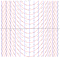 Slope field (black), some solutions (red) and isoclines (blue) of y'=x
 -
 Three integral curves for the slope field corresponding to the differential equation dy / dx = x2 − x − 2


Visualisation of vector field
[edit | edit source]Plot types (Visualization Techniques for Flow Data) : [20]
- Glyphs = Icons or signs for visualizing vector fields
- simplest glyph = Line segment (hedgehog plots)
- arrow plot = quiver plot = Hedgehogs (global arrow plots)
- Characteristic Lines [21]
- streamlines = curve everywhere tangential to the instantaneous vector (velocity) field (time independent vector field). For time independent vector field streaklines = Path lines = streak lines [22]
- texture (line integral convolution = LIC)[23]
- Topological skeleton [24]
- fixed point extraction ( Jacobian)
-
 LIC
LIC -
 Streamlines and streamtube
 -
 Image-based flow visualization
 -
Integral Curves
-
 integral curves
.png)


"path lines, streak lines, and stream lines are identical for stationary flows" Leif Kobbelt[25]
quiver plot
[edit | edit source]Definition
- "A quiver plot displays velocity vectors as arrows with components (u,v) at the points (x,y)"[26]
stream plot
[edit | edit source]- A stream plot uses stream lines
- wolfram: ComplexStreamPlot
Example fields
[edit | edit source]flowmaps
[edit | edit source]- FlowMap Painter by TECK LEE TAN
- Flowmaps, gradient maps, gas giants by Martin Donald
- godot game engine
fBM
[edit | edit source]fBM stands for Fractional Brownian Motion
SDF
[edit | edit source]SDF = Signed Distance Function[27]
- by dimension ( 1D, 2D, 3D, ...)
- by color
- by distance function ( Euclid distance,
- algorithm [28]
- the efficient fast marching method,
- ray marching [29]
- like Marching Parabolas, a linear-time CPU-amenable algorithm.
- Min Erosion, a simple-to-implement GPU-amenable algorithm
- fast sweeping method
- the more general level-set method.
- the efficient fast marching method,
- visualisation ( gray gradient, LSM,
- simple predefined figures or arbitrary shape
It is not
- Sqlce Database File (.SDF) is a database created and accessed by SQL Server Compact Edition. = sdf tag in SO
- SDFormat (Simulation Description Format), sometimes abbreviated as SDF, is an XML format that describes objects and environments for robot simulators, visualization, and control.
- ScientificDataFormat (SDF) and SDF python package = to read, write and interpolate multi-dimensional data. The Scientific Data Format is an open file format based on HDF5 to store multi-dimensional data such as parameters, simulation results or measurements.
- SuiteCloud Development Framework (SDF)
single channel color
[edit | edit source]- SDF for 2d primitives
- normals to SDF
- gradient
- i quilezles : interior distance ( SDF)
- Glyphs, shapes, fonts, signed distance fields by Martin Donald
- CSC2547 DeepSDF Learning Continuous Signed Distance Functions for Shape Representation
- 2D Signed Distance Field Basics by Ronja
- snelly is a WebGL SDF pathtracer by Jamie Portsmouth
- shadertoy : SDF Raymarch Quadtree by paniq
- WGSL 2D SDF Primitives by munrocket
- Define 3 shapes via there Signed Distance Function
- Signed_distance_function in wikipedia
- dist functions 2d by I Quilez
- i quilez : dist grad functions 2d
- SDF
- 8-points Signed Sequential Euclidean Distance Transform
- Distance Transforms of Sampled Functions
- heman
multichannel
[edit | edit source]- Chlumsky: msdfgen =Multi-channel signed distance field generator
- image-sdf = Command-line tool which takes a 4-channel RGBA image and generates a signed distance field. The bitmask is determined by pixels with alpha over 128 and any RGB channel over 128.
mesh
[edit | edit source]- fogleman sdf Simple SDF mesh generation in Python
- christopher batty SDFGen A simple commandline utility to generate grid-based signed distance field (level set) generator from triangle meshes,
Adaptively Sampled Distance Fields
[edit | edit source]
deep
[edit | edit source]fonts, glyphs
[edit | edit source]circle
[edit | edit source]- Disk - distance 2D by iq -good code
- Shader Tutorial | Intro to Signed Distance Fields by Suboptimal Engineer code is not working in actual shadertoy
- c code
- WGLS
// The MIT License
// Copyright © 2020 Inigo Quilez
// Permission is hereby granted, free of charge, to any person obtaining a copy of this software and associated documentation files (the "Software"), to deal in the Software without restriction, including without limitation the rights to use, copy, modify, merge, publish, distribute, sublicense, and/or sell copies of the Software, and to permit persons to whom the Software is furnished to do so, subject to the following conditions: The above copyright notice and this permission notice shall be included in all copies or substantial portions of the Software. THE SOFTWARE IS PROVIDED "AS IS", WITHOUT WARRANTY OF ANY KIND, EXPRESS OR IMPLIED, INCLUDING BUT NOT LIMITED TO THE WARRANTIES OF MERCHANTABILITY, FITNESS FOR A PARTICULAR PURPOSE AND NONINFRINGEMENT. IN NO EVENT SHALL THE AUTHORS OR COPYRIGHT HOLDERS BE LIABLE FOR ANY CLAIM, DAMAGES OR OTHER LIABILITY, WHETHER IN AN ACTION OF CONTRACT, TORT OR OTHERWISE, ARISING FROM, OUT OF OR IN CONNECTION WITH THE SOFTWARE OR THE USE OR OTHER DEALINGS IN THE SOFTWARE.
// GSLS

// Signed distance to a disk

// List of some other 2D distances: https://www.shadertoy.com/playlist/MXdSRf
//
// and iquilezles.org/articles/distfunctions2d


float sdCircle( in vec2 p, in float r )
{
    return length(p)-r;
}


void mainImage( out vec4 fragColor, in vec2 fragCoord )
{
	vec2 p = (2.0*fragCoord-iResolution.xy)/iResolution.y;
    vec2 m = (2.0*iMouse.xy-iResolution.xy)/iResolution.y;

	float d = sdCircle(p,0.5);

	// coloring
    vec3 col = (d>0.0) ? vec3(0.9,0.6,0.3) : vec3(0.65,0.85,1.0); // exterior / interior
    col *= 1.0 - exp(-6.0*abs(d)); // adding a black outline ( gray gradient) to the circle
	col *= 0.8 + 0.2*cos(150.0*d); //  adding waves
	col = mix( col, vec3(1.0), 1.0-smoothstep(0.0,0.01,abs(d)) ); // note: adding white border to the circle


	fragColor = vec4(col,1.0);
}
hg_sdf
[edit | edit source]hg_sdf: A glsl library for building signed distance functions
- mercury -
- ink4
- NVScene 2015 Session: How to Create Content with Signed Distance Functions (Johann Korndörfer)
- alan zucconi: signed-distance-functions
- jcowles - A WebGL friendly port of Mercury's hg_sdf library
blender
[edit | edit source]- b3dsdf = A toolkit of 2D/3D distance functions, sdf/vector ops and various utility shader nodegroups (159+) for Blender 2.83+.
Potential of Mandelbrot set
[edit | edit source]-
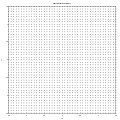 ( Empty) field : points of rectangular mesh
 -
 Scalar field : potential of Mandelbrot set
 -
 Vector field: Array plot of the gradient


Programs
[edit | edit source]- First order, autonomous systems of ODEs
- Runge-Kutta for systems of ODEs
- The geometry and numerics of first order ODEs
- flow-lines by MAKS SURGUY
- symbolab : ordinary-differential-equation-calculator
- PETSc - the Portable, Extensible Toolkit for Scientific Computation, pronounced PET-see (/ˈpɛt-siː/), is for the scalable (parallel) solution of scientific applications modeled by partial differential equations. It has bindings for C, Fortran, and Python (via petsc4py). PETSc also contains TAO, the Toolkit for Advanced Optimization, software library. It supports MPI, and GPUs through CUDA, HIP or OpenCL, as well as hybrid MPI-GPU parallelism; it also supports the NEC-SX Tsubasa Vector Engine.
- Maxima CAS
- CGAL - 2D_Placement_of_Streamlines by Abdelkrim Mebarki
- Python
- OpenProcessing
- G'MIC - display_quiver
- OpenCV
- dsp.stackexchange: how-to-detect-gradients-in-images - Histogram of Oriented Gradients ( HOG )
- arrowed line
- Maxima CAS
- plotdf ( for ODE)
- C++
- par_streamlines ( C, WebGl) by Philip Allan Rideout, github: prideout/par
- JavaScript
- c
- vfplot - program for plotting two-dimensional vector fields by J J Green
- rk4, a C code which implements a fourth-order Runge-Kutta method to solve an ordinary differential equation (ODE). by j burkardt
- gsl
- js
Examples
[edit | edit source]Images
[edit | edit source]- images from commons : Category:Field_lines
- images from commons : Category:Vector_fields
- fractalforums.org : cruising-through-fractal-flow-fields
Shadertoy
[edit | edit source]- tag: vector field
- arrows = quiver plot
- Line Integral Convolution (LIC)
- 3D vector field
Videos
[edit | edit source]- by Chris Thomasson
- Numerical Approximations of Gradients from Deeplearning.ai
- Sticking to the pointy ends: electric field lines in an evolving Julia set capacitor by Nils Berglund
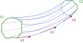
rboyce1000
[edit | edit source]The coloured curves are the separatrices (i.e. real flow lines reaching infinity) of the complex ODE dz/dt = p(z) = z^4 + O(z^2), where the four roots of p(z) are pictured as the black dots: one fixed at the origin, and the remaining three forming the vertices of an equilateral triangle centered at the origin and rotating. Bifurcation occurs at certain critical angles of the rotation, where separatrices instantaneously merge to form homoclinic orbits. Following bifurcation, the so-called 'sectorial pairing' is permuted. There are a total of 5 possible sectorial pairings for the quartic polynomial vector fields (enumerated by the 3rd Catalan number). Three out of the five possibilities can be seen in 2/3 video, while the remaining two can be seen in part 1/3 In 3/3 example, at a bifurcation we have that either: only two of the four roots are centers (the other two remaining attached to separatrices), or NONE of the roots are centers (a phenomenon which does not occur for the quadratic or cubic polynomial vector fields). This video is inspired by the work of A. Douady and P. Sentenac. ( rboyce1000)
Algorithm
- create polynomial with desired properities
- f(z) = z*g(z) with root at origin
- g(z) is a 3-rd root of unity =

f(z) = z(z^3 - 1)
One can check it with Maxima CAS
 z:x+y*%i;
(%o1)                              %i y + x
(%i2) p:z*(z^3-1);
                                               3
(%o2)                    (%i y + x) ((%i y + x)  - 1)
(%i3) display2d:false;

(%o3) false
(%i4) r:realpart(p);

(%o4) x*((-3*x*y^2)+x^3-1)-y*(3*x^2*y-y^3)
(%i5) m:imagpart(p);

(%o5) x*(3*x^2*y-y^3)+y*((-3*x*y^2)+x^3-1)
(%i6) plotdf([r,m],[x,y]);

(%o6) "/tmp/maxout28945.xmaxima"

(%i8) s:solve([p],[x,y]);

(%o8) [[x = %r1,y = (2*%i*%r1+%i+sqrt(3))/2],
       [x = %r2,y = (2*%i*%r2+%i-sqrt(3))/2],[x = %r3,y = %i*%r3],
       [x = %r4,y = %i*%r4-%i]]
to rotate it around origin let's change 1 with : ( multiplier of the fixed point) where t is a proper fraction in turns


Original function from comments:

See also
[edit | edit source]References
[edit | edit source]- ↑ Vector field in wikipedia
- ↑ Euclidian vector in wikipedia
- ↑ matlab : gradient function
- ↑ stackoverflow question: is-there-any-standard-way-to-calculate-the-numerical-gradient
- ↑ nnp_numerical_gradient by Mamy Ratsimbazafy
- ↑ matrixlab-examples : gradient
- ↑ matlab-function-gradient-numerical-gradient by itectec
- ↑ numDeriv : grad
- ↑ numpy : gradient
- ↑ Numerical Methods for Particle Tracing in Vector Fields by Kenneth I. Joy
- ↑ curve sketching by David Guichard and friends
- ↑ liruics : Introduction to Scientific Visualization - Flow Field
- ↑ raster-algorithms-basic-computer-graphics-part-2 by what-when-how
- ↑ bolster.academy : Euler's method interactive
- ↑ interactive Runge Kutta 4 by Greg Petrics
- ↑ grasshopper3d forum: field-lines-how-to-rebuild-and-make-periodic?overrideMobileRedirect=1
- ↑ Classification and visualisation of critical points in 3d vector fields. Master thesis by Furuheim and Aasen
- ↑ Classification and visualisation of critical points in 3d vector fields. Master thesis by Furuheim and Aasen
- ↑ Weisstein, Eric W. "Integral Curve." From MathWorld--A Wolfram Web Resource
- ↑ Flow Visualisation from TUV
- ↑ Data visualisation by Tomáš Fabián
- ↑ A Streakline Representation of Flow in Crowded Scenes from UCF
- ↑ lic by Zhanping Liu
- ↑ Vector Field Topology in Flow Analysis and Visualization by Guoning Chen
- ↑ Vector Field Visualization by Leif Kobbelt
- ↑ matlab ref : quiver plot
- ↑ CedricGuillemet: SDF = Collection of resources (papers, links, discussions, shadertoys,...) related to Signed Distance Field
- ↑ Distance Fields by Philip Rideout in 2018
- ↑ ray-march = Rendering procedural 3D geometry by raymarching through a distance field
- How I built a wind map with WebGL by Vladimir Agafonkin
- math.stackexchange question : what-do-polynomials-look-like-in-the-complex-plane
- mathematica.stackexchange question : visualizing-a-complex-vector-field-near-poles
- fractalforums.com : smooth-external-angle-of-mandelbrot-set
- J.M. Hyman, M. Shashkov, Natural discretizations for the divergence, gradient, and curl on logically rectangular grids, Computers & Mathematics with Applications, Volume 33, Issue 4, 1997, Pages 81-104, ISSN 0898-1221