Fractals/Iterations in the complex plane/equipotetential

Boundary tracing, also known as contour tracing, of a binary digital region can be thought of as a segmentation technique that identifies the boundary pixels of the digital region. Boundary tracing is an important first step in the analysis of that region. Boundary is a topological notion. However, a digital image is no topological space. Therefore, it is impossible to define the notion of a boundary in a digital image mathematically exactly. Most publications about tracing the boundary of a subset S of a digital image I describe algorithms which find a set of pixels belonging to S and having in their direct neighborhood pixels belonging both to S and to its complement I - S. According to this definition the boundary of a subset S is different from the boundary of the complement I – S which is a topological paradox. To define the boundary correctly it is necessary to introduce a topological space corresponding to the given digital image. Such space can be a two-dimensional abstract cell complex. It contains cells of three dimensions: the two-dimensional cells corresponding to pixels of the digital image, the one-dimensional cells or “cracks” representing short lines lying between two adjacent pixels, and the zero-dimensional cells or “points” corresponding to the corners of pixels. The boundary of a subset S is then a sequence of cracks and points while the neighborhoods of these cracks and points intersect both the subset S and its complement I – S. The boundary defined in this way corresponds exactly to the topological definition and corresponds also to our intuitive imagination of a boundary because the boundary of S should contain neither elements of S nor those of its complement. It should contain only elements lying between S and the complement. This are exactly the cracks and points of the complex. This method of tracing boundaries is described in the book of Vladimir A. Kovalevsky and in the web site.

images

• Internal and external LCM
• 
  period 1
• 
  period 1, cubic map
• 
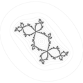
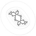
  period 2
• 
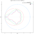
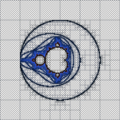
  period 2 with inversed plane
• 
  period 3

• 
• 
• 
• 
• 
• 
• 
• 
• 
  Divide and conquere
• 
• 

Dictionary

• potential
  • scalar potential
  • complex potential
• Contour line, isoline in wikipedia
• equipotential
• tracing
• contour plotting algorithm

Application

• boundary tracing
• shape of the function f = shape of the critical level curves (level curves containing critical points of f)

Algorithms

Algorithms used for boundary tracing:

• Square tracing algorithm
• Moore-neighbor tracing algorithm
• Radial sweep
• Theo Pavlidis’ algorithm
• A generic approach using vector algebra for tracing of a boundary can be found at.
• An extension of boundary tracing for segmentation of traced boundary into open and closed sub-section is described at.
• edge detection of level sets boundaries: Level Set Method (LSM) + edge detection ( for example Sobel filter)
• tracing equilevel curves ( isocurves)
• inverse iteration of closed curve ( circle) around attractor

Input

• function f(x,y)
  • math equation ( for symbolic computations)
  • program subroutine ( for numerical computations)
• plane
  • matrix of floating-point values ( scalar field ) ( for numerical computations)

Moore-neighbor tracing algorithm

The Moore neighborhood is composed of nine cells: a central cell and the eight cells which surround it.

In cellular automata, the Moore neighborhood is defined on a two-dimensional square lattice and is composed of a central cell and the eight cells that surround it.

The neighborhood is named after Edward F. Moore, a pioneer of cellular automata theory.

Importance

It is one of the two most commonly used neighborhood types, the other one being the von Neumann neighborhood, which excludes the corner cells. The well known Conway's Game of Life, for example, uses the Moore neighborhood. It is similar to the notion of 8-connected pixels in computer graphics.

The Moore neighbourhood of a cell is the cell itself and the cells at a Chebyshev distance of 1.

The concept can be extended to higher dimensions, for example forming a 26-cell cubic neighborhood for a cellular automaton in three dimensions, as used by 3D Life. In dimension d, where $0\leq d,d\in \mathbb {Z}$, the size of the neighborhood is 3^d − 1.

In two dimensions, the number of cells in an extended Moore neighbourhood, given its range r is (2r + 1)².

Algorithm

The idea behind the formulation of Moore neighborhood is to find the contour of a given graph. This idea was a great challenge for most analysts of the 18th century, and as a result an algorithm was derived from the Moore graph which was later called the Moore Neighborhood algorithm.

The pseudocode for the Moore-Neighbor tracing algorithm is

Input: A square tessellation, T, containing a connected component P of black cells.
Output: A sequence B (b1, b2, ..., bk) of boundary pixels i.e. the contour.
Define M(a) to be the Moore neighborhood of pixel a.
Let p denote the current boundary pixel.
Let c denote the current pixel under consideration i.e. c is in M(p).
Let b denote the backtrack of c (i.e. neighbor pixel of p that was previously tested)
 
Begin
  Set B to be empty.
  From bottom to top and left to right scan the cells of T until a black pixel, s, of P is found.
  Insert s in B.
  Set the current boundary point p to s i.e. p=s
  Let b = the pixel from which s was entered during the image scan.
  Set c to be the next clockwise pixel (from b) in M(p).
  While c not equal to s do
    If c is black
      insert c in B
      Let b = p
      Let p = c
      (backtrack: move the current pixel c to the pixel from which p was entered)
      Let c = next clockwise pixel (from b) in M(p).
    else
      (advance the current pixel c to the next clockwise pixel in M(p) and update backtrack)
      Let b = c
      Let c = next clockwise pixel (from b) in M(p).
    end If
  end While
End

Termination condition

The original termination condition was to stop after visiting the start pixel for the second time. This limits the set of contours the algorithm will walk completely. An improved stopping condition proposed by Jacob Eliosoff is to stop after entering the start pixel for the second time in the same direction you originally entered it.

tracing by David Rand

Description by David Rand

The plotting algorithm can be summarized thus:

a) Given a matrix of floating point values which are the values of a function z = f(x,y) given at the nodes of a grid of x and y values (the grid values are assumed equally spaced, although the horizontal and vertical spacing may differ), the program determines the minimum and maximum values of z and then computes a number of contour values (in this implementation, 10 values) by linear or logarithmic interpolation between the extrema.

b) The program "walks" about the grid of points looking for any segment (i.e. a line joining two adjacent nodes in the grid) which must be crossed by one of the contours because some contour value lies between the values of z at the nodes.

c) Having found such a segment, it finds the intersection point of the contour and the segment by linear interpolation between the nodes. It also stores the information that the current contour value has been located on the current segment, so that this operation will not be repeated.

d) The program then attempts to locate a neighbouring segment having a similar property - that is, crossed by the same contour. If it finds one, it determines the intersection point as in step c) and then draws a straight line segment joining the previous intersection point with the current one. This step is repeated until no such neighbour can be found, taking care to exclude any segment which has already been dealt with.

e) Steps b), c) and d) are repeated until no segment can be found whose intersection with any contour value has not already been processed.

Square tracing algorithm

The square tracing algorithm is simple, yet effective. Its behavior is completely based on whether one is on a black, or a white cell (assuming white cells are part of the shape). First, scan from the upper left to right and row by row. Upon entering your first white cell, the core of the algorithm starts. It consists mainly of two rules:

• If you are in a white cell, go left.
• If you are in a black cell, go right.

Keep in mind that it matters how you entered the current cell, so that left and right can be defined.

public void GetBoundary(byte[,] image)
{
    for (int j = 0; j < image.GetLength(1); j++)
        for (int i = 0; i < image.GetLength(0); i++)
            if (image[i, j] == 255)               // Found first white pixel
                SquareTrace(new Point(i, j));
}

public void SquareTrace(Point start)
{
    HashSet<Point> boundaryPoints = new HashSet<Point>();  // Use a HashSet to prevent double occurrences
    // We found at least one pixel
    boundaryPoints.Add(start);

    // The first pixel you encounter is a white one by definition, so we go left. 
    // Our initial direction was going from left to right, hence (1, 0)
    Point nextStep = GoLeft(new Point(1, 0));               
    Point next = start + nextStep;
    while (next != start)
    {
        // We found a black cell, so we go right and don't add this cell to our HashSet
        if (image[next.x, next.y] == 0)
        {
            next = next - nextStep;
            nextStep = GoRight(nextStep);
            next = next + nextStep;
        }
        // Alternatively we found a white cell, we do add this to our HashSet
        else
        {
            boundaryPoints.Add(next);
            nextStep = GoLeft(nextStep);
            next = next + nextStep;
        }
    }
}

private Point GoLeft(Point p) => new Point(p.y, -p.x);
private Point GoRight(Point p) => new Point(-p.y, p.x);

Test values

• on the parameter plane
  • c = -0.752174630125934 +0.057670473174377*i. Potential = 2.108396223015232e-16
  • c = -0.750087705298239 +0.014275963195317 *i, ( Mandel can not draw such equipotential line)

Programs

• otis by Tomoki Kawahira
• mandel by Wolf Jung
• ofxContourPlot by Eva Schindling- contour-plotting of mathematical functions f(x,y)
• xd3d
• Fractal zoomer

Code

• C++ code from Mandel by Wolf Jung
• Contour tracing library : A 2D library to trace contours. by STPR.
• Implementation of the paper "Topological Structural Analysis of Digitized Binary Images by Border Following" using C language
• A-C-implementation-of-an-improved-contour-plotting ( c++)
• contour lines
  • in Maxima CAS
• conplot in Fortran
• Paul Bourke: conrec
• c code
• d3 - js library
• Implementation of an Improved Contour Plotting Algorithm August 1981 Thesis by Michael Faiman

Lisp

Lisp code from Maxima CAS

Function ploteq

 ploteq (exp, ...options...)

plots equipotential curves for exp, which should be an expression depending on two variables. The curves are obtained by integrating the differential equation that define the orthogonal trajectories to the solutions of the autonomous system obtained from the gradient of the expression given. The plot can also show the integral curves for that gradient system (option fieldlines).

This program also requires Xmaxima, even if its run from a Maxima session in a console, since the plot will be created by the Tk scripts in Xmaxima. By default, the plot region will be empty until the user clicks in a point (or gives its coordinate with in the set-up menu or via the trajectory_at option).

Most options accepted by plotdf can also be used for ploteq and the plot interface is the same that was described in plotdf.

Example:

  load("plotdf.lisp")$
  V: 900/((x+1)^2+y^2)^(1/2)-900/((x-1)^2+y^2)^(1/2)$
  ploteq(V,[x,-2,2],[y,-2,2],[fieldlines,"blue"])$

Clicking on a point will plot the equipotential curve that passes by that point (in red) and the orthogonal trajectory (in blue).

source code files:

• share/dynamics/dynamics.mac
• share/diffequations/drawdf.mac
• share/dynamics/plotdf.lisp

;; plotdf.mac - Adds a function plotdf() to Maxima, which draws a Direction
;;              Field for an ordinary 1st order differential equation,
;;              or for a system of two autonomous 1st order equations.
;;   
;; Copyright (C) 2004, 2008, 2011 Jaime E. Villate <villate@fe.up.pt>
;;


  
;; plot equipotential curves for a scalar field f(x,y)
(defun $ploteq (fun &rest options)
  
  (let (file cmd mfun (opts " ") (s1 '$x) (s2 '$y))
    (setf mfun `((mtimes) -1 ,fun))
    ;; if the variables are not x and y, their names must be given right
    ;; after the expression for the ode's
    (when
      (and (listp (car options)) (= (length (car options)) 3)
            (or (symbolp (cadar options)) ($subvarp (cadar options)))
            (or (symbolp (caddar options)) ($subvarp (caddar options))))
      (setq s1 (cadar options))
      (setq s2 (caddar options))
      (setq options (cdr options)))
    (defun subxy (expr)
      (if (listp expr)
          (mapcar #'subxy expr)
          (cond ((eq expr s1) '$x) ((eq expr s2) '$y) (t expr))))
    (setf mfun (mapcar #'subxy mfun))
;; the next two lines should take into account parameters given in the options
;;    (if (delete '$y (delete '$x (rest (mfuncall '$listofvars ode))))
;;        (merror "The equation(s) can depend only on 2 variable which must be specified!"))
    (setq cmd (concatenate 'string " -dxdt \""
			   (expr_to_str (mfuncall '$diff mfun '$x))
			   "\" -dydt \""
			   (expr_to_str (mfuncall '$diff mfun '$y)) 
			   "\" "))
    
    ;; parse options and copy them to string opts
    (cond (options
           (dolist (v options) 
             (setq opts (concatenate 'string opts " "
                                  (plotdf-option-to-tcl v s1 s2))))))

    (unless (search "-vectors " opts)
      (setq opts (concatenate 'string opts " -vectors {}")))
    (unless (search "-fieldlines " opts)
      (setq opts (concatenate 'string opts " -fieldlines {}")))
    (unless (search "-curves " opts)
      (setq opts (concatenate 'string opts " -curves {red}")))
    (unless (search "-windowtitle " opts)
      (setq opts (concatenate 'string opts " -windowtitle {Ploteq}")))
    (unless (search "-xaxislabel " opts)
      (setq opts (concatenate 'string opts " -xaxislabel " (ensure-string s1))))
    (unless (search "-yaxislabel " opts)
      (setq opts (concatenate 'string opts " -yaxislabel " (ensure-string s2))))
							      
    (setq file (plot-temp-file (format nil "maxout~d.xmaxima" (getpid))))
    (show-open-plot
     (with-output-to-string
         (st)
       (cond ($show_openplot (format st "plotdf ~a ~a~%" cmd opts))
             (t (format st "{plotdf ~a ~a}" cmd opts))))
     file)
    file))

References

• math.stackexchange question : equipotential-curves-of-a-julia-set
• d3-contour