Local Area Network design/Print version
| This is the print version of Local Area Network design You won't see this message or any elements not part of the book's content when you print or preview this page. |
The current, editable version of this book is available in Wikibooks, the open-content textbooks collection, at
https://en.wikibooks.org/wiki/Local_Area_Network_design
Introduction to Local Area Networks
Origins
[edit | edit source]LAN definition
[edit | edit source]The IEEE 802 working group defined the Local Area Network (LAN) as a communication system through a shared medium, which allows independent devices to communicate together within a limited area, using an high-speed and reliable communication channel.
- Keywords
- shared medium: everyone is attached to the same communication medium;
- independent devices: everyone is peer, that is it has the same privilege in being able to talk (no client-server interaction);
- limited area: everyone is located within the same local area (e.g. corporate, university campus) and is at most some kilometers far one from each other (no public soil crossing);
- high-speed: at that time LAN speeds were measured in Megabit per second (Mbps), while WAN speeds in bit per second;
- reliable: faults are little frequent → checks are less sophisticated to the benefit of performance.
LAN vs. WAN comparison
[edit | edit source]Protocols for Wide Area Networks (WAN) and for Local Area Networks evolved independently until the 80s because purposes were different. In the 90s the IP technology finally allowed to interconnect these two worlds.
- WAN
WANs were born in the 60s to connect remote terminals to the few existing mainframes:
- communication physical medium: point-to-point leased line over long distance;
- ownership of physical medium: the network administrator has to lease cables from government monopoly;
- usage pattern: smooth, that is bandwidth occupancy for long periods of time (e.g. terminal session);
- type of communication: always unicast, multiple communications at the same time;
- quality of physical medium: high fault frequency, low speeds, high presence of electromagnetic disturbances;
- costs: high, also in terms of operating costs (e.g. leasing fee for cables);
- intermediate communication system: required to manage large-scale communications (e.g. telephone switches) → switching devices can fault.
- LAN
LANs appeared at the end of the 70s to share resources (such as printers, disks) among small working groups (e.g. departments):
- communication physical medium: multi-point shared bus architecture over short distance;
- ownership of physical medium: the network administrator owns cables;
- usage pattern: bursty, that is short-term data peaks (e.g. document printing) followed by long pauses;
- type of communication: always broadcast, just one communication at the same time;
- quality of physical medium: greater reliability against failures, high speeds, lower exposure to external disturbances;
- costs: reasonable, concentrated mainly when setting up the network;
- intermediate communication system: not required → lower cost, higher speed, greater reliability, greater flexibility in adding and removing stations.
Communication medium sharing
[edit | edit source]Before the advent of hubs and bridges, the shared communication medium could be implemented in two ways:
- physical broadcast: broadcast-based technologies, such as the bus: the signal sent by a station propagates to all the other stations;
- logical broadcast: point-to-point technologies, such as the token ring: the signal sent by a station arrives at the following station, which duplicates it toward the station after that one, and so on.
- Issues
- privacy: everyone can hear what crosses the shared medium → an addressing system should be made (nowadays: MAC addresses);
- concurrency: just one communication at a time is possible:
- collisions: if two stations transmit simultaneously, the data sent by a station may overlap the data sent by the other one → a mechanism for collision detection and recovery should be made (nowadays: CSMA/CD protocol);
- channel monopolization: in the back-to-back transmission, a station may occupy the channel for a long period of time preventing other stations from talking → a sort of statistical multiplexing, that is simulating multiple communications at the same time by defining a maximum transmission unit called chunk and by alternating chunks from a station with the ones from another one (nowadays: Ethernet frames), should be made.
Data-link sub-layers
[edit | edit source]In LANs the data-link layer is split in two sub-layers:
- MAC: it arbitrates the access to the physical medium, and is specific for each physical-layer technology;
- LLC: it defines the interface toward the network layer, and is common in all physical-layer technologies.
MAC
[edit | edit source]Every network card is identified uniquely by a MAC address. MAC addresses have the following format:
| 24 | 48 |
| OUI | NIC ID |
where the fields are:
- Organization Unique Identifier (OUI) field (3 bytes): code assigned uniquely by IEEE to identify the network card manufacturer:
- first least-significant bit in the first byte:[1]
- Individual (value 0): the address is associated to a single station (unicast);
- Group (value 1): the address refers to multiple stations (multicast/broadcast);
- second least-significant bit in the first byte:[1]
- Universal (value 0): the address is assigned uniquely;
- Local (value 1): the address is customized by the user;
- first least-significant bit in the first byte:[1]
- NIC Identifier (NIC ID) field (3 bytes): code assigned uniquely by the manufacturer to identify the specific network card (also called 'Network Interface Controller' [NIC]).
The Media Access Control (MAC) header has the following format:
| 48 | 96 | 112 | 46 to 1500 bytes | 4 bytes |
| Destination Address | Source Address | Length | payload | FCS |
where the fields are:
- Destination Address field (6 bytes): it specifies the destination MAC address.
- This is put before the source MAC address because in this way the destination can process it earlier and discard the frame if it is not addressed to it;
- Source Address field (6 bytes): it specifies the source MAC address (always unicast);
- Length field (2 bytes): it specifies the payload length;
- Frame Control Sequence (FCS) field (4 bytes): it includes the CRC code for integrity control over the entire frame.
- If the CRC code check fails, the arrived frame was corrupted (e.g. because of a collision) and is discarded; higher-layer mechanisms (e.g. TCP) will be responsible for recovering the error by sending again the frame.
A network card when receiving a frame:
- if the destination MAC address matches with the one of the network card or is of broadcast type ('FF-FF-FF-FF-FF-FF'), it accepts it and sends it to higher layers;
- if the destination MAC address does not match with the one of the network card, it discards it.
A network card set in promiscuous mode accepts all frames → it is useful for network sniffing.
LLC
[edit | edit source]The Logical Link Control (LLC) header has the following format:
| 8 | 16 | 24 or 32 |
| DSAP | SSAP | CTRL |
where the fields are:
- DSAP field (1 byte, of which 2 bits reserved): it identifies the upper-layer protocol used by the destination;
- SSAP field (1 byte, of which 2 bits reserved): it identifies the upper-layer protocol used by the source;
- Control (CTRL) field (1 or 2 bytes): it derives from the HDLC control field, but is unused.
- Issues of DSAP and SSAP fields
- limited set of values: just 64 protocols can be coded;
- codes assigned by ISO: just protocol published by an internationally recognized standard organization are corresponding to codes, while protocols defined by other bodies or pushed by some vendors (e.g. IP) are excluded;
- code redundancy: there is no reason to have two fields to defines protocols, because the source and the destination always talk the same protocol (e.g. both IPv4 or both IPv6).
SNAP
[edit | edit source]The Subnetwork Access Protocol (SNAP) is a particular implementation of LLC for protocols which have not a standard code.
The LLC SNAP header has the following format:
| 8 | 16 | 24 | 48 | 64 |
| DSAP (0xAA) | SSAP (0xAA) | CTRL (3) | OUI | Protocol Type |
where the fields are:
- DSAP, SSAP, CTRL fields: LLC fields are fixed to indicate the presence of the SNAP header;
- Organization Unique Identifier (OUI) field (3 bytes): it identifies the organization which defined the protocol.
- If it is equal to 0, the value in the 'Protocol Type' field is corresponding to the one used in Ethernet DIX;
- Protocol Type field (2 bytes): it identifies the upper-layer protocol (e.g. 0x800 = IP, 0x806 = ARP).
Actually, the LLC SNAP header is not very used due to waste of bytes, to the benefit of the 'Ethertype' field in Ethernet DIX.
References
[edit | edit source]- ↑ a b According to the canonical order (network byte order), which is the native order in IEEE 802.3 (Ethernet) but not in IEEE 802.5 (token ring) (please see section Bit-reversed notation in article MAC address on the English Wikipedia).
Ethernet
Ethernet is nowadays the most used technology in wired LANs with shared bus architecture, because it is a simple and little expensive solution with respect to other LAN technologies such as token ring and token bus.
Ethernet frame format
[edit | edit source]Two versions of Ethernet exist, with different frame formats:
- DIX Ethernet II (1982): version developed by DEC, Intel and Xerox (after this the 'DIX' acronym);
- IEEE 802.3 standard (1983): version standardized by the IEEE 802 working group.
Since there are two versions of Ethernet, a considerable inhomogeneity in upper-layer protocol envelopments exists:
- older protocols (e.g. IP) and protocols farther from IEEE use the DIX Ethernet II enveloping;
- protocols standardized since the beginning by IEEE (e.g. STP) use the IEEE 802.3 enveloping.
DIX Ethernet II
[edit | edit source]The DIX Ethernet II packet[1] has the following format:
| 7 bytes | 1 bytes | 6 bytes | 6 bytes | 2 bytes | 46 to 1500 bytes | 4 bytes | 12 bytes |
| preamble | SFD | destination MAC address | source MAC address | EtherType | payload | FCS | IFG |
| DIX Ethernet II frame (64 to 1518 bytes) | |||||||
where the most significant fields are:
- preamble (7 bytes): bit sequence to recover synchronization between the transmitter clock and the receiver clock.
- Preamble can be shortened whenever the packet crosses a hub → it is not possible to connect more than 4 hubs in a cascade:
 Local Area Network design/Repeaters and bridges#Interconnection at the physical layer;
- Start of Frame Delimiter (SFD) field (1 byte): bit sequence identifying the beginning of the frame;
- EtherType field (2 bytes): it identifies the upper-layer protocol used in the payload (it is a number greater or equal to 1500);
- Inter-Frame Gap (IFG) field (12 bytes): pause, that is no signal, identifying the end of the frame.
IEEE 802.3
[edit | edit source]The IEEE 802.3 packet can have one of the two following formats:
| 7 bytes | 1 byte | 14 bytes | 3 bytes | 0 to 1497 bytes | 0 to 43 bytes | 4 bytes | 12 bytes |
| preamble | SFD | MAC header | LLC header | payload | padding | FCS | IFG |
| IEEE 802.3 frame (64 to 1518 bytes) | |||||||
| 7 bytes | 1 byte | 14 bytes | 8 bytes | 0 to 1492 bytes | 0 to 38 bytes | 4 bytes | 12 bytes |
| preamble | SFD | MAC header | LLC SNAP header | payload | padding | FCS | IFG |
| IEEE 802.3 frame (64 to 1518 bytes) | |||||||
- Remarks
- the DIX Ethernet II and IEEE 802.3 frames have the same minimum and maximum lengths, because IEEE had to specify a frame format compatible with the old version of Ethernet;
- a DIX Ethernet II frame and an IEEE 802.3 frame can be distinguished by looking at the value in the field following the source MAC address:
- if it is lower or equal to 1500 ('Length' field), the frame is IEEE 802.3;
- if it is greater or equal to 1536 ('EtherType' field), the frame is DIX Ethernet II;
- in the IEEE 802.3 frame the 'Length' field would make superfluous the 'Inter-Frame Gap' (IFG) field, but it is present to keep compatibility with the DIX Ethernet II frame;
- in the DIX Ethernet II frame the upper layer has to transmit at least 46 bytes, while in the IEEE 802.3 frame the frame can be stretched to the minimum size with some padding as needed;
- the LLC and LLC SNAP headers in the IEEE 802.3 frame waste a lot more bytes with respect to the 'EtherType' field in the DIX Ethernet II frame although they are aimed to the same functionality of specifying the upper-layer protocol, and this is why the IEEE 802.3 standard has not been widely adopted to the benefit of DIX Ethernet II.
Physical layer
[edit | edit source]10-Mbps Ethernet can work over the following transmission physical media:
- coaxial cable:
- 10Base5: thick cable (max 500 m);
- 10Base2: thin cable (max 185 m);
- twisted copper pair:
- 10BaseT: cable with 4 twisted pairs of which just 2 used (max 100 m):
- Unshielded (UTP): unshielded;
- Shielded (STP): shielded with single global shield;
- Foiled (FTP): shielded with single global shield + a shield per pair;
- 10BaseT: cable with 4 twisted pairs of which just 2 used (max 100 m):
- optical fiber (max 1-2 km)
Coaxial cable
[edit | edit source]At the beginning shared bus was physically made by a coaxial cable:
- vampire taps: every network card is connected to a thick coaxial cable through a vampire clamp, which allowed electrical propagation via physical contact (galvanic continuity) → uncomfortable connection;
- T-connectors: every network card is connected to a thin coaxial cable through a T-connector → connecting and disconnecting a host requires to unplug the whole network.
Twisted copper pair
[edit | edit source]With the introduction of the twisted copper pair, cabling (that is cable laying in buildings) acquired a greater flexibility: every host can be connected to a RJ45 wall socket through the specific RJ45 connector, and all sockets are in turn connected to a cabinet.
In addition, the RJ11 connector used by telephony can be connected to the RJ45 wall socket, too → in cabling RJ45 sockets can be placed in the whole building and then one can decide whenever whether an Ethernet card or a telephone should be connected, by switching between the data connection and the telephone connection in the cabinet.
Optical fiber
[edit | edit source]- Characteristics
- no sensitivity to electromagnetic interferences
- larger distances
- higher costs
- lower flexibility
CSMA/CD
[edit | edit source]A collision occurs when two or more nodes within the same collision domain transmit at the same time and their signals overlap. The Carrier Sense Multiple Access with Collision Detection (CSMA/CD) protocol specify how to recognize a collision (CD) and how to recover a collision (retransmission).
CSMA/CD is a simple and distributed random-access (that is non-deterministic) protocol: it does not contemplates intermediate devices or particular synchronization mechanisms, unlike token ring where the synchronization mechanism is the token itself → the CSMA/CD protocol is efficient in terms of throughput because there is no overhead for synchronization, in terms of delays and channel occupancy.
In full-duplex mode the CSMA/CD protocol does no longer need to be enabled.
Detecting collisions
[edit | edit source]Instead of transmitting the whole frame and just at the end checking for a collision, the node can use Collision Detection (CD): during the transmission sometimes it tries to understand whether a collision occurred ('listen while talking'), and if so it immediately stops the transmission, avoiding to waste the channel for a useless transmission.
In the real world, collision detection is performed in two different ways depending on the type of transmission medium:
- coaxial cable: there is a single channel for both transmission and reception → measuring the average DC on link is enough;
- twisted copper pair, optical fiber: there are two channels, one for transmission and another for reception:
- transmitting stations: they can realize that a collision occurred by detecting activity on the receiving channel during the transmission;
- non-transmitting stations: they can realize that a collision occurred only by detecting a wrong CRC code on the received frame.
- The jamming sequence is a powerful signal which is sent by who has noticed a collision to guarantee that the CRC code is invalid and to maximize probability that all the other nodes understand that a collision occurred.
Reducing the number of collisions
[edit | edit source]Carrier Sense (CS) allows to reduce the number of collisions: the node which wants to transmit listens to the channel before transmitting:
- if it senses the channel is free: the node transmits the frame;
- if it senses the channel is busy:
- 1-persistent CSMA: the node keeps checking whether the channel is free and transmit as soon as it becomes free;
- 0-persistent CSMA: the node tries again after a random time;
- -persistent CSMA: the node with probability waits a random time (0-persistent), with probability immediately checks again (1-persistent).


In a LAN in the worst case the channel occupancy is equal to 30-40% the available bandwidth → Ethernet implements 1-persistent CSMA/CD because it is aimed for averagely unloaded networks with low probability of collisions.
- CSMA limitations
However, with twisted copper pair or optical fiber CSMA is not able to avoid collisions altogether (otherwise CD would not be useful): if propagation times are considered, a far node can sense the channel as free, even if actually it is busy but transmission has not reached the far node yet:

The vulnerability interval is defined as the time interval where starting a transmission by the far node would create a collision (it is equal to the propagation delay on the channel), and this interval is as larger as distance increases → this protocol works well on small networks.
Recovering collisions
[edit | edit source]After a collision occurred, the frame has to be transmitted again. If the stations involved in the collision transmitted again immediately, another collision would occur → back-off algorithm inserts into the wait a randomness element exponential in retransmissions:
- 1st retransmission: the node waits a time chosen randomly between 0 and 1 slot times;
- 2nd retransmission: the node waits a time chosen randomly from 0 to 3 slot times;
- 3rd retransmission: the node waits a time chosen randomly from 0 to 7 slot times;

and so on, according to formula:

where:
- is the number of collisions occurred on the current frame;
- is the slot time, that is the time required to send an Ethernet frame of minimum size (64 bytes), equivalent to 51.2 µs.


At the end of every wait, the node listens again to the channel by CS.
Constraint between frame size and collision diameter
[edit | edit source]Since the channel access is contended, when one manages to get the network access it is better to transmit large packets. A minimum size for frames needs to be established: if the frame is too small and the collided transmission lasts too little time, it may happen that no stations notice the collision:

A constraint between the frame size and the collision diameter exists so that all collisions are recognized: collision detection works only if the round trip time , that is the outward and return time, is lower than the transmission time :


where is the transmission speed and is the propagation speed.


Increasing the transmission speed means increasing the frame minimum size, or for the same minimum size it means decreasing the maximum distance among nodes, but too large frames would increase the transmission error probability and would clog the network.
In Ethernet DIX the theoretical collision diameter can not exceed 5750 meters:[2]

Without hubs the maximum network size is quite limited by maximum distances supported by transmission media (e.g. due to signal attenuation). Thanks to hubs the network size can be extended (although at most to 3 km due to non-idealities in devices): the hub, typically placed as the star center in a star topology, re-generates the signal (repeater) and internally simulates the shared bus allowing to connect multiple stations together through the twisted copper pair: ![]() Local Area Network design/Repeaters and bridges#Interconnection at the physical layer.
Local Area Network design/Repeaters and bridges#Interconnection at the physical layer.
References
[edit | edit source]- ↑ The standard names the Ethernet frame + the 'Preamble', 'SFD' e 'IFG' fields of the physical layer as 'Ethernet packet'.
- ↑ For frame length preamble and SFD, but not IFG, are considered.
Repeaters and bridges
Interconnection at the physical layer
[edit | edit source]
Repeater and hub[1] are network devices for interconnection at the physical layer, which just receive and propagate a sequence of bits. The interconnected physical-layer channels can also have different technologies (e.g. twisted pair to optical fiber), but all the upper layers must be equal (e.g. Ethernet-only, FDDI-only).
Repeater also performs the function of recovering the signal degradation: it synchronizes itself with the square wave signal and regenerates it so as to clean it. The preamble preceding the frame is used for synchronization, that is signal recognition, and so whenever the signal crosses a repeater a part of this preamble is 'eaten' → it is not possible to connect more than 4 repeaters in a cascade.

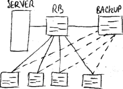
A collision domain is the set of nodes competing to access the same transmissive medium → the simultaneous transmission causes collision. Interconnecting two network segments creates a single collision domain: repeater is not able to recognize collisions which are propagated to all ports → this is a limit to the size of the physical domain.
Interconnection at the data-link layer
[edit | edit source]
Bridge and switch are network devices for interconnection at the data-link layer, which store (store-and-forward mode) and then regenerate the frame. Also the interconnected data-link-layer domains can have different technologies (e.g. Ethernet to FDDI).
- Maximum frame size issue
In practice it is often impossible to interconnect two different data-link-layer technologies, due to issues related to the maximum frame size: for example, in an Ethernet-based network having MTU = 1518 bytes interconnected with a token ring-based network having MTU = 4 KB, what happens if a frame larger than 1518 bytes comes from the token ring network? In addition fragmentation at the data-link layer does not exist.

Bridge decouples broadcast domain from collision domain:
- it 'splits' the collision domain: it implements the CSMA/CD protocol to detect collisions, avoiding propagating them to the other ports;
- it extends the broadcast domain: frames sent in broadcast are propagated to all ports.

Half-duplex and full-duplex modes
[edit | edit source]A point-to-point link at the data-link layer between two nodes (e.g. a host and a bridge) can be performed in two ways:
- half-duplex mode: the two nodes are connected through a single bidirectional wire → each node can not transmit and receive at the same time, because a collision would happen;
- full-duplex mode: the two nodes are connected through two separate unidirectional wires → each node can transmit and receive at the same time, thanks to the splitting of collision domains.
- Full-duplex mode advantages
- higher bandwidth: the throughput between the two nodes doubles;
- absence of collisions:
- the CSMA/CD protocol does no longer need to be enabled;
- the constraint on the minimum Ethernet frame size is no longer needed;
- the limit on the maximum diameter for the collision domain does no longer exist (the only distance limit is the physical one of the channel).
Transparent bridge
[edit | edit source]Routing is performed in a transparent way: the bridge tries to learn the positions of the nodes connected to it filling a forwarding table called filtering database, whose entries have the following format:
where destination port is the port of the bridge, learnt by learning algorithms, which to make frames exit heading towards the associated destination MAC address.
- Learning algorithms
- frame forwarding: learning is based on destination MAC address: when a frame arrives whose destination is not still in the filtering database, the bridge sends the frame in broadcast on all ports but the input port (flooding) and it waits for the reply which the destination is very likely to send back and which the backward learning algorithm will act on;
- backward learning: learning is based on source MAC address: when a frame arrives at a certain port, the bridge checks if there is already the source associated to that port in the filtering database, and if needed it updates it.
Smart forwarding process increases the network aggregate bandwidth: frames are no longer propagated always in broadcast on all ports, but they are forwarded only on the port towards the destination, leaving other links free to transport other flows at the same time.
Mobility
[edit | edit source]Ageing time allows to keep the filtering database updated: it is set to 0 when the entry is created or updated by the backward learning algorithm, and it is increased over time until it exceeds the expiration time and the entry is removed. In this way the filtering database contains information about the only stations which are actually within the network, getting rid of information about old stations.
Data-link-layer networks natively support mobility: if the station is moved, remaining within the same LAN, so as to be reachable through another port, the bridge has to be 'notified' of the movement by sending any broadcast frame (e.g. ARP Request), so that the backward learning algorithm can fix the filtering database. Windows systems tend to be more 'loquacious' than UNIX systems.
Examples of stations which can move are:
- mobile phones;
- virtual machines in datacenters: during the day they can be spread over multiple web servers to distribute the workload, during the night they can be concentrated on the same web server because traffic is lower allowing to save power;
- stations connected to the network via two links, one primary used in normal conditions and one secondary fault-tolerant: when the primary link breaks, the host can restore the connectivity by sending a frame in broadcast through the secondary link.
Switches
[edit | edit source]
'Switch' is the commercial name given to bridges having advanced features to emphasize their higher performance:
- a switch is a multi-port bridge: a switch has a lot more ports, typically all in full-duplex mode, than a bridge;
- the smart forwarding process is no longer a software component but it is implemented into a hardware chip (the spanning tree algorithm keeps being implemented in software because more complex);
- lookup for the port associated to a given MAC address in the filtering database is faster thanks to the use of Content Addressable Memories (CAM), which however have a higher cost and a higher energy consumption;
- switches support cut-through forwarding technology faster than store-and-forward mode: a frame can be forwarded on the target port (unless it is already busy) immediately after receiving the destination MAC address.
Issues
[edit | edit source]Scalability
[edit | edit source]Bridges have scalability issues because they are not able to organize traffic, and therefore they are not suitable for complex networks (such as Wide Area Network):
- no filtering for broadcast traffic → over a wide network with a lot of hosts broadcast frames risk clogging the network;
- the spanning tree algorithm make completely unused some links which would create rings in topology disadvantaging load balancing: Local Area Network design/Spanning Tree Protocol#Scalability.
Security
[edit | edit source]Some attacks to the filtering database are possible:
- MAC flooding attack
The attacking station generates frames with random source MAC addresses → the filtering database gets full of MAC addresses of inexistent stations, while the ones of the existent stations are thrown out → the bridge sends in flooding (almost) all the frames coming from the existent stations because it does not recognize the destination MAC addresses anymore → the network is slowed down and (almost) all the traffic within the network is received by the attacking station.[2]
- Packet storm
The attacking station generates frames with random destination MAC addresses → the bridge sends in flooding all the frames coming from the attacking station because it does not recognize the destination MAC addresses → the network is slowed down.
References
[edit | edit source]- ↑ The difference between repeaters and hubs lies in the number of ports: repeater has two ports, hub has more than two ports.
- ↑ Not all the traffic can be intercepted: when a frame comes from an existent station the bridge saves its source MAC address into its filtering database, so if immediately after a frame arrives heading towards that station, before the entry is cleared, it will not be sent in flooding.
Ethernet evolutions
With the success of Ethernet new issues arose:
- need for higher speed: DIX Ethernet II supported a transmission speed equal to 10 Mbit/s, while FDDI, used in backbone, supported a very higher speed (100 Mbit/s), but it would have been too expensive to wire buildings by optical fiber;
- need to interconnect multiple networks: networks of different technologies (e.g. Ethernet, FDDI, token ring), were difficult to interconnect because they had different MTUs → having the same technology everywhere would have solved this problem.
Fast Ethernet
[edit | edit source]Fast Ethernet, standardized as IEEE 802.3u (1995), raises the transmission speed to 100 Mbit/s and makes the maximum collision diameter 10 times shorter (~200-300 m) accordingly, keeping the same frame format and the same CSMA/CD algorithm.
Physical layer
[edit | edit source]Fast Ethernet physical layer is altogether different than 10-Mbit/s Ethernet physical layer: it partially derives from existing standards in the FDDI world, so much that Fast Ethernet and FDDI are compatible at the physical layer, and definitively abandons the coaxial cable:
- 100BASE-T4: twisted copper pair using 4 pairs;
- 100BASE-TX: twisted copper pair using 2 pairs;
- 100BASE-FX: optical fiber (only in backbone).
Adoption
[edit | edit source]When Fast Ethernet was introduced, its adoption rate was quite low because of:
- distance limit: network size was limited → Fast Ethernet was not appropriate for backbone;
- bottlenecks in backbone: the backbone made in 100-Mbps FDDI technology had the same speed as access networks in Fast Ethernet technology → it was unlikely to be able to drain all the traffic coming from access networks.
Fast Ethernet started to be adopted more widely with:
- the introduction of bridges: they break the collision domain overcoming the distance limit;
- the introduction of Gigabit Ethernet in backbone: it avoids bottlenecks in backbone.
Gigabit Ethernet
[edit | edit source]Gigabit Ethernet, standardized as IEEE 802.3z (1998), rises the transmission speed to 1 Gbit/s and introduces two features, 'Carrier Extension' and 'Frame Bursting', to keep the CSMA/CD protocol working.
Carrier Extension
[edit | edit source]Decuplicating the transmission speed would make the maximum collision diameter 10 more times shorter putting it down to a few tens of meters, too few for cabling → to keep the maximum collision diameter unchanged, the minimum frame size should be increased to 512 bytes[1].
Stretching the minimum frame however would cause an incompatibility issue: in the interconnection of a Fast Ethernet network and a Gigabit Ethernet network by a bridge, minimum-sized frames coming from the Fast Ethernet network could not enter the Gigabit Ethernet network → instead of stretching the frame the slot time, that is the minimum transmission time unit, was stretched: a Carrier Extension made up of padding dummy bits (up to 448 bytes) was appended to all the frames shorter than 512 bytes:
| 7 bytes | 1 byte | 64 to 1518 bytes | 0 to 448 bytes | 12 bytes |
| preamble | SFD | Ethernet II DIX/IEEE 802.3 frame | Carrier Extension | IFG |
| 512 to 1518 bytes | ||||
- Disadvantages
- Carrier Extension occupies the channel with useless bits.
For example with 64-byte-long frames useful throughput is very low: - in newer pure switched networks the full-duplex mode is enabled → CSMA/CD is disabled → Carrier Extension is useless.

Frame Bursting
[edit | edit source]The maximum frame size of 1518 bytes is obsolete by now: in 10-Mbit/s Ethernet the channel occupancy was equal to 1.2 ms, a reasonable time to guarantee the statistical multiplexing, while in Gigabit Ethernet the channel occupancy is equal to 12 µs → collisions are a lot less frequent → to reduce the header overhead in relation to useful data improving efficiency, the maximum frame size could be increased.
Stretching the maximum frame however would cause an incompatibility issue: in the interconnection of a Fast Ethernet network and a Gigabit Ethernet network by a bridge, maximum-sized frames coming from the Gigabit Ethernet network could not enter the Fast Ethernet networks → Frame Bursting consists in concatenating several standard-sized frames one after the other, without realising the channel:
| frame 1[2] + Carrier Extension |
FILL | frame 2[2] | FILL | ... | FILL | last frame[2] | IFG | |
| burst limit (8192 bytes) | ||||||||
- just the first frame is possibly extended by Carrier Extension, to make sure that the collision window is filled; in the next frames Carrier Extension is useless because, if a collision would occur, it would already be detected by the first frame;
- IFG between a frame and another is replaced by a 'Filling Extension' (FILL) to frame bytes and announce that another frame will follow;
- the transmitter station keeps a byte counter: when it arrives to byte number 8192, the frame currently in transmission must be the last one → up to 8191 bytes + 1 frame can be sent with Frame Bursting.
- Advantages
- the number of collision chances is reduced: once the first frame is transmitted without collisions, all the other stations detect that the channel is busy thanks to CSMA;
- the frames following the first one do not require Carrier Extension → useful throughput increases especially in case of small frames, thanks to saving for Carrier Extension.
- Disadvantages
- Frame Bursting does not address the primary goal of reducing the header overhead: it was opted to keep in every frame all headers (including preamble, SFD and IFG) to make the processing hardware simpler;
- typically a station using Frame Bursting has to send a lot of data → big frames do not require Carrier Extension → there is no saving for Carrier Extension;
- in newer pure switched networks the full-duplex mode is enabled → CSMA/CD is disabled → Frame Bursting has no advantages and therefore is useless.
Physical layer
[edit | edit source]Gigabit Ethernet can work over the following transmission physical media:
- twisted copper pair:
- Shielded (STP): the 1000BASE-CX standard uses 2 pairs (25 m);
- Unshielded (UTP): the 1000BASE-T standard uses 4 pairs (100 m);
- optical fiber: the 1000BASE-SX and 1000BASE-LX standards use 2 fibers, and can be:
- Multi-Mode Fiber (MMF): less valuable (275-550 m);
- Single-Mode Fiber (SMF): its maximum length is 5 km.
- GBIC
Gigabit Ethernet introduces for the first time gigabit interface converters (GBIC), which are a common solution for having the capability of updating the physical layer without having to update the rest of the equipment: the Gigabit Ethernet board has not the physical layer integrated on board, but it includes just the logical part (from the data-link layer upward), and the user can plug into the dedicated board slots the desired GBIC implementing the physical layer.
10 Gigabit Ethernet
[edit | edit source]10 Gigabit Ethernet, standardized as IEEE 802.3ae (2002), raises the transmission speed to 10 Gbps and finally abandons the half-duplex mode, removing all the issues deriving from CSMA/CD.
It is not still used in access networks, but it is mainly being used:
- in backbones: it works over optical fiber (26 m to 40 km) because the twisted copper pair is no longer enough because of signal attenuation limitations;
- in datacenters: besides optical fibers, also very short cables are used to connect servers to top-of-the-rack (TOR) switches:[3]
- Twinax: coaxial cables, first used because units for transmission over twisted copper pairs were consuming too much power;
- 10Gbase T: shielded twisted copper pairs, having a very high latency;
- in Metropolitan Area Networks (MAN) and Wide Area Networks (WAN): 10 Gigabit Ethernet can be transported over already existing MAN and WAN infrastructures, although at a transmission speed decreased to 9.6 Gb/s.
40 Gigabit Ethernet and 100 Gigabit Ethernet
[edit | edit source]40 Gigabit Ethernet and 100 Gigabit Ethernet, both standardized as IEEE 802.3ba (2010), raise the transmission speed respectively to 40 Gbit/s and 100 Gbit/s: for the first time the transmission speed evolution is no longer at 10×, but it was decided to define a standard at an intermediate speed due to still high costs for 100 Gigabit Ethernet. In addition, 40 Gigabit Ethernet can be transported over the already existing DWDM infrastructure.
These speeds are used only in backbone because they are not suitable yet not only for hosts, but also for servers, because they are very close to internal speeds in processing units (bus, memory, etc.) → the bottleneck is no longer the network.
References
[edit | edit source]- ↑ In theory the frame should be stretched 10 times more, then to 640 bytes, but the standard decides otherwise.
- ↑ a b c preamble + SFD + Ethernet II DIX/IEEE 802.3 frame
- ↑ Please refer to section FCoE.
Advanced features on Ethernet networks
Autonegotiation
[edit | edit source]Autonegotiation is a plug-and-play oriented feature: when a network card connects to a network, it sends impulses by a particular encoding to try to determine network characteristics:
- mode: half-duplex or full-duplex (over twisted pair);
- transmission speed: starting from the highest speed down to the lowest one (over twisted pair and optical fiber).
- Negotiation sequence
- 1 Gb/s full-duplex
- 1 Gb/s half-duplex
- 100 Mb/s full-duplex
- 100 Mb/s half-duplex
- 10 Mb/s full-duplex
- 10 Mb/s half-duplex
Issues
[edit | edit source]Autonegotiation is possible only if the station connects to another host or to a bridge: hubs in fact work at fixed speed, hence they can not negotiate anything. If during the procedure the other party does not respond, the negotiating station assumes it is connected to a hub → it automatically sets the mode to half-duplex.
If the user manually configures his own network card to work always in full-duplex mode disabling the autonegotiation feature, when he connects to a bridge the latter, not receiving reply from the other party, assumes to be connected to a hub and sets the half-duplex mode → the host considers sending and receiving at the same time over the channel as possible, while the bridge considers that as a collision on the shared channel → the bridge detects a lot of collisions which are false positives, and erroneously discards a lot of frames → every discarded frame is recovered by TCP error-recovery mechanisms, which however are very slow → the network access speed is very low. Very high values in collision counters on a specific bridge port are symptom of this issue.
Increasing the maximum frame size
[edit | edit source]The original Ethernet specification defines:
- maximum frame size: 1518 bytes;
- maximum payload size (MTU): 1500 bytes.
However in several cases it would be useful to have a frame larger than normal:
- additional headers: #Baby Giant frames
- bigger payload: #Jumbo Frames
- less CPU interrupts: #TCP offloading
Baby Giant frames
[edit | edit source]Baby Giant frames are frames having sizes bigger than the maximum size of 1518 bytes defined by the Ethernet original specification, because of inserting new data-link-layer headers in order to transport additional information about the frame:
- frame VLAN tagging (IEEE 802.1Q) adds 4 bytes: Local Area Network design/Virtual LANs#Frame tagging;
- VLAN tag stacking (IEEE 802.1ad) adds 8 bytes: Local Area Network design/Virtual LANs#Tag stacking;
- MPLS adds 4 bytes per stacked label: Computer network technologies and services/MPLS#MPLS header.
In Baby Giant frames the maximum payload size (e.g. IP packet) is unchanged → a router, when receiving a Baby Giant frame, in re-generating the data-link layer can envelop the payload into a normal Ethernet frame → interconnecting LANs having different supported frame maximum sizes is not a problem.
The IEEE 802.3as standard (2006) proposes to extend the maximum frame size to 2000 bytes, keeping the MTU size unchanged.
Jumbo Frames
[edit | edit source]Jumbo Frames are frames having sizes bigger than the maximum size of 1518 bytes defined by the Ethernet original specification:
- Mini Jumbos: frames having MTU size equal to 2500 bytes;
- Jumbos (or 'Giant' or 'Giant Frames'): frames having MTU size up to 9 KB;
because of enveloping bigger payloads in order to:
- transport storage data: typically elementary units of storage data are too big to be transported in a single Ethernet frame:
- the NFS protocol for NASes transports data blocks of about 8 KB;
- the FCoE protocol for SANs and the FCIP protocol for SAN interconnection transport Fibre Channel frames of about 2.5 KB;
- the iSCSI protocol for SANs transports SCSI commands of about 8 KB;
- reduce the header overhead in terms of:
- saving for bytes: it is not very significant, especially considering the high available bandwidth in today's networks;
- processing capability for TCP mechanisms (sequence numbers, timers...): every TCP packet triggers a CPU interrupt.
If a LAN using Jumbo Frames is connected to a LAN not using Jumbo Frames, all Jumbo Frames will be fragmented at the IP layer, but IP fragmentation is not convenient from the performance point of view → Jumbo Frames are used in independent networks within particular scopes.
TCP offloading
[edit | edit source]Network cards with the TCP offloading feature can automatically condense on-the-fly multiple TCP payloads into a single IP packet before turning it to the operating system (sequence numbers and other parameters are internally handled by the network card) → the operating system, instead of having to process multiple small packets by triggering a lot of interrupts, sees a single bigger IP packet and can make the CPU process it at once → this reduces overhead due to TCP mechanisms.
PoE
[edit | edit source]Bridges having the Power over Ethernet (PoE) feature are able to distribute electrical power (up to few tens of Watts) over Ethernet cables (only twisted copper pairs), to connect devices with moderate power needs (VoIP phones, wi-fi access points, surveillance cameras, etc.) avoiding additional cables for electrical power.
Non-PoE stations can be connected to PoE sockets.
Issues
[edit | edit source]- energy consumption: a PoE bridge consumes a lot more electrical power (e.g. 48 ports each one at 25 W consume 1.2 kW) and is more expensive than a traditional bridge;
- service continuity: a failure of the PoE bridge or a power blackout cause telephones, which instead are an important service in case of emergency, to stop working → uninterruptible power supplies (UPS) need to be set but they, instead of providing just traditional telephones with electrical power, have to provide the whole data infrastructure with electrical power.
Spanning Tree Protocol
The loop problem
[edit | edit source]
If the network has a logical ring in topology, some frames may start moving indefinitely in a chain multiplication around the loop:
- broadcast/multicast frames: they are always propagated on all ports, causing a broadcast storm;
- unicast frames sent to a station yet not included in the filtering database or inexistent: they are sent in flooding.
Moreover, bridges in the loop may have their filtering databases inconsistent, that is the entry in the filtering database related to the sender station changes its port every time a frame replication arrives through a different port, making the bridge believe that the frame has come from the station itself moving.
Spanning tree algorithm
[edit | edit source]| This page includes CC BY-SA contents from Wikipedia: Spanning Tree Protocol. |
The spanning tree algorithm allows to remove logical rings from the network physical topology, by disabling links[1] to transform a mesh topology (graph) into a tree called spanning tree, whose root is one of the bridges called root bridge.
Each link is characterized by a cost based on the link speed: given a root bridge, multiple spanning trees can be built connecting all bridges one with each other, but the spanning tree algorithm chooses the spanning tree made up of the lowest cost edges.
- Parameters
- Bridge Identifier: it identifies the bridge uniquely and includes:
- bridge priority: it can be set freely (default value = 32768);
- bridge MAC address: it is chosen between the MAC address of his ports by a vendor-specific algorithm and can not be changed;
- Port Identifier: it identifies the bridge port and includes:
- port priority: it can be set freely (default value = 128);
- port number: in theory a bridge can not have more than 256 ports → in practice also the port priority field can be used if needed;
- Root Path Cost: it is equal to the sum of the costs of all links, selected by the spanning tree algorithm, traversed to reach the root bridge (the cost for traversing a bridge is null).
Criteria
[edit | edit source]The spanning tree can be determined by the following criteria.
Root bridge
[edit | edit source]A root bridge is the root for the spanning tree: all the frames going from one of its sub-trees to another one must cross the root bridge.[2]
The bridge with the smallest Bridge Identifier is selected as the root bridge: the root of the spanning tree will be therefore the bridge with the lowest priority, or if there is a tie the one with the lowest MAC address.
Root port
[edit | edit source]- Criteria for selecting a root port for the bridge the arrow points to.
-
 Least-cost path.
 -
 Smallest remote Bridge ID.
 -
 Smallest remote Port ID.
 -
 Smallest local Port ID.


A root port is the port in charge of connecting to the root bridge: it sends frames toward the root bridge and receives frames from the root bridge.
- The cost of each possible path is determined from the bridge to the root. From these, the one with the smallest cost (a least-cost path) is picked. The port connecting to that path is then the root port for the bridge.
- When multiple paths from a bridge are least-cost paths toward the root, the bridge uses the neighbor bridge with the smallest Bridge Identifier to forward frames to the root. The root port is thus the one connecting to the bridge with the lowest Bridge Identifier.
- When two bridges are connected by multiple cables, multiple ports on a single bridge are candidates for root port. In this case, the path which passes through the port on the neighbor bridge that has the smallest Port Identifier is used.
- In a particular configuration with a hub where the remote Port Identifiers are equal, the path which passes through the port on the bridge itself that has the smallest Port Identifier is used.
Designated port
[edit | edit source]- Criteria for selecting a designated port for the link the arrow points to.
-
 Least-cost path.
 -
 Smallest local Bridge ID.
 -
 Smallest local Port ID.


A designated port is the port in charge of serving the link: it sends frames to the leaves and receives frames from the leaves.
- The cost of each possible path is determined from each bridge connected to the link to the root. From these, the one with the smallest cost (a least-cost path) is picked. The port connected to the link of the bridge which leads to that path is then the designated port for the link.
- When multiple bridges on a link lead to a least-cost path to the root, the link uses the bridge with the smallest Bridge Identifier to forward frames to the root. The port connecting that bridge to the link is the designated port for the link.
- When a bridge is connected to a link with multiple cables, multiple ports on a single bridge are candidates for designated port. In this case, the path which passes through the port on the bridge itself that has the smallest Port Identifier is used.
Blocked port
[edit | edit source]A blocked port never sends frames on its link and discards all the received frames (except for BPDU configuration messages).
Any active port that is not a root port or a designated port is a blocked port.

BPDU messages
[edit | edit source]The above criteria describe one way of determining what spanning tree will be computed by the algorithm, but the rules as written require knowledge of the entire network. The bridges have to determine the root bridge and compute the port roles (root, designated, or blocked) with only the information that they have.
Since bridges can exchange information about Bridge Identifiers and Root Path Costs, Spanning Tree Protocol (STP), standardized as IEEE 802.1D (1990), defines messages called BPDUs.
BPDU format
[edit | edit source]BPDUs have the following format:
| 1 | 7 | 8 | 16 | 24 | 32 |
| Protocol ID (0) | Version (0) | BPDU Type (0) | |||
| TC | 000000 | TCA | Root Priority | ||
| Root MAC Address | |||||
| Root Path Cost | |||||
| Bridge Priority | |||||
| Bridge MAC Address | |||||
| Port Priority | Port Number | Message Age | |||
| Max Age | Hello Time | ||||
| Forward Delay | |||||
| 16 | 24 | 32 |
| Protocol ID (0) | Version (0) | BPDU Type (0x80) |
where the fields are:
- Protocol Identifier field (2 bytes): it specifies the IEEE 802.1D protocol (value 0);
- Version field (1 byte): it distinguishes Spanning Tree Protocol (value 0) from Rapid Spanning Tree Protocol (value 2);
- BPDU Type field (1 byte): it specifies the type of BPDU:
- Configuration BPDU (CBPDU) (value 0): used for spanning tree computation, that is to determine the root bridge and the port states: #Ingress of a new bridge;
- Topology Change Notification BPDU (TCN BPDU) (value 0x80): used to announce changes in the network topology in order to update entries in filtering databases: #Announcing topology changes;
- Configuration BPDU (CBPDU) (value 0): used for spanning tree computation, that is to determine the root bridge and the port states:
- Topology Change (TC) flag (1 bit): set by the root bridge to inform all bridges that a change occurred in the network;
- Topology Change Acknowledgement (TCA) flag (1 bit): set by the root bridge to inform the bridge which detected the change that its Topology Change Notification BPDU has been received;
- Root Identifier field (8 bytes): it specifies the Bridge Identifier of the root bridge in the network:
- Root Priority field (2 bytes): it includes the priority of the root bridge;
- Root MAC Address field (6 bytes): it includes the MAC address of the root bridge;
- Bridge Identifier field (8 bytes): it specifies the Bridge Identifier of the bridge which is propagating the Configuration BPDU:
- Bridge Priority field (2 bytes): it includes the priority of the bridge;
- Bridge MAC Address field (6 bytes): it includes the MAC address of the bridge;
- Root Path Cost field (4 bytes): it includes the path cost to reach the root bridge, as seen by the bridge which is propagating the Configuration BPDU;
- Port Identifier field (2 bytes): it specifies the Port Identifier of the port which the bridge is propagating the Configuration BPDU on:
- Port Priority field (1 byte): it includes the port priority;
- Port Number field (1 byte): it includes the port number;
- Message Age field (2 bytes): value, initialized to 0, which whenever the Configuration BPDU crosses a bridge is increased by the transit time throughout the bridge;[3]
- Max Age field (2 bytes, default value = 20 s): if the Message Age reaches the Max Age value, the received Configuration BPDU is no longer valid;[3]
- Hello Time field (2 bytes, default value = 2 s): it specifies how often the root bridge generates the Configuration BPDU;[3]
- Forward Delay field (2 bytes, default value = 15 s): it specifies the waiting time before forcing a port transition to another state.[3]
BPDU generation and propagation
[edit | edit source]Only the root bridge can generate Configuration BPDUs: all the other bridges simply propagate received Configuration BPDUs on all their designated ports. Root ports are the ones that receive the best Configuration BPDUs, that is with the lowest Message Age value = lowest Root Path Cost. Blocked ports never send Configuration BPDUs but keep listening to incoming Configuration BPDUs.
Instead Topology Change Notification BPDUs can be generated by any non-root bridge, and they are always propagated on root ports.
When a bridge generates/propagates a BPDU frame, it uses the unique MAC address of the port itself as a source address, and the STP multicast address 01:80:C2:00:00:00 as a destination address:
| 6 bytes | 6 bytes | 2 bytes | 1 byte | 1 byte | 1 byte | 4 bytes | |
| 01:80:C2:00:00:00 (multicast) | source bridge address (unicast) | ... | 0x42 | 0x42 | 0x03 | BPDU | ... |
| destination MAC address | source MAC address | length | DSAP | SSAP | CTRL | payload | FCS |
Dynamic behavior
[edit | edit source]Port states
[edit | edit source]- Disabled
- A port switched off because no links are connected to the port.
- Blocking
- A port that would cause a loop if it were active. No frames are sent or received over a port in blocking state (Configuration BPDUs are still received in blocking state), but it may go into forwarding state if the other links in use fail and the spanning tree algorithm determines the port may transition to the forwarding state.
- Listening
- The bridge processes Configuration BPDUs and awaits possible new information that would cause the port to return to the blocking state. It does not populate the filtering database and it does not forward frames.
- Learning
- While the port does not yet forward frames, the bridge learns source addresses from frames received and adds them to the filtering database. It populates the filtering database, but does not forward frames.
- Forwarding
- A port receiving and sending data. STP still keeps monitoring incoming Configuration BPDUs, so the port may return to the blocking state to prevent a loop.
| port state | port role | receive frames? | receive and process CBPDUs? | generate or propagate CBPDUs? | update filtering database? | forward frames? | generate or propagate TCN BPDUs? |
|---|---|---|---|---|---|---|---|
| disabled | blocked | no | no | no | no | no | no |
| blocking | yes | yes | no | no | no | no | |
| listening | (on transitioning) | yes | yes | yes | no | no | no |
| learning | designated | yes | yes | yes | yes | no | no |
| root | yes | yes | no | yes | no | sì | |
| forwarding | designated | yes | yes | yes | yes | yes | no |
| root | yes | yes | no | yes | yes | yes |
Ingress of a new bridge
[edit | edit source]When a new bridge is connected to a data-link network, assuming it has a Bridge Identifier highest than the one of the current root bridge in the network:
- at first the bridge, without knowing anything about the rest of the network (yet), assumes to be the root bridge: it set all its ports as designated (listening state) and starts generating Configuration BPDUs on them, saying it is the root bridge;
- the other bridges receive Configuration BPDUs generated by the new bridge and compare the Bridge Identifier of the new bridge with the one of the current root bridge in the network, then they discard them;
- periodically the root bridge in the network generates Configuration BPDUs, which the other bridges receive from their root ports and propagate through their designated ports;
- when the new bridge receives a Configuration BPDU from the root bridge in the network, it learns it is not the root bridge because another bridge having a Bridge Identifier lower than its one exists, then it stops generating Configuration BPDUs and sets the port from which it received the Configuration BPDU from the root bridge as a root port;
- also the new bridge starts propagating Configuration BPDUs, this time related to the root bridge in the network, on all its other (designated) ports, while it keeps receiving Configuration BPDUs propagated by the other bridges;
- when a new bridge receives on a designed port a Configuration BPDU 'best', based on criteria for designated port selection, with respect to the Configuration BPDU it is propagating on that port, the latter stops propagating Configuration BPDUs and turns to blocked (blocking state);
- after a time Forward Delay long, ports still designated and the root port switch from the listening state to the learning one: the bridge starts populating its filtering database, to avoid the bridge immediately starts sending the frames in flooding overloading the network;
- after a time Forward Delay long, designated ports and the root port switch from the learning state to the forwarding one: the bridge can propagate also normal frames on those ports.
Changes in the network topology
[edit | edit source]Recomputing spanning tree
[edit | edit source]When a topology change occurs, STP is able to detect the topology change, thanks to the periodic generation of Configuration BPDUs by the root bridge, and to keep guaranteeing there are no rings in topology, by recomputing if needed the spanning tree, namely the root bridge and the port states.
Link fault
[edit | edit source]When a link (belonging to the current spanning tree) faults:
- Configuration BPDUs which the root bridge is generating can not reach the other network portion anymore: in particular, the designed port for the faulted link does not send Configuration BPDUs anymore;
- the last Configuration BPDU listened to by the blocked port beyond the link 'ages' within the bridge itself, that is its Message Age is increased over time;
- when the Message Age reaches the Max Age value, the last Configuration BPDU listened to expires and the bridge starts over again electing itself as the root bridge: it resets all its ports as designated, and starts generating Configuration BPDUs saying it is the root bridge;
- STP continues analogously to the case previously discussed related to the ingress of a new bridge:
- if a link not belonging to the spanning tree connecting the two network portions exists, the blocked port connected to that link at last will become root port in forwarding state, and the link will join the spanning tree;
- otherwise, if the two network portions can not be connected one with each other anymore, in every network portion a root bridge will be elected.
Insertion of a new link
[edit | edit source]When a new link is inserted, the ports which the new link is connected to become designated in listening state, and start propagating Configuration BPDUs generated by the root bridge in the network → new Configuration BPDUs arrive through the new link:
- if the link has a cost low enough, the bridge connected to the link starts receiving from a non-root port Configuration BPDUs having a Root Path Cost lower than the one from the Configuration BPDUs received from the root port → the root port is updated so that the root bridge can be reached through the best path (based on criteria for root port selection), as well as designated and blocked ports are possibly updated accordingly;
- if the link has a too high cost, Configuration BPDUs crossing it have a too high Root Path Cost → one of the two ports connected to the new link becomes blocked and the other one keeps being designated (based on criteria for designated port selection).
Announcing topology changes
[edit | edit source]When after a topology change STP alters the spanning tree by changing the port states, it does not change entries in filtering databases of bridges to reflect the changes → entries may be out of date: for example, the frames towards a certain destination may keep being sent on a port turned to blocked, until the entry related to that destination expires because its ageing time goes to 0 (in the worst case: 5 minutes!).
STP contemplates a mechanism to speed up the convergence of the network with respect to the filtering database when a topology change is detected:
- the bridge which detected the topology change generates a Topology Change Notification BPDU through its root port towards the root bridge to announce the topology change;[4]
- crossed bridges immediately forward the Topology Change Notification BPDU through their root ports;
- the root bridge generates back a Configuration BPDU with Topology Change and Topology Change Acknowledgement flags set to 1, which after being forwarded back by crossed bridges will be received by the bridge which detected the topology change;[5]
- the root bridge generates on all its designated ports a Configuration BPDU with the Topology Change flag set;
- every bridge, when receiving the Configuration BPDU:
- drops all the entries in its filtering database having ageing times lower than the Forward Delay;
- in turn propagates the Configuration BPDU on all its designated ports (keeping the Topology Change flag set);
- the network temporarily works in a sub-optimal condition because more frames are sent in flooding, until bridges populate again their filtering databases with new paths by learning algorithms.
Issues
[edit | edit source]Performance
[edit | edit source]The STP philosophy is 'deny always, allow only when sure': when a topology change occurs, frames are not forwarded until it is sure that the transient has dead out, that is there are no loops and the network is in a coherent status, also introducing long waiting times at the expense of convergence speed and capability of reaching some stations.
Assuming to follow the timers recommended by the standard, namely:
- the timing values recommended by the standard are adopted: Max Age = 20 s, Hello Time = 2 s, Forward Delay = 15 s;
- the transit time through every bridge by a BPDU does not exceed the TransitDelay = HelloTime ÷ 2 = 1 s;
more than 7 bridges in a cascade between two end-systems can not be connected so that a Configuration BPDU can cross the entire network twice within the Forward Delay: if an eighth bridge was put in a cascade, in fact, in the worst case the ports at the new bridge, self-elected as the root bridge, would turn from the listening state to the forwarding one[6] before the Configuration BPDU coming from the root bridge at the other end of the network can arrive in time at the new bridge:[7]

With the introduction of the learning state, after a link fault the network takes approximately 50 seconds to converge to a coherent state:
- 20 s (Max Age): required for the last Configuration BPDU listened to to expire and for the fault to be detected;
- 15 s (Forward Delay): required for the port transition from the listening state to the learning one;
- 15 s (Forward Delay): required for the port transition from the learning state to the forwarding one.
In addition, achieving a coherent state within the network does not result necessarily in ending the disservice experienced by the user: in fact the fault may reflect also at the application layer, very sensitive to connectivity losses beyond a certain threshold:
- database management systems may start long fault-recovery procedures;
- multimedia networking applications generating inelastic traffic (such as VoIP applications) suffer much from delay variations.
It would be possible to try customizing the values related to timing parameters to increase the convergence speed and extend the maximum bridge diameter, but this operation is not recommended:
- without paying attention one risks reducing network reactivity to topology changes and impairing network functionality;
- at first sight it appears enough to work just on the root bridge because those values are all propagated by the root bridge to the whole network, but indeed if the root bridge changes the new root bridge must advertise the same values → those parameters must actually be updated on all bridges.
Often STP is disabled on edge ports, that is the ports connected directly to the end hosts, to relieve disservices experienced by the user:
- due to port transition delays, a PC connecting to the network would initially be isolated for a time two Forward Delays long;
- connecting a PC represents a topology change → the cleanup of old entries triggered by the announcement of the topology change would considerably increase the number of frames sent in flooding in the network.
However exclusively hosts must be connected to edge ports, otherwise loops in the network could be created → some vendors do not allow this: for example, Cisco's proprietary mechanism PortFast achieves the same objective without disabling STP on edge ports, being able to make them turn immediately to the forwarding state and to detect possible loops on them (that is two edge ports connected one to each other through a direct wire).
Scalability
[edit | edit source]Given a root bridge, multiple spanning trees can be built connecting all bridges one with each other, but the spanning tree algorithm chooses the spanning tree made up of the lowest cost edges. In this way, paths are optimized only with respect to the root of the tree:
- disabled links are altogether unused, but someone still has to pay for keeping them active as secondary links for fault tolerance;
- load balancing is not possible to distribute traffic over multiple parallel links → links belonging to the selected spanning tree have to sustain also the load for the traffic which, if there was not STP, would take a shorter path by crossing disabled links:

An IP network instead is able to organize traffic better: the spanning tree is not unique in the entire network, but every source can compute its own tree and send traffic to the shortest path guaranteeing a higher link load balancing.
Virtual LANs (VLAN) solve this problem by setting up multiple spanning trees.
Unidirectional links
[edit | edit source]STP assumes every link is bidirectional: if a link faults, frames can not be sent in either of two directions. Indeed fiber optical cables are unidirectional → to connect two nodes two optical fiber cables are needed, one for communication in one direction and another for communication in the opposite direction, and a fault on one of the two cables stops only traffic in one direction.
If one of the two unidirectional links faults, a loop may arise on the other link despite STP: Configuration BPDUs are propagated unidirectionally from the root to the leaves → if the direct propagation path breaks, the bridge at the other endpoint stops receiving from that link Configuration BPDUs from the root bridge, then moves the root port to another link and, assuming there is no one on that link, sets the port as designated creating a loop:

Unidirectional Link Detection (UDLD) is a proprietary protocol of Cisco's able to detect whether there are faults on a unidirectional link thanks to a sort of 'ping', and to disable the port ('error disabled' state) instead of electing it as designated.
Positioning the root bridge
[edit | edit source]-
 Optimal configuration.
 -
 Configuration to be avoided.


The location of the root bridge has heavy impact on the network:
- traffic from one side to another one of the network has to cross the root bridge → performance, in terms of aggregate throughput and bandwidth of ports, of the bridge selected as the root bridge should be enough to sustain a high amount of traffic;
- a star topology, where the root bridge is the star center, is to be preferred → every link connect only one bridge to the root bridge:
- more equable link load balancing: the link should not sustain traffic coming from other bridges;
- higher fault tolerance: a fault of the link affects only connectivity for one bridge;
- servers and datacenters should be placed near the root bridge in order to reduce the latency of data communication;
→ the priority needs to be customized to a very low value for the bridge which has to be the root bridge, so as not to risk that another bridge is elected as the root bridge.
The location of the backup bridge, meant to come into play in case of fault of a primary link or of the primary root bridge:
- fault of a primary link: the optimal configuration is a redundant star topology made up of secondary links, where every bridge is connected to the backup bridge by a secondary link;
- fault of the primary root bridge: the priority of the backup root bridge needs to be customized to a value slightly higher than the priority of the primary root bridge too, so as to force that bridge to be elected as the root bridge in case of fault.
Security
[edit | edit source]STP has not built-in security mechanisms against attacks from outside.
- Electing the user's bridge as the root bridge
A user may connect to the network a bridge with a very low priority forcing it to become the new root bridge and changing the spanning tree of the network. Cisco's proprietary feature BPDU Guard allows edge ports to propagate only Configuration BPDUs coming from inside the network, rejecting the ones received from outside (the port goes into 'error disabled' state).
- Rate limit on broadcast storm
Almost all professional bridges have some form of broadcast storm control able to limit the amount of broadcast traffic on ports by dropping excess traffic beyond a certain threshold, but these traffic meters can not distinguish between frames in a broadcast storm and broadcast frames sent by stations → they risk filtering legitimate broadcast traffic, and a broadcast storm is more difficult to be detected.
- Connecting bridges without STP
A single bridge without STP or with STP disabled can start pumping broadcast traffic into the network so that a loop outside the control of STP is created: connecting a bridge port directly to another one of the same bridge, or connecting the user's bridge to two internal bridge of the network through two redundant links, are examples.
- Multiple STP domains
Sometimes two different STP domains, each one with its own spanning tree, should be connected to the same shared channel (e.g. two providers with different STP domains in the same datacenter). Cisco's proprietary feature BPDU Filter disables sending and receiving Configuration BPDUs on ports at domain peripheries, to keep the spanning trees separated.
References
[edit | edit source]- ↑ Really the spanning tree algorithm blocks ports, not links: {{subst:vedi|#Port states}}
- ↑ Please pay attention to the fact that the traffic moving within the same sub-tree does not cross the root bridge.
- ↑ a b c d Time fields are expressed in units of 256th seconds (about 4 ms).
- ↑ The bridge keeps generating the Topology Change Notification BPDU every Hello Time, until it receives the acknowledge.
- ↑ The root bridge keeps generating back the acknowledgement Configuration BPDU for Max Age + Forward Delay.
- ↑ When this constraint was established, the learning state had not been introduced yet and the ports turned directly from the listening state to the forwarding one.
- ↑ Exactly the minimum value for the Forward Delay would be equal to 14 s, but a tolerance 1 s long was contemplated.
Rapid Spanning Tree Protocol
Rapid Spanning Tree Protocol (RSTP), standardized as IEEE 802.1w (2001), is characterized by a greater convergence speed with respect to STP in terms of:
Port roles and states
[edit | edit source]RSTP defines new port roles and states:
- discarding state: the port does not forward frames and it discards the received ones (except for Configuration BPDUs), unifying disabled, blocking and listening states;
- alternate role: the port, in discarding state, is connected to the same link as a designated port of another bridge, representing a fast replacement for the root port;
- backup role: the port, in discarding state, is connected to the same link as a designed port of the same bridge, representing a fast replacement for the designated port;
- edge role: just hosts can be connected to the port, being aimed to reduce, with respect to the classical STP, disservices experienced by users in connecting their hosts to the network.
| port state | port role | receive frames? | receive and process CBPDUs? | generate and propagate CBPDUs? | update filtering database? | forward frames? |
|---|---|---|---|---|---|---|
| discarding | alternate | yes | yes | no | no | no |
| backup | yes | yes | no | no | no | |
| designated[1] | yes | yes | yes | no | no | |
| learning | designated | yes | yes | yes | yes | no |
| root | yes | yes | no | yes | no | |
| forwarding | designated | yes | yes | yes | yes | yes |
| root | yes | yes | no | yes | yes | |
| edge | yes | yes | no | yes | yes |
Configuration BPDU format
[edit | edit source]Configuration BPDU has the following format:
| 1 | 2 | 4 | 6 | 7 | 8 | 12 | 16 | 24 | 32 |
| Protocol ID (0) | Version (2) | BPDU Type (2) | |||||||
| TC | P | R | S | A | TCA | Root Priority | STP Instance | ||
| Root MAC Address | |||||||||
| Root Path Cost | |||||||||
| Bridge Priority | STP Instance | ||||||||
| Bridge MAC Address | |||||||||
| Port Priority | Port Number | Message Age | |||||||
| Max Age | Hello Time | ||||||||
| Forward Delay | |||||||||
where there are some changes with respect to BPDUs in the classical STP:
- Version field (1 byte): it identifies RSTP as version number 2 (in STP it was 0);
- BPDU Type field (1 byte): it identifies the Configuration BPDU always as type 2 (in STP it was 0), since Topology Change Notification BPDUs do no longer exist;[2]
- 6 new flags: they handle the proposal/agreement mechanism:
- Proposal (P) and Agreement (A) flags (1 bit each one): they specify whether the port role is being proposed by a bridge (P = 1) or has been accepted by the other bridge (A = 1);
- 2 flags in Role field (R) (2 bits): they encode the proposed or accepted port role (00 = unknown, 01 = alternate/backup, 10 = root, 11 = designated);
- 2 flags in State field (S) (2 bits): they specify whether the port which the role is being proposed or has been accepted for is in learning (10) or forwarding (01) state;
- Root Identifier and Bridge Identifier fields (8 bytes each one): RSTP includes technical specifications from IEEE 802.1t (2001) which change the format of Bridge Identifier:
- Bridge Priority field (4 bits, default value = 8);
- STP Instance field (12 bits, default value = 0): used in Virtual LANs to enable multiple protocol instances within the same physical network: Local Area Network design/Virtual LANs#PVST;
- Bridge MAC Address field (6 bytes): unchanged from IEEE 802.1D-1998;
- Root Path Cost field (4 bytes): RSTP includes technical specifications from IEEE 802.1t (2001) which change the recommended values for Port Path Cost including new port speeds (up to 10 Tb/s);
- Max Age and Forward Delay fields (2 bytes each one): they are altogether unused in RSTP, but they have been kept for compatibility reasons.
Changes in the network topology
[edit | edit source]Recomputing spanning tree
[edit | edit source]RSTP is characterized by a greater topology convergence speed with respect to the classical STP: in fact it switches from 50 seconds to less than 1 second (order of about 10 ms) if, as was the norm by then when RSTP was standardized, there are just full-duplex point-to-point links (therefore without hubs).
Detection of a link fault
[edit | edit source]When a link fault occurs, its detection by RSTP is faster than the classical STP thanks to a more efficient BPDU handling.
Non-root bridges do not just propagate BPDUs generated by the root bridge: each bridge generates every Hello Time (default: 2 s) a BPDU, with the current root bridge as Root Identifier, even if it has not received the BPDU from the root bridge. If BPDUs have not been received for 3 Hello Time periods, the current BPDU is declared obsolete and a fault is assumed to be occurred on the link which the root port is connected to.
This faster aging of information is useless on modern networks:
- in older networks with hubs, a bridge can not detect at the physical layer a fault between the hub and another bridge → the only way to detect it is realizing that the 'keep-alive' BPDU messages stopped being received;
- in newer networks which are pure switched, a bridge can immediately detect a link fault at the physical layer without waiting 3 Hello Times periods.
Once a bridge detected a link fault, it starts generating its own BPDUs → every neighbor bridge, as soon as it receives on its root port a BPDU from the bridge which is claiming to be the root bridge, instead of discarding it because it is worse than the current one, accepts the new BPDU forgetting the one previously stored, because it means that something bad happened on its path toward the root bridge. At this point:
- if its Bridge Identifier is worse than the one in the BPDU, the bridge starts generating BPDUs on its designated ports with the new Root Identifier;
- if its Bridge Identifier is better than the one in the BPDU, the bridge starts generating its own BPDUs claiming to be the root bridge.
Recovery from a link fault
[edit | edit source]Once a fault is detected, some ports can directly turn to the forwarding state without transitioning across the learning state.
- Alternate ports
In case the root port faults, the alternate port provides an alternative path between the bridge and the root bridge:
- The alternate port represents a fast replacement for the root port.
-

-

- Backup ports
In case a designed port faults, the backup port provides an alternative path between the bridge and the link:
- The backup port represents a fast replacement for the designated port.
-

-


Insertion of a new link
[edit | edit source]The proposal/agreement sequence is an algorithm for fast synchronization on the port role between two bridges.
When a new link is inserted between two bridges:
- each of the two bridges puts into discarding state its port connected to the new link, as well as all its possible other root and designated ports connected on other links, to prevent creation of possible loops during the transient;
- each of the two bridges proposes its port as designated for the link by sending a BPDU to the new link with the Proposal flag set;
- the worse bridge accepts the proposal from the other bridge by sending back a BPDU with the Agreement flag set, and puts its port into the proper role (root, alternate, or backup) according to spanning tree algorithm criteria;
- the best bridge receives the acceptance BPDU and puts its port as designated for the link;
- each of the two bridges repeats the sequence for the other ports which at the beginning it put into discarding state.
Cooperation between the two bridges through BPDU sending is faster with respect to the timer-based mechanism in the classical STP, and more efficient since it does not stop the whole network for a while but from time to time just a bridge neighborhood. The new link must be full-duplex so that BPDUs can be exchanged in both ways: the proposal BPDU along one direction and the acceptance BPDU along the other one.
Filtering database update
[edit | edit source]Detecting topology changes
[edit | edit source]RSTP is aimed to be less invasive with respect to the classical STP as regards filtering database updates following topology changes: in fact it avoids cleaning filtering databases from old entries, resulting in a considerably increased traffic sent in flooding, when it is not needed.
- Moving to discarding state
When a port moves to the discarding state, it does not trigger a filtering database update:
- if the removed link was not belonging to a loop, that is alternative paths do not exist, then stations in the other network segment are no longer reachable and entries associated to them are no longer valid, but this is not considered as a problem to be solved immediately: if a frame is sent to one of those stations, it will arrive at the bridge which was connected to the removed link and will be discarded, until the entry will expire naturally and will be cleaned by the bridge without having to touch other entries;
- if the removed link was belonging to a loop, that is an alternative path exists through a port in discarding state, then it will be the latter port which will trigger a filtering database update when moving to the forwarding state according RSTP mechanisms.
- Moving to forwarding state
Only when a non-edge port moves to the forwarding state, it triggers a filtering database update:
- if the new link does not create a loop, then a filtering database update should not be triggered because no stations become unreachable, but please remember that a bridge does not have knowledge of the global network topology;
- if the new link creates a loop, then a port moving to the forwarding state results in another port along the loop moving to the discarding state according to RSTP mechanisms → stations which have been reachable through that port now are reachable through another path, and therefore entries associated to them should be updated.
Announcing topology changes
[edit | edit source]When a bridge detects a topology change requiring a filtering database update:
- the bridge which detected the topology change generates on all its root and designated ports a BPDU with the Topology Change flag set;[3]
- every bridge, when receiving the BPDU:
- it discards all the entries in its filtering database associated to all its root and designated ports, but the one which it received the BPDU from;
- it propagates the BPDU on all its root and designated ports, but the one which it received the BPDU from.[3]
Behaviour of edge ports
[edit | edit source]When a host connects to an edge port, the port immediately becomes designated and turns to the forwarding state without transitioning across the learning state → 30 seconds (2 times the Forward Delay) should not be waited anymore before having the port fully operational.
In addition, edge ports never trigger filtering database updates neither on moving to the forwarding state (host connection) or on moving to the discarding state (host disconnection) → the user does not experience anymore a network slowdown due to the increased traffic sent in flooding, and the first broadcast frame which the host will send will update filtering databases according to the usual learning algorithms of bridges.
An edge port still keeps listening to BPDUs coming from possible bridges wrongly connected to it, so as to be ready to immediately exit the edge role and take one of the other roles in order to protect the network against possible loops.
Issues
[edit | edit source]Coexistence of STP and RSTP
[edit | edit source]If a bridge not supporting RSTP is introduced into the network, on receiving Configuration BPDUs with Type equal to 0 they are able to automatically switch to STP mode, but this has some side effects:
- because of a single bridge not supporting RSTP, the whole network goes into STP mode and thus fast convergence times are lost;
- if the single bridge not supporting RSTP faults or is disconnected from the network, the other bridges keep working in STP mode, and explicit manual configuration should be taken on every single bridge.
A bridge can be configured so as to work in RSTP mode on some ports, and in STP mode on other ports → the network is split in two portions working with different spanning tree protocol versions. However this may lead to network instability because of transient loops due to the fact that the RSTP portion enables the forwarding of data frames earlier than the STP portion.
For a seamless coexistence of RSTP and non-RSTP bridges within the same network, Multiple Spanning Tree Protocol, standardized as IEEE 802.1s (2002), should be used: the network portions working with RSTP and the ones working with STP are separated in different domains.
Physical layer reliability
[edit | edit source]RSTP works perfectly when links at the physical layer are reliable. If instead a link goes up and down frequently because of a dirty connector (optical fibers are quite sensitive), RSTP re-configures the network at every change of status of the link → the network will stay in a transient instable state most of the time, because of the too fast RSTP reactivity.
The 'antiflapping' Cisco's proprietary mechanism puts the port into 'error disabled' state when it detects a link flapping.
References
[edit | edit source]- ↑ A designated port is in discarding state during the proposal/agreement sequence.
- ↑ From now on Configuration BPDUs will be referred simply as BPDUs.
- ↑ a b The bridge keeps generating/propagating BPDUs until the TC While timer expires after a time equal to twice the Hello Time.
Quality of service in IEEE 802 LANs
Quality of service in traffic forwarding is required when there is a limited amount of resources such that the offered traffic exceeds the capacity of draining data creating congestions.
Usually LANs are over-provisioned, because it's very cheaper to expand the network than enforce quality of service → in the worst case, the channel occupancy is equal to 30-40% the available bandwidth → apparently there is no need for quality of service because there are no congestions.
Problems may occur in some possible scenarios:
-
 Backbone not well dimensioned.
 -
 Data transfer from several clients to a single server.
 -
 Data transfer from a fast server to a slow client.


- backbone not well dimensioned: a bridge having too small buffers in the backbone may lead to micro-congestions on uplinks, which are not persistent but are a lot and short-term (micro) because client traffic is extremely bursty;
- data transfer from several clients to a single server: a bridge having too small buffers as a single access point to a server may lead to persistent congestions due to concurrency of several clients at the same time;
- data transfer from a fast server to a slow client: a slow client (in terms of link speed, CPU capacity, etc.) may lead to temporary congestions on the client itself because it can not drain traffic coming from a fast server.
Quality of service is potentially a nice feature, but has contraindications which make the need for it not so strong: quality of service is just one of the problems to be solved to make the network efficient, and often improvements which it brings are not perceived by the end user.
IEEE 802.1p
[edit | edit source]The IEEE 802.1p standard defines 8 classes of service, called priority levels, and each of them is assigned a different (logical) queue.
A frame can be marked with a specific class of service in field 'Priority Code Point' (PCP) of the VLAN tag: ![]() Virtual LANs#Frame tagging.[1] The standard also offers the capability of selecting the desired priority scheduling algorithm: round robin, weighted round robin, weighted fair queuing.
Virtual LANs#Frame tagging.[1] The standard also offers the capability of selecting the desired priority scheduling algorithm: round robin, weighted round robin, weighted fair queuing.
It would be better to let the source, at application layer, perform the marking because just the source exactly knows the traffic type (voice traffic or data traffic), but most of users would declare all their packets as high-priority because they would not be honest → marking needs to be performed by access bridges which are under the control of the provider. However recognizing the traffic type is very difficult for bridges and makes them very expensive, because it requires to go up to the application layer and may not work with encrypted traffic → distinction can be simplified for bridges in two ways:
- per-port marking: the PC is connected to a port and the telephone to another port, so the bridge can mark the traffic based on the input port;
- edge-device marking: the PC is connected to the telephone and the telephone to the bridge → all the traffic from PC crosses the telephone, which just marks it as data traffic, while it marks its traffic as voice traffic.
The standard suggests which type of traffic each priority level is destined to (e.g. 6 = voice traffic), but lets the freedom to change these associations → interoperability problems among different vendors may rise.
IEEE 802.3x
[edit | edit source]The 802.3x standard implements a flow control at the Ethernet layer, in addition to the flow control existing at the TCP layer: given a link, if the downstream node (bridge or host) has its buffers full it can send to the upstream node at the other endpoint of the link a PAUSE packet asking it to stop the data transmission on that link for a certain amount of time, called pause time which is expressed in 'pause quanta' (1 quantum = time to transmit 512 bits). The upstream node therefore stores packets arriving during the time pause into its output buffer, and will send them when the input buffer of the downstream node will be ready to receive other packets → packets are no longer lost due to buffer congestions.
Two flow control modes exist:
- asymmetrical mode: only a node sends the PAUSE packet, the other one just receives the packet and stops the transmission;
- symmetrical mode: both the nodes at the endpoints of the link can transmit and receive PAUSE packets.
On every node the flow control mode can be configured, but the auto-negotiation phase has to determine the actual configuration so that the chosen mode is coherent on both the nodes at the endpoints of the link.

Sending PAUSE packets may be problematic in the backbone: a bridge with full buffers is able to make the traffic be stopped only on the link it is directly connected to but, if the intermediate bridges in the upstream path do not feel the need for in turn sending PAUSE packets because having larger buffers, it is not able to 'shut up' the host which is sending too many packets → until the access bridge in turn sends a PAUSE packet to the concerned host, the network appears blocked also to all the other hosts which are not responsible for the problem → the PAUSE packets send by non-access bridges have no capability of selecting the exceeding traffic to slow down the responsible host, but they affect traffic from all the hosts.
This is why it is recommended to disable flow control in the backbone and use PAUSE packets just between access bridges and hosts. Often the asymmetrical flow control mode is chosen, where only hosts can send PAUSE packets: generally buffers of access bridges are big enough, and several commercial bridges accept PAUSE packets from hosts, blocking data transmission on the concerned port, but they can not send them.
However sending PAUSE packets may be problematic also for hosts, because it may trigger a livelock in the kernel of the operating system: the CPU of the slow host is so busy in processing packets coming from the NIC interface that can not find a moment to send a PAUSE packet → packets accumulate in RAM bringing it to saturation.
References
[edit | edit source]- ↑ Two marking fields for quality of service exist, one at the data-link layer and another at the network layer:
- the 'Priority Code Point' (PCP) field, used by the IEEE 802.1p standard, is located in the header of the Ethernet frame;
- the 'Differentiated Service Code Point' (DSCP), used by the Differentiated Services (DiffServ) architecture, is located in the header of the IP packet, in particular in the 'Type of Service' field of the IPv4 header and in the 'Priority' field of the IPv6 header.
Link aggregation – IEEE 802.3ad
Link aggregation, standardized as IEEE 802.3ad, normally is used between bridges in the backbone or between a bridge and a server to aggregate multiple physical links (usually 2-4) into a single logical channel in order to:
- increase the link bandwidth capacity: traffic is distributed among links in the aggregate;
- improve resiliency, that is fault tolerance: in case of fault of one of the links in the aggregate:
- bandwidth decrease of the logical channel is smooth;
- waiting for STP convergence times is not needed: STP sees the logical channel as a single link of higher capacity → just the link cost changes.
All the physical links aggregated in the same group must:
- be point-to-point between the same two nodes;
- be full-duplex;
- have the same speed.
LACP
[edit | edit source]Link Aggregation Control Protocol (LACP) is used for automatic aggregate configuration:
- first the ports to be aggregated have to be set manually on bridges by the network administrator;
- before activating aggregated ports, LACP is able to automatically recognize the number of available links in the channel, and to check whether the connection with the other party is correct (in particular whether all links are between the same bridges);
- messages called LACPDUs are periodically exchanged to detect possible link faults → convergence is fast (usually less than 1 s) in case of fault.
Each aggregate is identified by a Link Aggregation Group Identifier (LAG ID).
Frame distribution on aggregated ports
[edit | edit source]When a frame arrives, which one of the links within the aggregate should it be sent to? The standard, although it suggests possible frame distribution criteria on ports, does not define an algorithm to distribute frames → bridges from different vendors can use different frame distribution algorithms.
Round-robin
[edit | edit source]The simplest solution consists in forwarding the incoming frame to the free port subsequent to the one to which the previous frame was forwarded.
Reordering problems can arise: a smaller frame arriving at the bridge just after a bigger frame may finish being received by the other bridge before the bigger frame → the frame order coming out of the other bridge is not correct because the smaller frame 'overtook' the bigger one:

Based on conversations
[edit | edit source]The frame reordering problem can be solved by sending to the same link the frames belonging to the same conversation. The most common solution to find the frames belonging to the same conversation is based on source MAC address and destination MAC address pairs.
Finding conversations based on MAC addresses however in some cases is not effective in terms of link load balancing:
- only two hosts communicate through the aggregate → the conversation is unique and can take advantage of just one physical link;
- the aggregate connects two routers → conversations can not be recognized anymore because routers change MAC addresses of frames.
Particular configurations
[edit | edit source]If two nodes are connected by multiple aggregates, only one aggregate will be active due to STP: STP will disable the other aggregate because it sees every aggregate as a single link with cost equal to the sum of link costs in the aggregate.
Through a proper setting of link priorities, a configuration with N aggregated links, of which only M<N active, is possible → the other N-M links are stand-by links: in case an active link faults, a stand-by link activates avoiding to decrease the available bandwidth in the logical channel.
Cisco's proprietary feature Virtual Switching System allows to overcome the constraint of having only two nodes at the aggregate endpoints: a bridge can be connected to two bridges which STP sees as a single logical bridge, so traffic can be distributed on both the aggregated links.
IGMP snooping
Bridges forward frames in different ways depending on the type of destination MAC address:
- unicast frames: they are sent just on the port toward the single destination, thanks to the filtering database;
- broadcast frames: they are always sent in flooding on all ports, since destinations are all the hosts in the network;
- multicast frames: they are always sent in flooding on all ports, even if destinations are just some of the hosts in the network.
If the bridge knew which multicast groups stations connected to its ports belong to, the bridge could forward frames addressed to a certain multicast group just on the ports which hosts registered to that multicast group are connected to, in order to decrease traffic sent in flooding.
GMRP
[edit | edit source]GMRP allows a station to communicate its membership multicast group to the bridge.
However GMRP is barely used, because exploiting an already existing and commonly used technology, namely IGMP, is preferred to adding a new network protocol.
IGMP snooping
[edit | edit source]IGMP
[edit | edit source]IGMP allows a station to communicate its membership multicast group to routers on the IP network:
- Host Membership Query message: the router sends to all hosts an IGMP message asking whether some of them are interested in registering to a certain multicast group;
- Host Membership Report message: the host sends back an IGMP message accepting the request for registration to the multicast group.
The Host Membership Report message arrives, besides the router, also at all the other stations over the LAN → every other station interested in the multicast group, while knowing that at least one station over the LAN has registered to that group, can avoid sending a Host Membership Report message to the router, because traffic related to that multicast group exits the router interface and propagates to the whole LAN.
Each IGMP message has:
- destination IP address: it is the IP address of the multicast group being queried or reported, starting always with bits '1110';
- destination MAC address: it is derived from the multicast IP address:
| 24 | 25 | 48 |
| 01:00:5E | 0 | last 23 bits from the multicast IP address |
'224.0.0.x'-like multicast IP addresses are 'well-known' addresses which do not require IGMP (e.g. multicast packets sent by network-layer routing protocols).
How IGMP is exploited
[edit | edit source]The IGMP snooping feature allows a bridge to learn which multicast groups stations connected to its ports are registered to, by observing IGMP messages going through the bridge itself:
- Host Membership Query message: the bridge records the port which it is coming from as the port toward the router, and sends it in flooding on all the other ports;
- Host Membership Report message: the bridge records the port which it is coming from as a port toward an interested station, and sends it only on the port toward the router (that is the one which the Host Membership Query came from).
The bridge does not send it on the other ports, because otherwise hosts on receiving would disable sending Host Membership Report messages, preventing the bridge from knowing which hosts are interested in that multicast group; - frame sent in multicast: the bridge analyzes its destination MAC address to identify its multicast group[1]:
- if it is a 'well-known' multicast address, it forwards it on all the other ports in flooding;
- if it is a dynamic multicast address, it sends it only on the ports connected to stations registered to that multicast group.
- Disadvantage
IGMP snooping is a violation of the OSI model: bridges are required to recognize whether the data-link-layer frame encapsulates an IP packet which in turn encapsulates an IGMP message → bridges do no longer work independently of the network layer: bridges which do not support the IPv6 protocol may discard multicast packets, used a lot in IPv6 (e.g. in the autoconfiguration process), because they can not recognize them.
References
[edit | edit source]- ↑ Actually a single multicast MAC address is corresponding to 25 IP addresses = 25 multicast groups.
Virtual LANs
Virtual LANs (VLAN) allow to share a single physical infrastructure (same devices, same cabling) among multiple logical LANs: just traffic of a certain LAN flows through some ports, just traffic of another LAN flows through other ports, and so on → each bridge has one filtering database for each VLAN.[1]
A data-link network made up of multiple VLANs is more advantageous with respect to:
- a network-layer network, thanks to mobility support: hosts can keep being reachable at the same address (their MAC addresses) when moving;
- a single physical LAN, thanks to:
- greater scalability: broadcast traffic is confined within smaller broadcast domains;
- greater security: a user belonging to a VLAN can not carry out a MAC flooding attack on other VLANs;
- better policing: the network administrator can configure different policies based on VLAN;
- multiple LANs altogether separate from the physical point of view, thanks to a greater saving of resources and costs: bridges are not duplicate for each LAN but are shared among all VLANs, as well as cables between bridges can transport traffic of any VLAN.
An example of VLAN application is a campus network: a VLAN is reserved for students, another VLAN is reserved for teachers with less restrictive policies, and so on.
Interconnecting VLANs
[edit | edit source]Data can not cross at the data-link layer the VLAN boundaries: a station in a VLAN can not send a frame to another station in a different VLAN, since VLANs have different broadcast domains. A possible solution may consist in connecting a port of a VLAN to a port of another VLAN, but in this way a single broadcast domain would form → the two VLANs would belong actually to the same LAN.
Therefore a station in a VLAN can send data to another station in a different VLAN just at the network layer → a router is needed to connect a port of a VLAN to a port of another VLAN: a station in a VLAN sends an IP[2] packet towards the router, then the latter re-generates the data-link-layer header of the packet (in particular it changes MAC addresses) and sends the packet to the station in the other VLAN. This solution however occupies two interfaces in a router and two ports in the same bridge, and requires two wires connecting these two network devices themselves → a one-arm router allows to interconnect two VLANs through a single wire, occupying a single bridge port and a single router interface: traffic of both the VLANs can flow through the single wire and through the bridge port.
Data-link-layer broadcast traffic still can not cross the VLAN boundaries, because the router do not propagate it to its other interfaces by splitting the broadcast domain → a station in a VLAN which wants to contact a station in another VLAN can not discover its MAC address by ARP protocol, but has to send a packet to its IP address, which has a different network prefix because the two VLANs must have different addressing spaces.
Assigning hosts to VLANs
[edit | edit source]Every bridge makes available some ports, called access ports, which hosts can connect to. In access links untagged frames, that is without the VLAN tag, flow; access ports tag frames based on their membership VLANs.
When a host connects to an access port, its membership VLAN can be recognized in four ways:
- port-based assignment: Port-based assignment
- transparent assignment: Transparent assignment
- per-user assignment: Per-user assignment
- cooperative or anarchic assignment: Cooperative assignment
Port-based assignment
[edit | edit source]Every access port is associated to a single VLAN → a host can access a VLAN by connecting to the related bridge port.
- Advantages
- configuration: VLANs should not be configured on hosts → maximum compatibility with devices.
- Disadvantages
- security: the user can connect to any VLAN → different VLAN-based policies can not be set;
- network-layer mobility: although the user can connect to any VLAN, he still can not keep the same IP address across VLANs.
Transparent assignment
[edit | edit source]Every host is associated to a certain VLAN based on MAC address.
- Disadvantages
- configuration: a new user should contact the network administrator to record the MAC address of his device → finding the MAC address of his own device can not be simple for a user;
- database cost: a server, along with management staff, storing a database containing boundings between MAC addresses and VLANs, is needed;
- database maintenance: entries corresponding to MAC address no longer in use should be cleared, but often the user when dismissing its device forgets contacting back the network administrator to ask him to delete its MAC address → over time the database keeps growing;
- security: the user can configure a fake MAC address and access another VLAN pretending to be another user.
Per-user assignment
[edit | edit source]Every user owns an account, and every user account is associated to a certain VLAN. When he connects to a bridge port, the user authenticates himself by inserting his own login credentials by the 802.1x standard protocol, and the bridge is able to contact a RADIUS server to check credentials and assign the proper VLAN to the user if successful.
- Disadvantages
- compatibility: authentication is performed at the data-link layer directly by the network card → every device should have a network card compatible with the 802.1x standard;
- configuration: the user has to set several configuration parameters (e.g. the authentication type) on his own device before being able to access the network.
Cooperative assignment
[edit | edit source]Every user is associated by himself to the VLAN he wants: it is the operating system on the host which tags outgoing frames, so they will arrive through a trunk link to a bridge port already tagged.
- Disadvantages
- configuration: the user has to manually configure his own device before being able to access the network;
- security: the user can connect to any VLAN → different VLAN-based policies can not be set.
Frame tagging
[edit | edit source]Trunk links are links which can transport traffic of different VLANs:
- trunk link between bridges: #In the backbone
- trunk link between a bridge and a server: #Virtual network interfaces
- trunk link between a bridge and a one-arm router: #Virtual network interfaces
In trunk links tagged frames, that is having VLAN tag standardized as IEEE 802.1Q (1998), flow:
| 16 | 19 | 20 | 32 |
| TPID (0x8100) | PCP | CFI | VLAN ID |
where fields are:
- Tag Protocol Identifier (TPID) field (2 bytes): it identifies a tagged frame (value 0x8100);
- Priority Code Point (PCP) field (3 bits): it specifies the user priority for quality of service: Local Area Network design/Quality of service in IEEE 802 LANs#IEEE 802.1p;
- Canonical Format Indicator (CFI) flag (1 bit): it specifies whether the MAC address is in canonical format (value 0, e.g. Ethernet) or not (value 1, e.g. token ring);
- VLAN Identifier (VID) field (12 bits): it identifies the VLAN of the frame:
- value 0: the frame does not belong to any VLAN → used in case the user just wants to set the priority for his traffic;
- value 1: the frame belongs to the default VLAN;
- values from 2 to 4094: the frame belongs to the VLAN identified by this value;
- value 4095: reserved.
IEEE 802.1Q does not actually encapsulate the original frame; instead, it adds the tag between the source MAC address and the EtherType/Length fields of the original frame, leaving the minimum frame size unchanged at 64 bytes and extending the maximum frame size from 1518 bytes to 1522 bytes → on trunk links there can not be hubs because they do not support frames more than 1518 bytes long:

In the backbone
[edit | edit source]
Transporting a frame from a station to another through trunk links is performed in the following way:[3]
- the source host sends toward the access port an untagged frame;
- when the frame arrives at the access port, the bridge tags the frame by the tag corresponding to the VLAN associated to the port;
- the bridge sends the tagged frame to a trunk link;
- every bridge receiving the frame looks at the filtering database related to the VLAN specified by the tag:
- if the destination is 'remote', the bridge propagates the frame to a trunk link leaving its VLAN tag unchanged;
- if the destination is 'local', that is it can be reached through one of the access ports associated to the frame VLAN, the bridge removes the VLAN tag from the frame and sends the untagged frame to the access link toward the destination host.
Virtual network interfaces
[edit | edit source]
Typically a server needs to be contacted at the same time by multiple hosts located in different VLANs → since just one VLAN can be associated to each network interface, the server would require to have a network interface for each VLAN, each one connected to the bridge by its own physical link. A similar problem applies to a one-arm router, which needs to receive and send traffic from/to multiple different VLANs to allow their interconnection.
Virtual network interfaces allow to have at the same time multiple logical network interfaces virtualized on the same physical network card, whose single physical interface is connected to the bridge through just one trunk physical link: the operating system sees multiple network interfaces installed on the system, and the network card driver based on VLAN tag exposes to the operating system every frame as if it had arrived from one of the virtual network interfaces.
Virtual network interfaces have different IP addresses, because every VLAN has its own addressing space, but they have the same MAC address, equal to the one of the physical network card; however this is not a problem as a MAC address just has to be unique within the broadcast domain (so within the VLAN).
Tag stacking
[edit | edit source]Tag stacking (also known as 'provider bridging' or 'Stacked VLANs' or 'QinQ'), standardized as IEEE 802.1ad (2005), allows to insert multiple VLAN tags into the stack of a tagged frame, from the outer tag to the inner one:

Tag stacking is useful to transport traffic from multiple customers using VLANs over a shared provider network: two different customers may decide to use the same VLAN Identifier within their company networks → bridges at the edges of the provider network add to incoming frames and remove from outgoing frames external tags which distinguish VLANs having the same VLAN Identifier but being of different customers.
- Advantages
- flexibility: tag stacking is more flexible and less disruptive with respect to defining another tagging format with a larger VLAN Identifier;
- simplicity: tag stacking is simpler with respect to Ethernet tunneling:
- Ethernet tunneling: edge bridges have to encapsulate the frame into a new Ethernet header → complex operation;
- tag stacking: edge bridges just perform quicker push and pop operations in the tag stack;
- VLAN scalability: tag stacking is more scalable with respect to VLAN translation:
- VLAN translation: edge bridges change the VLAN Identifier in every frame so that each VLAN Identifier is unique within the provider network → scalability issue: just a maximum of 4094 VLANs are available;
- tag stacking: edge bridges use an outer VLAN Identifier for each customer, regardless of the number of inner VLAN Identifiers each customer is using → the provider network can serve up to 4094 customers, each one with 4094 VLANs.
- Disadvantages
- MAC address scalability: tag stacking is less scalable with respect to Ethernet tunneling:
- tag stacking: the filtering database in every bridge within the provider network should learn all the MAC addresses of the network interfaces located in all customers' VLANs → scalability problem: filtering databases of bridges are stored in limited-size TCAM memories;
- Ethernet tunneling: the filtering database in every bridge within the provider network sees just MAC addresses of bridges at the edges of the network;
- security: a broadcast storm on a customer's VLAN may impair other customers' traffic: #Optimization of broadcast traffic.
PVST
[edit | edit source]Standard STP and RSTP do not support VLANs: the spanning tree is unique across the network and the spanning tree algorithm works regardless of VLANs. Several vendors offer proprietary features for VLAN support: for example Cisco offers Per-VLAN Spanning Tree (PVST) and Per-VLAN Spanning Tree Plus (PVST+), based on STP, and Rapid Per-VLAN Spanning Tree Plus (Rapid-PVST+), based on RSTP.
PVST allows multiple spanning trees in the network, one for each VLAN; every tree is determined through per-VLAN configuration of spanning tree protocol parameters. In particular, priority of each bridge should be customized based on VLAN in order to differentiate the root bridge among different VLANs, otherwise the same tree would result for all VLANs, by identifying the priority value refers to by the STP Instance field (12 bits), introduced into Bridge Identifier by IEEE 802.1t (2001):
| 4 | 16 | 64 |
| Bridge Priority | STP Instance | Bridge MAC Address |
- Disadvantages
- traffic optimization: optimization performed by PVST on traffic load is not so significant, even considering the high link bandwidth in modern networks:
- PVST optimizes the traffic load across the network: if spanning trees are well balanced, all links are used → there are not active active but altogether unused anymore;
- PVST does not optimize the traffic load inside a VLAN: traffic in a VLAN is still bounded to a specific spanning tree → the shortest path toward the destination can not be chosen as it happens in IP networks;
- CPU load: running multiple spanning tree protocol instances at the same time increases the load on bridge CPUs;
- interoperability: coexistence within the same network of bridges having PVST support and bridges without it may lead to broadcast storms;
- complexity: the network administrator has to manage multiple spanning trees in the same network → troubleshooting is more complicated: the traffic path is more difficult to understand, since frames cross different links depending on the VLAN they belong to.
Issues
[edit | edit source]Optimization of broadcast traffic
[edit | edit source]Broadcast traffic is sent on all trunk links, besides access links associated to the VLAN which the broadcast frame belongs to:
- a broadcast storm on a link, caused by traffic of one VLAN, may affect other VLANs by saturating trunk links → although frames can not go from a VLAN to another at the data-link layer, network isolation is not complete even with VLANs due to the fact that links are shared;
- a broadcast frame belonging to a certain VLAN can reach a bridge at the end of the network on which there are no access ports belonging to that VLAN → the filtering database in that bridge will insert through learning mechanisms a useless entry containing the source MAC address.
In order to reduce broadcast traffic on trunk links and avoid useless entries in filtering databases, every bridge needs to know of which VLANs to propagate broadcast traffic on each trunk port:
- GVRP protocol: it is a standard, very complex protocol which allows bridges to exchange information about VLANs in the network topology;
- proprietary mechanisms: they are used instead of GVRP protocol because they are simpler, although they introduce interoperability problems;
- manual configuration: the network administrator explicitly configures on every bridge the VLANs which to propagate broadcast traffic of → VLANs are statically configured and can not change in case of re-convergence of the spanning tree following a link fault.
Interoperability
[edit | edit source]VLANs are not a plug-and-play technology (as STP was), and home users are not skilled enough to configure them → low-end bridges typically are without VLAN support, and may discard tagged frames because too big.
Another reason of incompatibility among network devices from different vendors is tagging on trunk ports: some bridges tag the traffic belonging to all VLANs, other ones leave the traffic belonging to VLAN 1 untagged.
References
[edit | edit source]- ↑ In the real implementation, filtering database is unique and usually made with a single TCAM across the network device.
- ↑ For the sake of simplicity here IP protocol is considered as the network-layer protocol.
- ↑ It is assumed to adopt the port-based assignment.
Redundancy and load balancing at layer 3 in LANs
At the boundaries of the corporate LAN with the network layer, the router providing connectivity with outside (typically Internet) represents, for hosts having it as their default gateway, a single point of failure, unless the router is redounded properly.
Simple router duplication is not enough: hosts are not able to automatically switch to the other router in case their default gateway fails, because they are not able to learn the network topology through network-layer routing protocols.
Therefore some protocols for automatic management of redundant routers have been defined:
- HSRP: Cisco's proprietary protocol specific for default gateway redundancy and with partial support to load balancing: #HSRP;
- VRRP: standard protocol very similar to HSRP but free of patents;
- GLBP: Cisco's proprietary protocol which improves load balancing with respect to HSRP: #GLBP.
HSRP
[edit | edit source]
Hot Standby Routing Protocol (HSRP) guarantees automatically that every host keeps connectivity with outside the LAN through its default gateway even in case one of the redundant routers fails.
Network configuration
[edit | edit source]Interfaces belonging to the corporate LAN of all redundant routers are assigned a single virtual IP address and a single virtual MAC address, in addition to their actual IP and MAC addresses. Routers can be:
- active: it is the router which has the right to serve the LAN, that is to answer at the virtual IP address and at the virtual MAC address;
- stand-by: it is the router which has the right to replace the active router in case the latter fails;
- listen: they are other routers neither active nor stand-by; one of them will become the stand-by router in case the active router fails.
The virtual IP address has to be set explicitly by the network administrator during the HSRP configuration, while the virtual MAC address has Cisco's well-known prefix '00:00:0C:07:AC':
| 24 | 40 | 48 |
| OUI (00:00:0C) | HSRP string (07:AC) | group ID |
where the fields are:
- Organizationally Unique Identifier (OUI) field (3 bytes): string of bits '00:00:0C' is the OUI assigned to Cisco so that MAC addresses of network cards sold by Cisco are globally unique;
- HSRP string field (2 bytes): string of bits '07:AC' identifies a HSRP virtual MAC address, and can not appear in any physical MAC address → the virtual MAC address is guaranteed to be unique within the LAN: it is not possible for a host to have a MAC address equal to the HSRP virtual MAC address;
- group ID field (1 byte): it identifies the group the current HSRP instance is referring to: #HSRP groups.
The virtual IP address is set to all hosts as their default gateway address, that is as the IP address to which the hosts will send IP packets heading outside the LAN.
Traffic asymmetric routing
[edit | edit source]The goal of HSRP is to 'deceive' the host by making it believe to be communicating with outside through a single router characterized by an IP address equal to the default gateway address and by a MAC address equal to the MAC address got via ARP protocol, while actually HSRP in case of fault moves the active router to another router without making the host realize that:
- ARP Request: when a host connects to the network, it sends an ARP Request to the IP address set as default gateway, that is the virtual IP address;[1]
- ARP Reply: the router sends back an ARP Reply with its own virtual MAC address;
- outgoing traffic: the host sends every following packet to the virtual MAC address, and just the active router processes it, while stand-by and listen routers discard it.
Then, the active router forwards the packet according to external routing protocols (OSPF, BGP, etc.) which are independent of HSRP → the packet may also cross stand-by and listen routers if routing protocols believe that this is the best path; - incoming traffic: every packet coming from outside and heading to the host can enter the LAN from any of the redundant routers according to external routing protocols independent of HSRP, and the host will receive it with the actual MAC address of the router as its source MAC address.
External routing protocols are also able to detect router failures, including the default gateway, for incoming traffic → protection is achieved even if the LAN lacks HSRP.
Dual-homed server
[edit | edit source]HSRP can be used to achieve redundancy of a single machine to improve its fault tolerance: a server can have two network interfaces, one primary and one secondary, to which HSRP assigns a virtual IP address and a virtual MAC address → the server will keep being reachable at the same IP address even if the link connecting the primary interface to the network fails.
Hello packets
[edit | edit source]Hello packets are messages generated by redundant routers to:
- elect the active router: in the negotiation stage, routers exchange Hello packets proposing themselves as active routers → the active router is the one with the highest priority (configurable by the network administrator), or if there is a tie the one with the highest IP address;
- detect failures of the active router: the active router periodically sends Hello packets as 'keep-alive' messages → in case router active fails, the stand-by router does no longer receive the 'keep-alive' message and elect itself as the active router;
- update filtering databases: when the active router changes, the new active router starts sending Hello messages notifying to bridges within the corporate LAN the new location of the virtual MAC address → all bridges will update their filtering databases accordingly.
When a router becomes active, it also sends a gratuitous ARP Reply in broadcast (normal ARP Replies are unicast) with the virtual MAC address as its source MAC address.
In the Hello packet the HSRP header is encapsulated in the following format:
| 14 bytes | 20 bytes | 8 bytes | 20 bytes |
| MAC header | IP header | UDP header | HSRP header |
| src: virtual MAC address | src: actual IP address | src: port 1985 | |
| dst: 01:00:5E:00:00:02 | dst: 224.0.0.2 | dst: port 1985 | |
| TTL: 1 |
| 14 bytes | 20 bytes | 8 bytes | 20 bytes |
| MAC header | IP header | UDP header | HSRP header |
| src: actual MAC address | src: actual IP address | src: port 1985 | |
| dst: 01:00:5E:00:00:02 | dst: 224.0.0.2 | dst: port 1985 | |
| TTL: 1 |
- Remarks
- source MAC address: it is the virtual MAC address for the active router, it is the actual MAC address for the stand-by router;
- destination IP address: '224.0.0.2' is the IP address for the 'all-routers' multicast group; it is one of the multicast addresses unfiltered by IGMP snooping and therefore sent always in flooding by bridges: IGMP snooping;
- destination MAC address: '01:00:5E:00:00:02' is the multicast MAC address derived from the multicast IP address;
- Time To Live (TTL): it is equal to 1 so that packets are immediately discarded by routers which they reach, because they can be propagated just within the LAN;
- the HSRP header in the Hello packet is encapsulated into UDP and not into TCP because losing a Hello packet does not require transmitting it again;
- listen routers do not generate Hello packets, unless they detect that the stand-by router has become the active router and they should candidate so that one of them will become the new stand-by router.
HSRP header format
[edit | edit source]The HSRP header has the following format:
| 8 | 16 | 24 | 32 |
| Version | Op Code | State | Hello Time |
| Hold Time | Priority | Group | Reserved |
| Authentication | |||
| Data | |||
| Virtual IP Address | |||
where the most significant fields are:
- Op Code field (1 byte): it describes the type of message included in the Hello packet:
- 0 = Hello: the router is running and is capable to become the active or stand-by router;
- 1 = Coup: the router wants to become the active router;
- 2 = Resign: the router does no longer want to be the active router;
- State field (1 byte): it describes the current state of the router sending the message:
- 8 = Standby: the HSRP packet has been sent by the stand-by router;
- 16 = Active: the HSRP packet has been sent by the active router;
- Hello Time field (1 byte): it is the time between Hello messages sent by routers (default: 3 s);
- Hold Time field (1 byte): it is the time of validity for the current Hello message, at the expiry of which the stand-by router proposes itself as the active router (default: 10 s);
- Priority field (1 byte): it is the priority of the router used for the election process for the active/stand-by router (default: 100);
- Group field (1 byte): it identifies the group which the current HSRP instance is referring to: #HSRP groups
- Authentication Data field (8 bytes): it includes a clear-text 8-character-long password (default: 'cisco');
- Virtual IP Address field (4 bytes): it is the virtual IP address used by the group, that is the IP address used as the default gateway address by hosts in the corporate LAN.
With default values for Hello Time and Hold Time parameters, convergence time is equal to about 10 seconds.
HSRP groups
[edit | edit source]
HSRP groups allow to distinguish multiple logical IP networks over the same physical LAN: a HSRP group is corresponding to each IP network, with a pair virtual MAC address and virtual IP address. Hosts in an IP network have one of the virtual IP addresses set as their default gateway address, hosts in another IP network have another virtual IP address set as their default gateway address, and so on.
Each redundant router knows multiple pairs virtual MAC address and virtual IP address, one for each group → every router (except listen routers) generates a Hello packet for each group, and answers to one of the virtual MAC addresses on receiving traffic from hosts in an IP network, to another one on receiving traffic from hosts in another IP network, and so on.
The last 8 bits in the virtual MAC address identify the group which the address is referring to → HSRP is able to manage up to 256 different groups over the same LAN.
With VLANs
[edit | edit source]
Defining multiple HSRP groups is mandatory if there are VLANs: every VLAN is in fact a separate LAN with its own default gateway → each VLAN is assigned a HSRP group. Every one-arm router has multiple virtual interfaces, one for every VLAN → HSRP groups are configured on the same physical interface but each one on different logical interfaces.
Multi-group HSRP (mHSRP)
[edit | edit source]By a proper priority configuration, traffic from IP networks can be distributed over redundant routers (load sharing):
- network with multiple HSRP groups: traffic from IP network 1 crosses router R2, while traffic from IP network 2 crosses router R1;
- network with multiple HSRP groups where there are VLANs: traffic from VLAN 1 crosses router R2, while traffic from VLAN 2 crosses router R1.
- Advantages
- mHSRP is more convenient when incoming traffic for the LAN is symmetrical: a one-arm router for VLAN interconnection can be redounded so that a router sustains traffic incoming from a first VLAN and outgoing to a second VLAN, while the other router sustains traffic incoming from the second VLAN and outgoing to the first VLAN;
- better resource utilization: in a network with a single HSRP group the bandwidth of the stand-by router is altogether unused → mHSRP allows to use the bandwidth of both the routers.
- Disadvantages
- mHSRP is not so convenient when incoming traffic for the LAN is asymmetrical: load sharing in fact affects just outgoing traffic (incoming traffic is independent of HSRP), and outgoing (upload) traffic generally is lower with respect to incoming (download) traffic;
- load sharing does not necessarily imply traffic balancing: traffic coming from a LAN may be very higher than traffic coming from another LAN;
- configuration troubles: hosts in every IP network must have a different default gateway address with respect to hosts in other IP networks, but the DHCP server usually returns a single default gateway address for all hosts.
Track feature
[edit | edit source]HSRP offers protection from failures of the link connecting the default gateway router to the LAN and from failures of the default gateway router itself, but not from failures of the link connecting the default gateway router to Internet: a failure on the WAN link in fact forces packets to be sent to the active router which in turn sends them all to the stand-by router, instead of immediately going to the stand-by router → this does not imply a real loss of internet connectivity, but implies an additional overhead in the packet forwarding process.
The track feature allows to detect failures on WAN links and trigger the stand-by router to take the place of the active router by automatically decreasing the priority of the active router (default: −10).
The track feature works only if the preemption capability is on: if the priority of the active router is decreased so as to bring it below the priority of the stand-by router, the latter can 'preempt' the active state from the active router by sending a Hello message of Coup type.
However, detecting failures happens exclusively at the physical layer: the track features is not able to detect a failure occurred on a farther link beyond a bridge.
Issues
[edit | edit source]Data-link-layer resiliency
[edit | edit source]
HSRP does not protect against all the faults in the data-link-layer network. For example, the fault in the side figure partitions the corporate network into two parts, and since it happens between two bridges it can not be detected by routers at the physical layer. The stand-by router does no longer receive Hello messages from the active router and promotes itself as the active → outgoing traffic is not affected at all by the occurrence of a fault: each of the two routers serves the outgoing traffic from one of the two network portions.
The fault has instead an impact on incoming traffic, because some frames can not reach the destination hosts. Network-layer routing protocols in fact work exclusively from router to router: they just detect the path between the two router was broken somewhere, but they are not able to detect path breaks between a router and a host, because their task is to forward the packet so that it arrives at any of the edge routers, which then is in charge of the direct delivery of the frame to the final destination. As seen from outside, both the routers appear to have connectivity to the same IP network, therefore network-layer routing protocols will assume all the hosts belonging to that IP network can be reached through both the interfaces and choose any of them based on shortest path criterion:
- if the router serving the network portion the destination is belonging to is chosen, the frame is seamlessly delivered to the destination;
- if the router serving the other network portion is chosen, the router performs an ARP Request which no hosts will answer and so the destination will appear non-existing in the network.
Therefore it is important to redound all the links inside the data-link-layer network, by putting multiple links in parallel managed by the spanning tree protocol or configured in link aggregation.
Flooding
[edit | edit source]
In some network topologies, traffic asymmetrical routing may lead to a situation where in some periods of time the incoming traffic from outside sent in flooding increases considerably, while in other ones the incoming traffic is forwarded properly by bridges. This is due to the fact that router ARP caches generally last longer than bridge filtering databases.
For example, in the side figure mappings in the ARP cache on ingress router R2 expire in 5 minutes, while entries in the filtering database on bridge B2 expire in just 2 minutes:
- the outgoing unicast packet just updates filtering database on bridge B1, because it does not cross bridge B2;
- the incoming packet triggers router R2 to send an ARP Request to host H1 (in broadcast);
- the ARP Reply host H1 sends back updates both the ARP cache on router R2 and the filtering database on bridge B2;
- in the first 2 minutes, incoming packets addressed to host H1 are forwarded seamlessly;
- after 2 minutes since the ARP Reply, the entry related to host H1 in the filtering database on bridge B2 expires;
- in the following 3 minutes, router R2, which still has a valid mapping for host H1 in its ARP cache, sends incoming packets toward bridge B2, which sends them all in flooding because it does not receive frames having host H1 as their sources;
- after 5 minutes since the ARP Reply, the mapping in the ARP cache on router R2 expires too;
- the next ARP Reply solicited by router R2 at last updates also the filtering database on bridge R2.
- Possible solutions
This problem in the network is not easy to be identified because it manifests itself intermittently; once the problem is identified, it is possible to:
- force stations to send gratuitous broadcast frames more often, with a frequency lower than the ageing time of entries in bridge filtering databases;
- increase the ageing time value on bridges along the ingress path to at least the duration time of router ARP caches.
Unidirectional links
[edit | edit source]
HSRP does not contemplates fault management on unidirectional links: for example, in the side figure a fault occurs toward the stand-by router, which does no longer receive Hello messages from the active router and elects itself as the active, starting sending Hello packets with the virtual MAC address as their source addresses → the bridge receives alternatively Hello packets from both the active routers having the same MAC address as their source addresses, and the entry related to that MAC address will keep oscillating periodically → if a host sends a frame to its default gateway while the entry in the bridge filtering database is associated to the former stand-by router, the frame, being unable to go through the unidirectional link, will be lost.
GLBP
[edit | edit source]| Parts of this page are based on materials from: Wikipedia: the free encyclopedia. |

Gateway Load Balancing Protocol (GLBP) adds to the default gateway redundancy the capability of automatically distributing outgoing traffic over all redundant routers.
GLBP elects one Active Virtual Gateway (AVG) for each group; other group members, called Active Virtual Forwarders (AVF), act as backup in case of AVG failure. The elected AVG then assigns a virtual MAC address to each member of the GLBP group, including itself; each AVF assumes responsibility for forwarding packets sent to its virtual MAC address.
In case of an AVF failure, the AVG notifies one of the still active AVF entrusting it with the task of answering also traffic addressed toward the virtual MAC address of the faulted AVF.
The AVG answers ARP Requests sent by hosts with MAC addresses pointing to different routers, based on one of the following load balancing algorithms:
- none: the AVG is the only forwarder (as in HSRP);
- weighted: every router is assigned a weight, determining the percentage of ARP Requests answered with the virtual MAC address of that router, and therefore the percentage of hosts which will use that router as their forwarder → useful when exit links have different capacities;
- round robin: virtual MAC addresses are selected sequentially in a circular queue;
- host dependent: it guarantees that a host always keeps being associated to the same forwarder, that is if the host performs two ARP Requests it will receive two ARP Replies with the same virtual MAC address → this avoids problems with NAT address translation mechanisms.
Note
[edit | edit source]- ↑ Please remember that the ARP Request is a data-link-layer frame with broadcast destination MAC address and with IP address in its payload.
The network layer in LANs
Routers are a fundamental part of a LAN because they provide internet access and VLAN interconnection.
|
|
Evolutions of interconnection devices
[edit | edit source]Layer 3 switch
[edit | edit source]In a corporate network the router represents the bottleneck for internet access and VLAN interconnection, because it implements complex algorithms running on a CPU.
The layer 3 switch is a router made purely in hardware to improve performance. Its manufacture is less expensive with respect to traditional routers, but it lacks some advanced features:
- no sophisticated routing protocols (e.g. BGP);
- limited set of network interfaces;
- no capability of applying patches and updates (e.g. IPv6 support, bug fixes, etc.);
- no protection features (e.g. firewall).
Multilayer switch
[edit | edit source]
The multilayer switch is a device integrating both L2 and L3 capabilities on the same hardware card: the customer can buy a multilayer switch and then configure every interface in L2 or L3 mode according to his needs, for a greater flexibility in the network deployment.
On a multilayer switch four types of interfaces can be configured:
- L2 physical interfaces: in trunk (A) or access (B) mode;
- L3 physical interfaces: they can terminate L3-pure (C) or trunk-mode (D) links;
- logical interfaces for VLAN interconnection:
- L3 sub-interfaces (E): a L3 physical interface can split into multiple L3 sub-interfaces, one per VLAN;
- L3 virtual interfaces (F): they connect the internal router with the internal bridge, one per VLAN.
Interconnection of two VLANs through a one-arm router requires that traffic crosses twice the trunk link toward the router → the multilayer switch, thanks to integrating routing and switching functionalities, virtualizes the one arm so that traffic enters with a VLAN tag and exits (even the same port which entered) directly with another VLAN tag, without making the load on a link be doubled:

Positioning interconnection devices
[edit | edit source]- Examples of router positioning in a corporate network.
-
 Backbone with VLAN segmentation.
 -
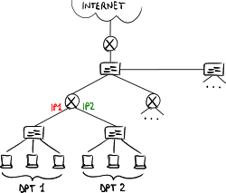 Backbone with IP segmentation.


Where is it better to position routers in a corporate network?
- access: only bridges (typically multilayer switches) connected directly to hosts;
- backbone: two possible solutions exist:
- VLAN segmentation: the whole corporate network is at the data-link layer, and every area (e.g. university department) is assigned a VLAN → mobility is extended to the whole corporate network;
- IP segmentation: each access bridge is connected to a router (typically layer 3 switch), and every area is assigned an IP network → higher network isolation and higher scalability.
Often internal bridges connect all the access routers one to each other and to the exit gateway router;
- edge: a router as the exit gateway toward Internet, usually an L4-7 multilayer switch having features at the transport layer and higher, such as protection (e.g. firewall), quality of service, load balancing, etc.
Example of LAN design
[edit | edit source]
- multilayer switch on the edge:
- with simple routers there would be a different IP network for each floor, to the benefit of mobility between floors;
- as many virtual interfaces are configured on the internal router as VLANs are in the building;
- all the ports towards floor bridges are configured in trunk mode, then every port can accept any VLAN, to the benefit of mobility between floors;
- it is an L4-7 multilayer switch for upper-layer features (in particular security functions);
- traffic between edge routers: an additional VLAN is specifically dedicated to L3 traffic which routers exchange (e.g. OSPF messages, HSRP messages), to split it from normal LAN traffic (otherwise a host may pretend to be a router and sniff traffic between routers);
- Multi-group HSRP (mHSRP): a multilayer switch can be active for some VLANs and stand-by for other ones;
- Per-VLAN Spanning Tree (PVST): a spanning tree protocol instance is active for each VLAN, to optimize paths based on VLANs.
The root bridge must always be the HSRP active router, otherwise some paths are not optimized; - direct link between multilayer switches:
- it provides a direct path for additional L3 traffic between routers;
- it lightens traffic load on floor bridges, which typically are dimensioned to support few traffic;
- ports at the endpoints of the link are configured as L2 ports, to give the possibility even to normal traffic to cross this link in case one of the link to floor bridges fails;
- it is doubled in link aggregation for a greater fault tolerance and to exploit the available bandwidth on both the links (avoiding STP disables one of the two links).
Introduction to Storage Area Networks
Storage architectures
[edit | edit source]A company typically needs to store a lot of data:
- mainframes (historical): data access is centralized on the same machine where they are physically stored;
- client-server model: several clients ask a server machine to retrieve data stored on hard disks;
- peer-to-peer model: data are distributed among all the machines connected one with each other, and every machine can ask every other machine to have some data.
- Comparison
- costs: each machine in a peer-to-peer network does not require a high computing power and a high storage capacity, in contrast to a server having to manage requests from multiple clients at the same time → servers are very expensive;
- scalability: in the peer-to-peer model data can be distributed over an unlimited number of machines, while the computing capacity and the storage capacity of a server are limited;
- robustness: a server is characterized by a high reliability, but a fault is more critical to be solved; machines in a peer-to-peer network instead are more subject to faults because they are low-end and less reliable machines, but software managing the peer-to-peer network, being aware of this weakness, is designed to keep data integrity, by performing for example automatic backups.
- Datacenter
A datacenter is a centralized location where all servers are concentrated, and allows to avoid having too many servers scattered around the company under the control of so many different organizations:
- data access: data may be available, but people needing them may belong to another organization or may not have the required permissions;
- integrity: it is difficult to back up all servers if they are scattered around the company;
- security: it is easy to steal a hard disk from an unprotected server.
DAS
[edit | edit source]In a DAS system, every server has exclusive access to its own hard disk set:
- internal disks: it is not a proper solution for servers because, in case of fault, hard disks have to be physically extracted from the inner of the machine;
- external disks: disks are connected to the server via SCSI; multiple disk sets can be connected in a cascade like a bus architecture.
Disks can be put in a dedicated cabinet called JBOD: the SCSI controller is able to export a virtual drive structure which is different from the one of the physical disks, by aggregating or splitting disk capacities and providing advanced services (e.g. RAID).
The SCSI standard defines a full protocol stack:
- physical interfaces (e.g. cables and connectors): they allow to physically connect hard disks to servers;
- protocols: they allow to perform read and write transactions by directly addressing disk blocks according to the Logical Block Addressing (LBA) schema;
- commands exported to applications: they allow to perform read and write operations by issuing commands like READ, WRITE, FORMAT, etc.
- Advantages
- low latency: it is in the order of milliseconds through a disk and of microseconds through a cache;
- high reliability: the error probability is very low, and the data integrity is always guaranteed;
- wide compatibility: it is widely supported by operating systems and is used by a lot of external devices besides disks.
- Disadvantages
- slow error recovery: since errors rarely occur, error recovery mechanisms are not particularly efficient from the performance point of view;
- centralized access to disks: just the server can access disks → in case the server faults, disks can no longer be accessed;
- scalability limitations: at most 16 devices for a maximum length of 25 meters can be connected in a cascade.
NASes and SANs allow to decouple disks from servers connecting those entities through a network → a disk can be accessed by multiple servers.
NAS
[edit | edit source]
A NAS exports file systems, serving logical files, instead of disk blocks, over the network (usually LAN).
File systems are shared with network clients: both servers and clients connected to the network can access files.
Typical protocols used to export file systems are:
- NFS: popular on UNIX systems;
- CIFS: used by Windows systems;
which work over a TCP/IP network:
| NFS/CIFS |
| TCP |
| IP |
| Ethernet |
- Advantages
- along with the file system, user permissions and access protections (e.g. username and password) can be exported;
- compatibility with network clients: a NAS system has a minimal impact on the existing infrastructure: all operating systems are able to mount a shared disk without additional drivers.
- Disadvantages
- compatibility with applications: the raw disk is invisible to the client: disks can not be formatted or managed at the block level → some applications which need to directly access disk blocks can not work on remote disks: operating systems, database management systems, swap files/partitions;
- the NAS appliance requires enough computational power for user permission management and remapping from file-related requests to block-related requests;
- the protocol stack is not developed for NASes: TCP error-recovery mechanisms may introduce a non-negligible performance overhead.
SAN
[edit | edit source]
A SAN exports physical disks, instead of logical volumes, and allows to address disk blocks according to the LBA schema, just as if the disk was connected directly to the server via SCSI (DAS system).
Clients can access data through servers, which they are connected to via a Wide or Local Area Network. Typically a datacenter follows a three-tier model:
- web server: it is the front-end exposed to clients;
- application/database server: it can mount a shared-disk file system which converts file-related requests by clients to block-related requests to be sent to remote disks via the SAN;
- hard disks: they are often put in JBODs.
SANs can not base exclusively on the classical TCP/IP, since TCP error-recovery mechanisms may introduce a non-negligible performance overhead → some protocols have been developed for SANs aimed to keep as much as possible high speed, low latency and high reliability typical of SCSI:
|
|
|
|
All SAN protocols adopt SCSI as the upper layer in their protocol stacks and work below it → this guarantees compatibility with all the existing SCSI-based applications, with a minimum impact for DAS to SAN migration.
Fibre Channel
[edit | edit source]
The Fibre Channel standard was born from the need to have a reliable support for optical fiber connections between servers and storage disks, and is thought to replace the physical layer of SCSI. Fibre Channel supports high transfer rates: 1 Gbps, 2 Gbps, 4 Gbps, 8 Gbps, 16 Gbps.
Topologies
[edit | edit source]The standard contemplates three possible topologies for SANs:
- point-to-point: direct connection between a server and a JBOD, like in SCSI;
- arbitrated loop: ring topology for reliability purpose;
- switched fabric: multiple servers are connected to multiple JBODs through a fabric, that is a mesh network of bridges.
The switched fabric topology is new in the storage world: SCSI allowed only to connect in a cascade like a bus architecture.
Routing
[edit | edit source]Routing is performed by the Fabric Shortest Path First (FSPF) protocol, very similar to the OSPF protocol in IP networks. No spanning tree protocols are contemplated for rings in topology.
Every port of a Fibre Channel node (server or JBOD) is dynamically assigned a 24-bit address:
| 8 | 16 | 24 |
| Domain ID | Area ID | Port ID |
where the fields are:
- Domain ID field (8 bits): it identifies the bridge which the node is connected to;
- Area ID field (8 bits): it identifies the group of ports which the bridge port, to which the node is connected, belongs to;
- Port ID field (8 bits): it identifies the node port.
Every server is connected to the fabric through an interface called Host Bus Adapter (HBA).
Flow control
[edit | edit source]Fibre Channel enhances SCSI error-recovery mechanisms by introducing a hop-by-hop flow control based on a credit mechanism: each port has an amount of credits, which is decreased whenever a packet is forwarded and is increased whenever an acknowledge is received → if the available amount of credits goes down to 0, the port can not send other packets and has to wait for the next hop to communicate via an acknowledge which it is ready to receive other data into its buffer → this mechanism avoids node buffer congestions and therefore packet losses.
Moreover the credit mechanism allows resource reservation and guarantees in-order delivery of frames: the destination node has not to implement a mechanism for packet re-ordering (like in TCP).
- Issues
- traffic over a link can be blocked for a while due to lack of credits → the maximum number of credits for a port has to be set properly based on the buffer capacity of the port which is at the other endpoint of the link;
- deadlocks may happen in a mesh network with circular dependencies.
Advanced features
[edit | edit source]- Virtual SAN (VSAN): the equivalent of VLANs for SANs;
- link aggregation;
- load balancing;
- virtualization: virtualization features of the SCSI controller can be moved directly to the bridge which the JBOD is connected to.
FCoE
[edit | edit source]| Parts of this page are based on materials from: Wikipedia: the free encyclopedia. |
The Fibre Channel over Ethernet (FCoE) technology allows to encapsulate Fibre Channel frames into Ethernet frames via the FCoE adaptation layer, which replaces the physical layer of Fibre Channel → this allows to use 10 Gigabit Ethernet (or higher speeds) networks while preserving the Fibre Channel protocol.
Before FCoE, datacenters used Ethernet for TCP/IP networks and Fibre Channel for SANs. With FCoE, Fibre Channel becomes another network protocol running on Ethernet, alongside traditional IP traffic: FCoE operates directly above Ethernet in the network protocol stack, in contrast to iSCSI which runs on top of TCP and IP:
- advantage: the server has no longer to have a Fibre Channel-specific HBA interface, but a single NIC interface can provide connectivity both to the SAN and to the Internet → smaller number of cables and bridges, and lower power consumption;
- disadvantage: FCoE is not routable at the IP layer, that is it can not go over the Internet network outside the SAN.
Since, unlike Fibre Channel, the classical Ethernet includes no flow control mechanisms, FCoE required some enhancements to the Ethernet standard to support a priority-based flow control mechanism, to reduce frame loss from congestion.

The basic idea is adopting PAUSE packets from the 802.3x standard for flow control over Ethernet, but the Ethernet channel between two bridges is logically partitioned into lanes (for example, one dedicated to storage traffic and another one dedicated to the normal internet traffic) → the PAUSE packet, instead of blocking the whole traffic over the concerned link, just blocks traffic of a certain lane without affecting traffic of other lanes.
Typically for servers with FCoE technology top-of-the-rack (TOR) switches are preferred to end-of-the-row (EOR) switches used with Fibre Channel, because switches with FCoE technology are less expensive with respect to switches with Fibre Channel technology:
- end-of-the-row switch: there is a single main switch and every server is connected to it through its own cable → longer cables;
- top-of-the-rack switch: on top of each rack there is a switch, and every server is connected to its rack switch, then all rack switches are connected to the main switch → more numerous switches, but shorter cables.
iSCSI
[edit | edit source]
The iSCSI protocol, proposed by Cisco to counteract Fibre Channel hegemony, allows to make a SAN by using the most common network technology, namely TCP/IP: SCSI commands are encapsulated into TCP packets via the iSCSI adaptation layer and cross the SAN over an Ethernet network.
- Advantages
- the server has no longer to have a Fibre Channel-specific HBA interface, but a single NIC interface can provide connectivity both to the SAN and to the Internet → smaller number of cables and bridges, and lower power consumption;
- disks can be reached also by clients via the Internet;
- optical fibers dedicated specifically for SAN connection do not need to be laid.
- Disadvantages
- bridge buffers in the SAN need to be sized so as to minimize packet losses due to buffer overflow and therefore performance overhead due to TCP error-recovery mechanisms;
- the Ethernet technology is not very known in the storage world, where Fibre Channel tools are used to be used → the iSCSI protocol has not been very successful.
FCIP
[edit | edit source]
A datacenter is subject to data loss risk due to natural disasters (like earthquakes, tsunamis, etc.) → in order to improve resiliency (business continuity), the datacenter can entirely be replicated in another location, generally at a distance of some hundred kilometers. The main datacenter and the backup datacenter could communicate one with each other by using Fibre Channel, but connecting them through a simple optical fiber would be too expensive due to the long distance.
The Fibre Channel over IP (FCIP) technology allows geographically distributed SANs to be interconnected by using the existing TCP/IP infrastructure, namely Internet, without making internal devices in datacenters be aware of the presence of the IP network:
- the main datacenter sends a Fibre Channel frame;
- the edge router encapsulates the Fibre Channel frame into a TCP packet, via the FCIP adaptation layer replacing the physical layer of Fibre Channel, then forwards the TCP packet over the Internet network, in a sort of tunnel, up to the other edge router;
- the other edge router extracts the Fibre Channel frame and sends it to the backup datacenter;
- the backup datacenter receives the Fibre Channel frame.
The Fibre Channel frame minimum size, however, exceeds the Ethernet payload size limit, and the overhead for fragmentation would be excessive → Ethernet frames must be extended to about 2.2 KB so that minimum-size Fibre Channel frames can be encapsulated.