
Travel Time Reliability Reference Manual/Printable version
| This is the print version of Travel Time Reliability Reference Manual You won't see this message or any elements not part of the book's content when you print or preview this page. |
The current, editable version of this book is available in Wikibooks, the open-content textbooks collection, at
https://en.wikibooks.org/wiki/Travel_Time_Reliability_Reference_Manual
About the Travel Time Reliability Reference Manual
The Travel Time Reliability Reference Manual is authored and maintained by the Upper Midwest Reliability Resource Center. The main page acts as a table of contents for the manual.
Next Page → Travel Time Reliability Indices
Travel Time Reliability Indices
Reliability Indices
[edit | edit source]Travel Time Index (TTI) - The ratio of a measured travel time during congestion to the time required to make the same trip at free-flow speeds. For example, a TTI of 1.3 indicates a 20-minute free-flow trip required 26 minutes.[1]

Buffer Index (BI) - "The buffer index represents the extra buffer time (or time cushion) that most travelers add to their average travel time when planning trips to ensure on-time arrival. This extra time is added to account for any unexpected delay. The buffer index is expressed as a percentage and its value increases as reliability gets worse. For example, a buffer index of 40 percent means that, for a 20-minute average travel time, a traveler should budget an additional 8 minutes (20 minutes × 40 percent = 8 minutes) to ensure on-time arrival most of the time. In this example, the 8 extra minutes is called the buffer time. The buffer index is computed as the difference between the 95th percentile travel time and average travel time, divided by the average travel time."[2]
"This formulation of the buffer index uses a 95th percentile travel time to represent a near-worst case travel time. Whether expressed as a percentage or in minutes, it represents the extra time a traveler should allow to arrive on-time for 95 percent of all trips. A simple analogy is that a commuter or driver who uses a 95 percent reliability indicator would be late only one weekday per month."[2]

Planning Time Index - "The planning time index represents the total travel time that should be planned when an adequate buffer time is included. The planning time index differs from the buffer index in that it includes typical delay as well as unexpected delay. Thus, the planning time index compares near-worst case travel time to a travel time in light or free-flow traffic. For example, a planning time index of 1.60 means that, for a 15-minute trip in light traffic, the total time that should be planned for the trip is 24 minutes (15 minutes × 1.60 = 24 minutes). The planning time index is useful because it can be directly compared to the travel time index (a measure of average congestion) on similar numeric scales. The planning time index is computed as the 95th percentile travel time divided by the free-flow travel time."[2]

XXth % Travel Time Index - The XXth-percentile travel time index is the ratio of the XXth % travel time to the mean travel time. The XXth-percentile travel time is the travel time at which XX % of travel times are less than or equal to it.

Misery Index (MI) - The misery index measures the amount of delay of the worst trips. For example, the MI may compare the 97.5th percentile travel time to the mean travel time.[3]

On-Time Performance - The percentage of trips which are less than or equal to XX x free-flow travel time, where XX is usually around 1.1-1.3.[3]
Graphical Representation of Travel Time Indices
[edit | edit source]
Previous Page → About the Travel Time Reliability Reference Manual
Travel Time Reliability Reference Manual
References
[edit | edit source]
About NPMRDS
NPMRDS
[edit | edit source]The FHWA acquired a national data set of average travel times for use in performance measurement and to identify transportation improvement areas and monitor their effectiveness.. The National Performance Measure Research Data Set, is provided by HERE North America, LLC (formerly known as Nokia/NAVTEQ). The data set is made available to States and Metropolitan Planning Organizations (MPOs) as a tool for performance measurement. Access can be obtained by emailing e-mail Heretraffic.nhsdata@here.com. [1]
Next Page → Accessing the Data
References
[edit | edit source]
Accessing the Data
Access to NPMRDS Data
[edit | edit source]The data set is made available to States and Metropolitan Planning Organizations (MPOs) as a tool for performance measurement. Access can be obtained by emailing e-mail Heretraffic.nhsdata@here.com. [1]
More information regarding access to the NPMRDS data can be found at http://www.ops.fhwa.dot.gov/freight/freight_analysis/perform_meas/vpds/npmrdsfaqs.htm.
The data typically come out each month in the form of seven compressed .tar files. The files include:
- Documentation
- Canadian and Mexican border data
- Midwest
- Northeast
- South
- US
- West
Next Page → Data Format and Size
References
[edit | edit source]
Data Format and Size
NPMRDS Data Format
[edit | edit source]NPMRDS data comes in two formats. The first is the static file containing the TMC information for all states. This file may be updated from time to time, but is typically static. The remaining files contain the travel time information for each state in the form of comma separated files (CSV). The files are usually between 500MB and 4GB depending on the region, with the Northeast being the largest data set.
A sample Google Earth (.kml) file mapping out the TMCs in Iowa, Minnesota, North Dakota, South Dakota and Wisconsin is available here or on Google Maps here .
TMC Static File Format
| Field Name | Type | Example | Description |
|---|---|---|---|
| TMC | Text | D01N04474 | Traffic Location code in the format of:
CLLDTTTTT Where:
If no data exists for a TMC for an epoch, there will be no entry in the data file for that combination of TMC/day of week/epoch. |
| ADMIN_LEVEL_1 | Text | United States | The Country where the listed Traffic Location Code is located. |
| ADMIN_LEVEL_2 | Text | Illinois | The State / Province where the listed Traffic Location Code is located. |
| ADMIN_LEVEL_3 | Text | DuPage | The County where the listed Traffic Location Code is located. |
| DISTANCE | Float | 3.27285 | The length of the TMC, measured in Miles to five decimal places. |
| ROAD_NUMBER | Text | I-90 | Road Number taken from Location Table. When a Road has both a route number and local name, the route number is placed in the Road Number column and the local name in the Road Name column. |
| ROAD_NAME | Text | S ARCHER AVE | Road Name taken from Location Table. When a Road has both a route number and local name, the route number is placed in the Road Number column and the local name in the Road Name column. |
| LATITUDE | Float | 37.87472 | WGS84 coordinate to five decimal places
Note: latitude & longitudes provided will be for the beginning of the TMC. |
| LONGITUDE | Float | -122.18671 | WGS84 coordinate to five decimal places
Note: latitude & longitudes provided will be for the beginning of the TMC. |
| ROAD_DIRECTION | Text | NORTHBOUND | Road direction represents the direction of travel based on the road sign |
Travel Time File Format
| Field Name | Type | Example | Description |
|---|---|---|---|
| TMC | Text | D01N04474 | Traffic Location code in the format of:
CLLDTTTTT Where:
If no data exists for a TMC for an epoch, there will be no entry in the data file for that combination of TMC/day of week/epoch. |
| DATE | Text | 04022012 | Day Month Year (DDMMYYYY) |
| EPOCH | Integer | 48 | A value from 0 through 287 that defines the 5-minute period the average speed applies (local time), where:
0 = 00:00:00 to 00:04:59 1 = 00:05:00 to 00:09:59 2 = 00:10:00 to 00:14:59 … 287=23:55:00 to 23:59:59 |
| Travel_TIME_ALL_VEHICLES | Integer | 44 | In seconds.
Travel times are calculated as the ratio between the segment length and the average speed on the segment. Average segment speed is determined from a combination of the passenger and freight trucks individual GPS probe speed observations. |
| Travel_TIME_PASSENGER_VEHICLES | Integer | 76 | In seconds.
Travel times are calculated as the ratio between the segment length and the average speed on the segment. Average segment speed is determined from only passenger individual GPS probe speed observations. |
| Travel_TIME_FREIGHT_TRUCKS | Integer | 1 | In seconds.
Travel times are calculated as the ratio between the segment length and the average speed on the segment. Average segment speed is determined from only freight trucks individual GPS probe speed observations. |
Previous Page → Accessing the Data
References
[edit | edit source]- ↑ a b NPMRDS Specification Document (http://www.ops.fhwa.dot.gov/freight/freight_analysis/perform_meas/vpds/npmrdsfaqs.htm)
Data Storage
Data Storage
[edit | edit source]Due to the large size of the NPMRDS data sets, it is not possible to open the CSV files containing travel time data in Microsoft Excel. While Microsoft Access provides the ability to handle slightly larger data sets, MS Access is also limited in the amount of data it can hold (typically around 2 GB). With each month of data containing between 500 MB and 4 GB, depending on the region, it is recommended to use a non file-based relational database. MySQL and PostgreSQL are examples of open source databases which can handle these large data sets.
The data is often stored as two tables, one which holds the static TMC information and the other which holds the speed/travel time data. The two tables can be joined by the TMC id/name which is parameter in both data sets. Details of each data set can be found on the NPMRDS data format page.
Previous Page → Data Format and Size
Next Page → Building Corridors
Building Corridors
Constructing a Segment for Analysis
[edit | edit source]TMCs are segments of the roadway, often between interchanges or major intersections on arterials. The travel time data is reported at the TMC level. These segments range in length from less than a mile to several miles long. In order to build a corridor and calculate the travel time, TMCs must be connected. Each TMC is assigned a location code. Details can be found at Next Page → Data Format.
A Google Earth (.kml) file mapping out the TMCs in Iowa, Minnesota, North Dakota, South Dakota and Wisconsin is available here or on Google Maps here .
Typically, a corridor can be constructed by connecting successive TMCs in the positive or negative direction. The TMC numbers increase with the direction of travel along the positive direction and decrease along the negative direction. For example, a corridor in the positive direction might consiste of 107P04585, followed by 107P04586, 107P04587 and 107P04588 etc. In the negative direction, 107N04588 would be the first TMC, followed by 107N04587, 107N04586, and 107N04585 etc.
Longer corridors, however, can be constructed by simply connecting successive TMCs. When roadways intersect other roadways, the TMC sequence may change. Therefore, viewing TMC points in GIS or other mapping software allows one to see the sequence of TMCs along the desired corridor. The static file containing TMC information, includes the roadway name, direction and latitude and longitude coordinates, allowing the points to be plotted in various programs. The NPMRDS data set also includes a shapefile which can be used to construct corridors in GIS.
One difference in the TMC data provided by INRIX, is that TMC points are defined by a beginning and ending latitude and longitude which typically allows a corridor to be constructed by connecting the ending latitude/longitude of one TMC to the beginning latitude/longitude of another.
Once the order and sequence of TMC points along the corridor is defined, travel times and other metrics can be calculated.
Next Page → Availability of Real-Time Data
Availability of Real-Time Data
NPMRDS Real-Time Data Availability
[edit | edit source]The charts below outline the availability of NPMRDS real-time data on two freeway corridors in January 2012.
The following two graphs show the availability of real-time data by hour of day in January 2012 for the 6-lane urban freeway and the 4-lane inter-regional freeway. The availability of real-time data is higher during daytime hours when vehicle volumes are higher and lower overnight. Overall, the 4-lane inter-regional corridor reported more real-time measurements. Although the urban freeway experiences higher vehicle volumes, the inter-regional freeway likely experiences higher commercial truck volumes, which are often a source of probe data. Another possible factor is the shorter TMC lengths along the urban freeway. The inter-regional freeway is 20 miles long with 4 TMC segments, while the urban freeway is 4 miles long with 6 TMC segments. It's unknown whether there is a correlation between TMC length and availability of real-time data.


The two charts below show the frequency at which varying amounts of real-time data were available along the corridors during January 2012. For example, 100% availability corresponds to all TMCs reporting (4/4 or 6/6 for these two corridors) real-time data during a given time interval, 50% availability to half of TMC segments (2/4 or 3/6) reporting real-time data etc. The frequency at which eac of these occur is plotted along the y-axis. The inter-regional freeway consists of 4 TMCs making up 20.18 miles, the urban freeway 6 TMCs totaling 4.35 miles. The greater number of TMC segments along the urban corridor is one factor leading to the smaller frequencies of availability. However, with fewer real-time data points (as shown in the graphs above), it is expected that the frequencies will also be lower on the urban corridor than the inter-regional.
 6 TMC segments along 4.35 miles of corridor
 4 TMC segments along 20.18 miles of corridor
Previous Page → Building Corridors
Previous Page → Calculating Speeds and Travel Times
Calculating Speeds and Travel Times
Calculating speeds or travel times along a corridor is straightforward given that one has constructed the TMC segments which make up the corridor and that one has a tool by which to access the data. One open source tool for writing the necessary code is Python. Python extensions, such as Psycopg, allow one to access SQL databases which are storing the speed/travel time data.
INRIX and NPMRDS provide either speed or travel time measurements for each TMC for every time interval (1 or 5 minutes). TMC lengths are also reported which allows for easy conversion between speed and travel time. Calculating speeds or travel times along a corridor only requires that these values be aggregated. Python scripting can be used to read from the databases for the necessary TMC segments and desired time periods and loop over the values in order to construct speeds/travel times. These speeds/travel times can then be written to a Comma Value Separated (CSV) file, or inserted into a database table.
Additional add-ons are available for Python which allow 3D graphing capabilities. Below are sample graphs created using the NPMRDS data set and the Matplotlib python library. Blank areas represent points where real-time data did not exist along the entire corridor.
Travel Times for 4-lane Inter-regional Freeway in January 2012

Travel Times for 6-lane Urban Freeway in January 2012

Previous Page → Availability of Real-Time Data
Next Page → Imputing Missing Speed Data
Imputing Missing Speed Data
Unlike INRIX, the NPMRDS data set does not include non real-time travel times or speeds. If real-time measurements do not exist for a given TMC during a given time period, the data point is left blank. In some cases, it may be desirable to impute some of the missing data points based on surrounding real-time data.
The figure below gives an example of imputing a missing data point based on surrounding spatial and temporal data.

Using a sample NPMRDS data set, an imputation was conducted in which missing data points were imputed only if the surrounding spatial and temporal points were all populated with real-time data. The percentage of missing data points which fit this criteria was around 3 percent. More often than not, the missing data points are not anomalies, but are accompanied by other missing points. This makes sense, since missing real-time data is usually the result of a lack of probe vehicles. A lack of real-time data in one TMC segment will likely result in neighboring TMCs to also lack real-time data. Similarly, surrounding temporal points are likely to lack real-time observations when vehicle volumes are low.
Previous Page → Calculating Speeds and Travel Times
Next Page → NPMRDS and INRIX Data Comparison
References
[edit | edit source]
NPMRDS and INRIX Data Comparison
Comparison of INRIX and NPMRDS Data Sets
[edit | edit source]A comparison of speed data between INRIX and NPMRDS for January 2012 on a 4-lane inter-regional and 6-lane urban freeway.
| Urban 6-lane Freeway | INRIX | NPMRDS |
|---|---|---|
| Mean Speed (mph) | 61.05 | 56.90 |
| Standard Deviation (mph) | 4.61 | 6.24 |
| Median Speed (mph) | 61.72 | 58.05 |
| IR 4-lane Freeway | INRIX | NPMRDS |
|---|---|---|
| Mean Speed (mph) | 65.32 | 63.42 |
| Standard Deviation (mph) | 3.69 | 4.83 |
| Median Speed (mph) | 65.49 | 64.00 |
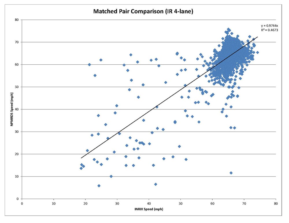
Particularly on the urban freeway, the NPMRDS data reports lower speeds than INRIX with higher variability. The matched pair graphs below reveal a similar trend represented by the linear fit with the intercept set to zero.

Previous Page → Imputing Missing Speed Data
Example Data
Below are graphs and data for an 6-lane urban freeway (I-43/I-894 near Milwaukee) and 4-lane inter-regional (I-94 west of Eau Claire). All data comes from the NPMRDS data set in January 2012.
6-lane urban freeway (4.35 miles) Free flow travel time is based on the 70th percentile travel time
| Reliability Index | Value |
|---|---|
| TTI | 1.01 |
| BI | 0.26 |
| OPT | 94.90 |
| PTI | 1.27 |
| TTI80 | 1.02 |
| MI | 1.40 |
| Travel Time in minutes | |
|---|---|
| Mean | 4.58 |
| Free Flow | 4.55 |
| 95th % | 5.76 |
| 80th % | 4.65 |
| 97.5th % | 6.47 |
4-lane interregional freeway (20.18 miles) Free flow travel time is based on speed limit of 65mph
| Reliability Index | Value |
|---|---|
| TTI | 1.03 |
| BI | 0.06 |
| OPT | 98.40 |
| PTI | 1.09 |
| TTI80 | 1.038 |
| MI | 1.150 |
| Travel Time in minutes | |
|---|---|
| Mean | 19.26 |
| Free Flow | 18.63 |
| 95th % | 20.38 |
| 80th % | 19.33 |
| 97.5th % | 21.42 |
The 3-D graphs below show travel times by day and by hour for each corridor. Visually, one can see the better reliability of the inter-regional corridor over the urban. Blank areas represent points where real-time data did not exist along the entire corridor.
Travel Times for 6-lane Urban Freeway in January 2012
Travel Times for 4-lane Inter-regional Freeway in January 2012
Previous Page → NPMRDS and INRIX Data Comparison
Travel Time Reliability Reference Manual
About INRIX
"As of April 2012, INRIX collects trillions of bytes of information about roadway speeds from nearly 100 million anonymous mobile phones, trucks, delivery vans, and other fleet vehicles equipped with GPS locator devices.[1] Data retrieved from consumer cellular GPS-based devices including the iPhone, Android, BlackBerry and Windows Phone phones, Ford SYNC and Toyota Entune. The data collected is processed in real-time, creating traffic speed information for major freeways, highways and arterials across North America (United States,[2] Canada), as well as much of Europe, South America, and Africa."[3]
See the INRIX Wikipedia Page for more information.
References
[edit | edit source]- ↑ White, Joseph B. (August 14, 2008). "New Services Gather Data In an Effort to Track Current And Future Traffic Jams". The Wall Street Journal. http://online.wsj.com/article/SB120795092324008845.html?mod=googlenews_wsj.
- ↑ "INRIX Flow Coverage". INRIX, Inc.
- ↑ https://en.wikipedia.org/wiki/INRIX
INRIX Data Types
INRIX Speed Data Types
[edit | edit source]INRIX speed data includes a code with each speed observation. This code represents the type of speed: reference, historical or real-time.
Reference speed: based on the typical free flow speed for the segment - related to the speed limit
Historical speed: based on the historical speed data for that particular segment during the same time of day
Real-time speed: based on real-time speed measurements from probe, gps or other real-time measurements
The reference speed is constant across all times and varies only by TMC segment. The historical speed is time dependent and may capture recurring congestion along a segment. INRIX uses reference and historical speeds to fill in gaps in the real-time data. INRIX does not reveal the threshold necessary to provide real-time data, nor does INRIX reveal when reference data is used instead of historical data for filling gaps in real-time data. It appears, however, that reference data is used during the night and other off peak times in order to reduce processing when speeds are likely constant, whereas, historical data is likely used during hours when speeds may vary but no real-time data is available.
Data Type by Year
[edit | edit source]Below are graphs representing the distribution of data types for freeways and arterials in Wisconsin by year. The data does not include all INRIX freeway and arterial coverage in Wisconsin, but a subset. The graphs reveal an increase in the availability of real-time data with time. It is expected that this trend has continued with 2013 and 2014 data.


Data Type by Hour
[edit | edit source]The graph below shows the distribution of real-time data along a 4-lane inter-regional freeway in Wisconsin by hour of the day. Real-time data is most prevalent during daytime hours when more vehicles are present on the roadway.

Next Page → NPMRDS and INRIX Data Comparison
NPMRDS and INRIX Data Comparison
Comparison of INRIX and NPMRDS Data Sets
[edit | edit source]A comparison of speed data between INRIX and NPMRDS for January 2012 on a 4-lane inter-regional and 6-lane urban freeway.
| Urban 6-lane Freeway | INRIX | NPMRDS |
|---|---|---|
| Mean Speed (mph) | 61.05 | 56.90 |
| Standard Deviation (mph) | 4.61 | 6.24 |
| Median Speed (mph) | 61.72 | 58.05 |
| IR 4-lane Freeway | INRIX | NPMRDS |
|---|---|---|
| Mean Speed (mph) | 65.32 | 63.42 |
| Standard Deviation (mph) | 3.69 | 4.83 |
| Median Speed (mph) | 65.49 | 64.00 |
Particularly on the urban freeway, the NPMRDS data reports lower speeds than INRIX with higher variability. The matched pair graphs below reveal a similar trend represented by the linear fit with the intercept set to zero.
Previous Page → Imputing Missing Speed Data
About TICAS
Traffic Information and Condition Analysis System (TICAS) is a powerful traffic data collection and simulation software developed by the Northland Advanced Transportation Systems Research Laboratory (NATARL) at University of Minnesota Duluth. The data source of TICAS comes from the Minnesota freeway detectors which provide traffic flow rates, speed and density data every 30 seconds. The major advantage for using TICAS is it enables user to access corridor-based traffic information, such as travel time and vehicle miles traveled. Those traffic metrics are derived or estimated basing on the traffic raw data archived at Minnesota Traffic Management Center. Data from TICAS can be exported into EXCEL directly, which is convenient for large data collection.[1]
References
[edit | edit source]- ↑ Eil Kwon ,Chongmyung Park. (2012). Development of Freeway Operational Strategies with IRIS-in-Loop Simulation. Available: http://www.lrrb.org/media/reports/201204.pdf. Last accessed 5th May 2014.
Creating Routes
TICAS is a powerful data collection tool for corridor-based traffic study. Travel time and vehicle miles traveled data can be downloaded for the routes created by the users. The database of corridors contains the majority of freeways, trunk highways, and US highways in Minnesota central area, and their directions are specified.
The interface of the tool is user-friendly and straightforward.The procedures for creating routs are stated below.
1. Open TICAS tool, and go to "Data/Performance" tab;
2. Click the button "Edit Route" in the "Route and Times" region;
3. Click " Create Route" tab when a new window named "Route Editor" shows up;
4. Drag down the corridor list, and select a corridor that contains the segment(s) interested;
5. A route will be specified in the right window box if a corridor is selected. For the pins showing on the routes, red pins are actual main lane stations of loop detectors, and pins of other colors represent the exit and enter ramp stations. Find the main lane station that closed to the starting location of the interested segment, right click the pin and select "Section start from here". This helps to specify the starting location of the route;
6. Find the main lane station that closed to the ending location of the interested segment, right click the pin and select "Section end to here". This helps to specify the ending location of the route;
7. Click "Save location" button. Then the new edited route will be listed in the "Route Lists" tab. This route can be extracted directly for data collection use.
Next Page → Primary use in SHRP II
Primary use in SHRP II
TICAS is the software that is primarily used for travel time and vehicle miles traveled (VMT) data collection in Strategic Highway Research Program 2 (SHRP II) Project L38-Pilot Testing of Reliability Data and Analytical Tools. TICAS calculates and provides cumulative travel time with records every 0.1-mile from the specified start point to the end point along the corridor. Data is available in varying time intervals, ranging from 30 seconds to one hour.
For primary test, three corridors were selected, and the routes were created and save in TICAS. The start and end points for the corridors are listed below in Table 1.
Table 1: Corridor Boundaries
| Corridor | From | To | Length (miles) | Number of Stations |
|---|---|---|---|---|
| TH 100 | 77th Street | 57th Avenue | 14.6 | 30 |
| I-94 (I-494 to TH 101) | I-494 | CR 81 | 9.0 | 11 |
| I-94 (Minneapolis to St. Paul) | Plymouth Avenue | Mounds Boulevard | 12.8 | 29 |
The team downloaded data from January 2006 through December 2012 for each corridor. Downloading the traffic data was a time consuming effort due to the fact that the TICAS software is only capable of calculating two months of data per query. In addition, when downloading the data for TH 100, TICAS would tend to quit working if more than two weeks of data were selected at one time, due to the large number of stations along the corridor. If days with no travel time or VMT data available were selected when using TICAS, an “Error in evaluation” message would appear. When this occurred, each individual day had to be checked to determine which days were missing data. After recognizing that, in general, the only days with missing data were the first Saturday and Sunday of November each year (on occasion, the last weekend of October was missing data), the search was narrowed down fairly quickly and the days with missing data were simply not selected in TICAS.
Table 2: Days with Missing TICAS Data
| Year | Days with Missing Data |
|---|---|
| 2006 | October 28th-29th |
| 2007 | November 3rd -4th |
| 2008 | November 1th -2th |
| 2009 | October 31st-November 1st |
| 2010 | November 6th -7th |
| 2011 | November 5th -6th |
| 2012 | November 3rd -4th |
For the further extension of the SHRP II Project L38, the team also downloaded the travel time and VMT data from TICAS on I-35E and TH 13. Instead of performing analysis with seven-year data, only data in year 2012 was downloaded.
In summary, TICAS is a powerful software that could provide corridor-based traffic metrics like travel time and VMT. The data can be collected in every 30 seconds and can be specified in every 0.1 mile. However, there are some limitations when using TICAS. Firstly, downloading the traffic data with multiple years was a time consuming effort due to the fact that the TICAS software is only capable of calculating two months of data per query. Secondly, there is no button like "Select All" which enable user to download the data in large number of days. For example, if user needs to download certain traffic data for a whole year in 2012, TICAS does not allow selecting 366 days in 2012 directly, but select one by one for 366 times. Thirdly, TICAS cannot identify the specific date with error traffic data, but only give user a “Error in evaluation” message. When this occurs, each individual day has to be checked to determine which days are missing data.
Previous Page → Creating Routes
Next Page → Travel Time Reliability Reference Manual
About SHRP II
Strategic Highway Research Program 2 (SHRP II)
[edit | edit source]
"Congress authorized the second Strategic Highway Research Program (SHRP 2) in 2005 to investigate the underlying causes of highway crashes and congestion in a short-term program of focused research. To carry out that investigation, SHRP 2 targets goals in four interrelated focus areas: Safety: Significantly improve highway safety by understanding driving behavior in a study of unprecedented scale. Renewal: Develop design and construction methods that cause minimal disruption and produce long-lived facilities to renew the aging highway infrastructure. Reliability: Reduce congestion and improve travel time reliability through incident management, response, and mitigation. Capacity: Integrate mobility, economic, environmental, and community needs into the planning and design of new transportation capacity."[1]
"SHRP 2 is being conducted under a memorandum of understanding among the American Association of State Highway and Transportation Officials, the Federal Highway Administration, and the National Research Council. The multiyear program (five years of funding, nine years to complete) began work in March 2006. SHRP 2 is guided by an oversight committee and four technical coordinating committees, one in each of the four focus areas. More targeted task groups provide assistance in areas requiring specific technical expertise, including preparation of requests for proposals and review of proposals."[1]
References
[edit | edit source]
TTRMS Tool
The SHRP 2 reliability data and analytical tools are intended to address travel time variability in one of three ways:
1) Establish monitoring systems to identify sources of unreliable travel times;
2) Identify potential solutions to cost-effectively improve reliability;
3) Incorporate consideration of travel time reliability into transportation agencies’ planning and programming framework.
This technical memorandum documents the development of a travel time reliability monitoring system (TTRMS) for the Minnesota pilot site. The development of this system followed the guidelines of the SHRP 2 Project L02 guidebook: Guide to Establishing Monitoring Programs for Travel Time Reliability (September 10, 2012).
This document details the data sources used in the development of the TTRMS for the Minnesota Pilot site. This includes:
• Travel time and traffic data;
• TTRMS database development;
• TTRMS analysis tool
Travel time and other traffic data can be accessed from TICAS. Comparing with the MnDOT data extraction tools, TICAS performs a number of additional calculations using the data from the detector stations to produce the travel time and VMT information. The TTRMS database is configured using a macro-enabled Microsoft Excel spreadsheet. This software package was identified to be the most user-friendly and data compatible for the variety of data sources under consideration. The macros that were developed for the database application assist in the organization of the various data sources to construct the database. This section describes how these features operate and how the various data sources are linked in the database.
A series of refinements were made throughout the development of the database. For example, the database allows users to specify corridor length if a shorter segment of the overall corridor is to be analyzed. In addition, it is capable of accommodating a variety of observation time bins (e.g. 1, 2, 3, 5, 10, or 15-minutes), provided the traffic data is in the corresponding format. These refinements are expected to be used to their full capabilities in later stages of this study and the findings documented in future memoranda.
Input Data Processing
This section explains how the TTRMS interprets each data source and configures it to a standardized format allowing the data to be combined in the TTRMS database.
Traffic Data
The traffic data downloaded using TICAS determined the maximum corridor length and the analysis time interval. The start and end point was chosen based on the detector stations, and travel time and VMT output data is provided in 0.1-mile increments.
Weather Data
A process in the database reformatted the weather data into the appropriate length time intervals as determined by the traffic data. When the time interval from the raw weather data was greater than five minutes, the missing intervals were assigned the conditions of the previous bin until another record was available. For example in a five-minute system, if the source data interval was from 13:05 to 13:20, the travel time records for the 13:10 and 13:15 bins would be assigned the 13:05 weather record. Conversely, when multiple records were available in a single five-minute bin, the most severe weather condition was chosen to represent the bin. Table 1 ranks the precipitation type and intensity by descending order.
Table 1 Precipitation Type and Intensity Hierarchy
| Precipitation Type | Precipitation Intensity |
|---|---|
| Snow | Heavy |
| Frozen | Moderate |
| Rain | Slight |
| Other | None |
| None |
Crash and Incident Data
Crashes are motor vehicle collisions with other vehicles or fixed objects that result in over $1,000 of property damage or personal injury. These events are recorded by law enforcement personnel, and crash records are compiled in the Minnesota Department of Public Safety (DPS) database. Incidents are any other non-recurring disruption to the highway that has the potential to affect capacity and throughput. These situations can include stalled vehicles, medical emergencies, or animals and debris that are on the roadway.These are frequently used to perform safety reviews on highways by computing historical crash rates to identify high crash locations.For crash data, the duration was added to the start time to determine when the crash had cleared. If the crash spanned multiple time intervals, all of the time bins contained in the duration were assigned with the crash details. Similar to the weather data, if crashes overlapped, the “worst” crash (based on severity) was selected to populate the affected time bins. A similar process was used for the incident data, with “Incident Impact” used as the hierarchy variable.
Event Data
Events defined in the TTRMS tool are sports games, concerts, state fairs that have significant impacts on traffic. When an event was taking place, all time bins in the arrival and departure windows were marked with the name of the event type. Each event type was assigned name, such as “Twins_A” (for arrival) or “Vikings_D” (for departure). For instances with multiple events taking place, the names of events were combined to reference both events. For example, if a Twins game arrival overlapped a Vikings game arrival, the event would be categorized as “Twins_A_Vikings_A”.
Road Work
Road work is defined as any agency activity to maintain or improve the roadway that may result in impacts to capacity. This may include short-term activities such as guardrail, sign, or lighting repair as well as more significant, long term construction actions.Road work records were applied to the TTRMS records using a similar protocol as the crash, incident, and event conditions. The input data included start time, end time, and impact attributes. All travel time records during the periods that the road work was active were assigned with the impact category.
Next Page → Surface Plots of non-recurring events
Surface Plots of non-recurring events
TTRMS analysis tool provides numerous important surface plots that display individual records throughout an entire year for each corridor. This makes the plots more accurate and easier to compare with surface plots from other years and corridors. For all of the surface plots shown in this section, each day of the year is shown across the x-axis from left to right. The time of day is shown on the y-axis from bottom to top and is split into five-minute time intervals.
Surface plots were prepared for all of the data elements included in the travel time reliability monitoring system (TTRMS) database. These can broadly be categorized in two groups: one is the traffic data, which is continuous and includes the aggregate measures of vehicle miles travelled (VMT) and travel time. The other is the non-recurring conditions data. These records are not necessarily continuous as there are times when none of these conditions are present on the corridor. The non-recurring conditions include:
• Weather
• Crash
• Incident
• Road Work
• Event
Figure 1 and Figure 2 are examples of the surface plot for the crashes and incidents in 2012 along the I-94 Westbound from I-494 to TH 101. Crash and incident information was gathered from three different sources, which include:
• Minnesota State Patrol Computer Aided Dispatch (CAD) data
• MnDOT’s Dynamic Message Sign (DMS) logs
• Minnesota Department of Public Safety (DPS) crash records.
Crash plots are color coded by crash severity. Incident plots are color coded by impact to roadway capacity.

Figure 1: 2012 WB I-94 Crash Surface Plot

Figure 2: 2012 WB I-94 incident Surface Plot
Figure 3 is an weather surface plot example that shows the weather data collected at the Weather Underground site near the I-94 study corridor in 2012. The colors in the legend represent the precipitation type.

Figure 3: 2012 WB I-94 Weather Surface Plot
Figure 4 is an event surface plot example. The majority of the events considered in this analysis take place during or after the p.m. peak period. Therefore, events have a greater impact on the corridors where the traffic volume is highest during the p.m. peak period.

Figure 4: 2012 WB I-94 Event Surface Plot
Next Page → Surface Plots of travel time and VMT
Surface Plots of travel time and VMT
TTRMS tool is able to provide surface plots of travel time and VMT as well. Those plots can give user a visual view of the reliability of travel by time of day and day of the year. Instead of displaying travel time on the plots, TTRMS analysis tool uses travel time index (TTI). The travel time index is the ratio of the observed travel time divided by the speed limit (free-flow) travel time. This allows for an easier comparison between each of the corridors regardless of length or free-flow speed. The following thresholds were used for the travel time surface plots:
• Speed limit travel time
• The 45 miles per hour (mph) travel time. This threshold was chosen because MnDOT defines congestion as 45 mph or less.
• 1.5-2.0 times the TTI
• 2.0-2.5 times the TTI
• 2.5-3.0 times the TTI
• 3.0-3.5 times the TTI
• 3.5-4.0 times the TTI
• Greater than 4.0 times the TTI
Figure 1 is a example of TTI surface plot along I-94 Westbound from I-494 to TH 101 in 2012. The colors in the legends represent different TTI levels. The plots can automatically updated by different free-flow travel time input.

Figure 1: 2012 WB I-94 Travel Time Surface Plot
Figure 2 is a example of vehicle miles traveled (VMT) surface plot along I-94 Westbound from I-494 to TH 101 in 2012. In this plot, each five-minute observation is displayed as a unique value. Seven VMT bins with increments of 750 vehicle-miles were selected for the VMT surface. In addition, the plot and bins can be updated by entering different "base VMT" to the TTRMS analysis tool.

Figure 2: 2012 WB I-94 VMT Surface Plot
Previous Page → Surface Plots of non-recurring events
Next Page → Other travel time reliability plots
Other travel time reliability plots
TTRMS analysis tool can also provide user the observed frequency of each of the non-recurring factors. Figure 1 is an example of observation along I-94 Westbound from downtown St. Paul to downtown Minneapolis. This represents the number of fifteen-minute intervals throughout the year that have these factors present in the database. In this example, 60 percent of the time intervals do not have any non-recurring factors present, i.e. normal conditions. The intervals with a single factor observed, such as weather, crash, incident, event or roadwork, range from one percent to ten percent of the intervals. Time intervals with two or more factors present are shown in the combinations category and were observed in nine percent of the time intervals in 2012.

Figure 1: 2012 WB I-94 Observation Pie Chart
Figure 2 shows the delay experienced during each of the regimes. To calculate this, the average delay for each time period (observed travel time minus free-flow travel time) is multiplied by the number of users during that time period. All of the time periods are then separated by regime to establish the proportion of delay experienced under each condition. Comparing this chart to Figure 1 shows that a disproportionate amount of the delay is experienced during times with non-recurring factors present, indicating that these factors contribute to increased delay on the corridor.

Figure 2: 2012 WB I-94 Delay Pie Chart
However, there is an argument that a portion of the event delay was likely due to normal delay but not caused by the specific event. For example, 15 percent of crash delay is derived in the example stated above. The right interpretation of the number is that 15 percent of delay is observed during crash time. It cannot be explained as 15 percent of delay is caused by crash because normal delay is included in the 15 percent. TTRMS tool can also provide an adjusted delay pie chart that represents the particular event delay. The basic methodology TTRMS tool applied is to subtract the average normal delay in the specific time when events occurred from the observed delay during events. For example, if a crash lasted for 30 minutes, and the observed corridor delay is 1,000 hours, and the average normal congestion delay is 400 hours, the adjusted delay for this particular crash is 600 hours (1,000 hr- 600 hr) rather than 1,000. However, if a crash lasted for 30 minutes, and the observed corridor delay is 1,000 hours, and the average normal congestion delay is 1,400 hours, the adjusted delay for this particular crash is 0, which indicates that the specific crash does not cause delay at all. Figure 3 shows the adjusted delay pie chart. Comparing with Figure 2 that displays the observed delay pie chart, all of portions for non-recurring events decrease. This chart is more accurate if user would like to analyze the association between the delay and specific types of events.

Figure 3: 2012 WB I-94 Adjusted Delay Pie Chart
Figure 4 shows the delays caused by non-recurring events only along I-94 Westbound from downtown St. Paul to downtown Minneapolis. This chart shows the same things with Figure 3 except excluding the normal congestion delay.

Figure 4: 2012 WB I-94 Adjusted Delay Pie Chart for non-recurring events
Previous Page → Surface Plots of travel time and VMT
Next Page → Travel Time Reliability Reference Manual