Statistical Analysis: an Introduction using R/Chapter 2
Data is the life blood of statistical analysis. A recurring theme in this book is that most analysis consists of constructing sensible statistical models to explain the data that has been observed. This requires a clear understanding of the data and where it came from. It is therefore important to know the different types of data that are likely to be encountered. Thus in this chapter we focus on different types of data, including simple ways in which they can be examined, and how data can organised into coherent datasets.
R topics in Chapter 2
The R examples used in this chapter are intended to introduce you to the nuts and bolts of R, so may seem dry or even overly technical compared to the rest of the book. However, the topics introduced here are essential to understand how to use R and it is particularly important to understand them. They assume that you are comfortable with the concepts of assignment (i.e. storing objects) and functions, as detailed previously.
Variables
[edit | edit source]The simplest sort of data is just a collection of measurements, each measurement being a single "data point". In statistics, a collection of single measurements of the same sort is commonly known as a variable, and these are often given a name[1]. Variables usually have a reasonable amount of background context associated with them: what the measurements represent, why and how they were collected, whether there are any known omissions or exceptional points, and so forth. Knowing or finding out this associated information is an essential part of any analysis, along with examination of the variables (e.g. by plotting or other means).
Single variables in R
[edit | edit source]Vectors
TRUE or FALSE[2]). In this topic we will use some example vectors provided by the "datasets" package, containing data on States of the USA (see ?state).
R is an inherently vector-based program; in fact the numbers we have been using in previous calculations are just treated as vectors with a single element. This means that most basic functions in R will behave sensibly when given a vector as a argument, as shown below.state.area #a NUMERIC vector giving the area of US states, in square miles
state.name #a CHARACTER vector (note the quote marks) of state names
sq.km <- state.area*2.59 #Arithmetic works on numeric vectors, e.g. convert sq miles to sq km
sq.km #... the new vector has the calculation applied to each element in turn
sqrt(sq.km) #Many mathematical functions also apply to each element in turn
range(state.area) #But some functions return different length vectors (here, just the max & min).
length(state.area) #and some, like this useful one, just return a single value.[1] 51609 589757 113909 53104 158693 104247 5009 2057 58560 58876 6450 83557 56400
[14] 36291 56290 82264 40395 48523 33215 10577 8257 58216 84068 47716 69686 147138 [27] 77227 110540 9304 7836 121666 49576 52586 70665 41222 69919 96981 45333 1214 [40] 31055 77047 42244 267339 84916 9609 40815 68192 24181 56154 97914 > state.name #a CHARACTER vector (note the quote marks) of state names
[1] "Alabama"            "Alaska"             "Arizona"            "Arkansas"
[5] "California"         "Colorado"           "Connecticut"        "Delaware"
[9] "Florida"            "Georgia"            "Hawaii"             "Idaho"
[13] "Illinois" "Indiana" "Iowa" "Kansas" [17] "Kentucky" "Louisiana" "Maine" "Maryland" [21] "Massachusetts" "Michigan" "Minnesota" "Mississippi" [25] "Missouri" "Montana" "Nebraska" "Nevada" [29] "New Hampshire" "New Jersey" "New Mexico" "New York" [33] "North Carolina" "North Dakota" "Ohio" "Oklahoma" [37] "Oregon" "Pennsylvania" "The smallest state" "South Carolina" [41] "South Dakota" "Tennessee" "Texas" "Utah" [45] "Vermont" "Virginia" "Washington" "West Virginia" [49] "Wisconsin" "Wyoming" > sq.km <- state.area*2.59 #Standard arithmatic works on numeric vectors, e.g. convert sq miles to sq km > sq.km #... giving another vector with the calculation performed on each element in turn
[1]  133667.31 1527470.63  295024.31  137539.36  411014.87  269999.73   12973.31    5327.63
[9]  151670.40  152488.84   16705.50  216412.63  146076.00   93993.69  145791.10  213063.76
[17] 104623.05 125674.57 86026.85 27394.43 21385.63 150779.44 217736.12 123584.44 [25] 180486.74 381087.42 200017.93 286298.60 24097.36 20295.24 315114.94 128401.84 [33] 136197.74 183022.35 106764.98 181090.21 251180.79 117412.47 3144.26 80432.45 [41] 199551.73 109411.96 692408.01 219932.44 24887.31 105710.85 176617.28 62628.79 [49] 145438.86 253597.26 > sqrt(sq.km) #Many mathematical functions also apply to each element in turn
[1]  365.60540 1235.90883  543.16140  370.86299  641.10441  519.61498  113.90044   72.99062
[9]  389.44884  390.49819  129.24976  465.20171  382.19890  306.58390  381.82601  461.58830
[17] 323.45487 354.50609 293.30334 165.51263 146.23826 388.30328 466.62203 351.54579 [25] 424.83731 617.32278 447.23364 535.06878 155.23324 142.46136 561.35100 358.33202 [33] 369.04978 427.81111 326.74911 425.54695 501.17940 342.65503 56.07370 283.60615 [41] 446.71213 330.77479 832.11058 468.96955 157.75712 325.13205 420.25859 250.25745 [49] 381.36447 503.58441 > range(state.area) #But some functions return different length vectors (here, just the max & min). [1] 1214 589757 > length(state.area) #and some, like this useful one, just return a single value. [1] 50
c(), so named because it concatenates objects together. However, if you wish to create vectors consisting of regular sequences of numbers (e.g. 2,4,6,8,10,12, or 1,1,2,2,1,1,2,2) there are several alternative functions you can use, including seq(), rep(), and the : operator.c("one", "two", "three", "pi") #Make a character vector
c(1,2,3,pi) #Make a numeric vector
seq(1,3) #Create a sequence of numbers
1:3 #A shortcut for the same thing (but less flexible)
i <- 1:3 #You can store a vector
i
i <- c(i,pi) #To add more elements, you must assign again, e.g. using c()
i
i <- c(i, "text") #A vector cannot contain different data types, so ...
i #... R converts all elements to the same type
i+1 #The numbers are now strings of text: arithmetic is impossible
rep(1, 10) #The "rep" function repeats its first argument
rep(3:1,10) #The first argument can also be a vector
huge.vector <- 0:(10^7) #R can easily cope with very big vectors
#huge.vector #VERY BAD IDEA TO UNCOMMENT THIS, unless you want to print out 10 million numbers
rm(huge.vector) #"rm" removes objects. Deleting huge unused objects is sensible[1] "one" "two" "three" "pi" > c(1,2,3,pi) #Make a numeric vector [1] 1.000000 2.000000 3.000000 3.141593 > seq(1,3) #Create a sequence of numbers [1] 1 2 3 > 1:3 #A shortcut for the same thing (but less flexible) [1] 1 2 3 > i <- 1:3 #You can store a vector > i [1] 1 2 3 > i <- c(i,pi) #To add more elements, you must assign again, e.g. using c() > i [1] 1.000000 2.000000 3.000000 3.141593 > i <- c(i, "text") #A vector cannot contain different data types, so ... > i #... R converts all elements to the same type [1] "1" "2" "3" "3.14159265358979" "text" > i+1 #The numbers are now strings of text: arithmetic is impossible Error in i + 1 : non-numeric argument to binary operator > rep(1, 10) #The "rep" function repeats its first argument
[1] 1 1 1 1 1 1 1 1 1 1
> rep(3:1,10) #The first argument can also be a vector
[1] 3 2 1 3 2 1 3 2 1 3 2 1 3 2 1 3 2 1 3 2 1 3 2 1 3 2 1 3 2 1
> huge.vector <- 0:(10^7) #R can easily cope with very big vectors > #huge.vector #VERY BAD IDEA TO UNCOMMENT THIS, unless you want to print out 10 million numbers > rm(huge.vector) #"rm" removes objects. Deleting huge unused objects is sensible
Accessing elements of vectors
[] (i.e. square brackets). If these square brackets contain
- A positive number or numbers, then this has the effect of picking those particular elements of the vector
- A negative number or numbers, then this has the effect of picking the whole vector except those elements
- A logical vector, then each element of the logical vector indicates whether to pick (if TRUE) or not (if FALSE) the equivalent element of the original vector[3].
min(state.area)    #This gives the area of the smallest US state...
which.min(state.area) #... this shows which element it is (the 39th as it happens)
state.name[39]     #You can obtain individual elements by using square brackets
state.name[39] <- "THE SMALLEST STATE" #You can replace elements using [] too
state.name       #The 39th name ("Rhode Island") should now have been changed
state.name[1:10]    #This returns a new vector consisting of only the first 10 states
state.name[-(1:10)]  #Using negative numbers gives everything but the first 10 states
state.name[c(1,2,2,1)] #You can also obtain the same element multiple times
###Logical vectors are a little more complicated to get your head round
state.area < 10000       #A LOGICAL vector, identifying which states are small
state.name[state.area < 10000] #So this can be used to select the names of the small states[1] 1214 > which.min(state.area) #... this shows which element it is (the 39th as it happens) [1] 39 > state.name[39] #You can obtain individual elements by using square brackets [1] "Rhode Island" > state.name[39] <- "The smallest state" #You can replace elements using [] too > state.name #The 39th name ("Rhode Island") should now have been changed
[1] "Alabama"      "Alaska"       "Arizona"      "Arkansas"
[5] "California"     "Colorado"      "Connecticut"    "Delaware"
[9] "Florida"      "Georgia"      "Hawaii"       "Idaho"
[13] "Illinois" "Indiana" "Iowa" "Kansas" [17] "Kentucky" "Louisiana" "Maine" "Maryland" [21] "Massachusetts" "Michigan" "Minnesota" "Mississippi" [25] "Missouri" "Montana" "Nebraska" "Nevada" [29] "New Hampshire" "New Jersey" "New Mexico" "New York" [33] "North Carolina" "North Dakota" "Ohio" "Oklahoma" [37] "Oregon" "Pennsylvania" "THE SMALLEST STATE" "South Carolina" [41] "South Dakota" "Tennessee" "Texas" "Utah" [45] "Vermont" "Virginia" "Washington" "West Virginia" [49] "Wisconsin" "Wyoming" > state.name[1:10] #This returns a new vector consisting of only the first 10 states
[1] "Alabama"   "Alaska"   "Arizona"   "Arkansas"  "California" "Colorado"
[7] "Connecticut" "Delaware"  "Florida"   "Georgia"
> state.name[-(1:10)] #Using negative numbers gives everything but the first 10 states
[1] "Hawaii"       "Idaho"       "Illinois"      "Indiana"
[5] "Iowa"        "Kansas"       "Kentucky"      "Louisiana"
[9] "Maine"       "Maryland"      "Massachusetts"   "Michigan"
[13] "Minnesota" "Mississippi" "Missouri" "Montana" [17] "Nebraska" "Nevada" "New Hampshire" "New Jersey" [21] "New Mexico" "New York" "North Carolina" "North Dakota" [25] "Ohio" "Oklahoma" "Oregon" "Pennsylvania" [29] "THE SMALLEST STATE" "South Carolina" "South Dakota" "Tennessee" [33] "Texas" "Utah" "Vermont" "Virginia" [37] "Washington" "West Virginia" "Wisconsin" "Wyoming" > state.name[c(1,2,2,1)] #You can also obtain the same element multiple times [1] "Alabama" "Alaska" "Alaska" "Alabama" > ###Logical vectors are a little more complicated to get your head round > state.area < 10000 #A LOGICAL vector, identifying which states are small
[1] FALSE FALSE FALSE FALSE FALSE FALSE TRUE TRUE FALSE FALSE TRUE FALSE FALSE FALSE FALSE
[16] FALSE FALSE FALSE FALSE FALSE TRUE FALSE FALSE FALSE FALSE FALSE FALSE FALSE TRUE TRUE [31] FALSE FALSE FALSE FALSE FALSE FALSE FALSE FALSE TRUE FALSE FALSE FALSE FALSE FALSE TRUE [46] FALSE FALSE FALSE FALSE FALSE > state.name[state.area < 10000] #So this can be used to select the names of the small states [1] "Connecticut" "Delaware" "Hawaii" "Massachusetts" [5] "New Hampshire" "New Jersey" "THE SMALLEST STATE" "Vermont"
[] operator can be used to access just a single element of a vector, it is particularly useful for accessing a number of elements at once. Another operator, the double square-bracket ([[) exists for specifically accessing a single element. While not particularly useful for vectors, it comes into its own for #Lists and #Data frames.
Logical operations
<) to produce a logical vector, which could then be used to select elements less than a certain value. This type of logical operation is very useful thing to be able to do. As well as <, there are a handful of other comparison operators. Here is the full set (See ?Comparison for more details)
<(less than) and<=(less than or equal to)>(greater than) and>=(greater than or equal to)==(equal to[4]) and!=(not equal to)
Even more flexibility can be gained by combining logical vectors using and, or, and not. For example, we might want to identify which US states have an area less than 10 000 or greater than 100 000 square miles, or to identify which have an area greater than 100 000 square miles and which have a short name. The code below shows how can be used to do this, using the following R symbols:
&("and")|("or")!("not")
When using logical vectors, the following functions are particularly useful, as illustrated below
which()identifies which elements of a logical vector areTRUEsum()can be used to give the number of elements of a logical vector which areTRUE. This is becausesum()forces its input to be converted to numbers, and if TRUE and FALSE are converted to numbers, they take the values 1 and 0 respectively.ifelse()returns different values depending on whether each element of a logical vector is TRUE or FALSE. Specifically, a command such asifelse(aLogicalVector, vectorT, vectorF)takesaLogicalVectorand returns, for each element that isTRUE, the corresponding element fromvectorT, and for each element that isFALSE, the corresponding element fromvectorF. An extra elaboration is that ifvectorTorvectorFare shorter thanaLogicalVectorthey are extended by duplication to the correct length.
### In these examples, we'll reuse the American states data, especially the state names
### To remind yourself of them, you might want to look at the vector "state.names"

nchar(state.name)       # nchar() returns the number of characters in strings of text ...
nchar(state.name) <= 6  #so this indicates which states have names of 6 letters or fewer
ShortName <- nchar(state.name) <= 6         #store this logical vector for future use
sum(ShortName)          #With a logical vector, sum() tells us how many are TRUE (11 here)
which(ShortName)        #These are the positions of the 11 elements which have short names
state.name[ShortName]   #Use the index operator [] on the original vector to get the names
state.abb[ShortName]    #Or even on other vectors (e.g. the 2 letter state abbreviations)

isSmall <- state.area < 10000  #Store a logical vector indicating states <10000 sq. miles
isHuge  <- state.area > 100000 #And another for states >100000 square miles in area
sum(isSmall)                   #there are 8 "small" states
sum(isHuge)                    #coincidentally, there are also 8 "huge" states

state.name[isSmall | isHuge]   # | means OR. So these are states which are small OR huge
state.name[isHuge & ShortName] # & means AND. So these are huge AND with a short name
state.name[isHuge & !ShortName]# ! means NOT. So these are huge and with a longer name

### Examples of ifelse() ###

ifelse(ShortName, state.name, state.abb) #mix short names with abbreviations for long ones
# (think of this as "*if* ShortName is TRUE then use state.name *else* use state.abb)

### Many functions in R increase input vectors to the correct size by duplication ###
ifelse(ShortName, state.name, "tooBIG")   #A silly example: the 3rd argument is duplicated
size <- ifelse(isSmall, "small", "large") #A more useful example, for both 2nd & 3rd args
size                                      #might be useful as an indicator variable?
ifelse(size=="large", ifelse(isHuge, "huge", "medium"), "small") #A more complex example> ### In these examples, we'll reuse the American states data, especially the state names > ### To remind yourself of them, you might want to look at the vector "state.names" > > nchar(state.name) # nchar() returns the number of characters in strings of text ... [1] 7 6 7 8 10 8 11 8 7 7 6 5 8 7 4 6 8 9 5 8 13 8 9 11 8 7 8 6 13 [30] 10 10 8 14 12 4 8 6 12 12 14 12 9 5 4 7 8 10 13 9 7 > nchar(state.name) <= 6 #so this indicates which states have names of 6 letters or fewer [1] FALSE TRUE FALSE FALSE FALSE FALSE FALSE FALSE FALSE FALSE TRUE TRUE FALSE FALSE [15] TRUE TRUE FALSE FALSE TRUE FALSE FALSE FALSE FALSE FALSE FALSE FALSE FALSE TRUE [29] FALSE FALSE FALSE FALSE FALSE FALSE TRUE FALSE TRUE FALSE FALSE FALSE FALSE FALSE [43] TRUE TRUE FALSE FALSE FALSE FALSE FALSE FALSE > ShortName <- nchar(state.name) <= 6 #store this logical vector for future use > sum(ShortName) #With a logical vector, sum() tells us how many are TRUE (11 here) [1] 11 > which(ShortName) #These are the positions of the 11 elements which have short names [1] 2 11 12 15 16 19 28 35 37 43 44 > state.name[ShortName] #Use the index operator [] on the original vector to get the names [1] "Alaska" "Hawaii" "Idaho" "Iowa" "Kansas" "Maine" "Nevada" "Ohio" "Oregon" [10] "Texas" "Utah" > state.abb[ShortName] #Or even on other vectors (e.g. the 2 letter state abbreviations) [1] "AK" "HI" "ID" "IA" "KS" "ME" "NV" "OH" "OR" "TX" "UT" > > isSmall <- state.area < 10000 #Store a logical vector indicating states <10000 sq. miles > isHuge <- state.area > 100000 #And another for states >100000 square miles in area > sum(isSmall) #there are 8 "small" states [1] 8 > sum(isHuge) #coincidentally, there are also 8 "huge" states [1] 8 > > state.name[isSmall | isHuge] # | means OR. So these are states which are small OR huge [1] "Alaska" "Arizona" "California" "Colorado" "Connecticut" [6] "Delaware" "Hawaii" "Massachusetts" "Montana" "Nevada" [11] "New Hampshire" "New Jersey" "New Mexico" "Rhode Island" "Texas" [16] "Vermont" > state.name[isHuge & ShortName] # & means AND. So these are huge AND with a short name [1] "Alaska" "Nevada" "Texas" > state.name[isHuge & !ShortName]# ! means NOT. So these are huge and with a longer name [1] "Arizona" "California" "Colorado" "Montana" "New Mexico" > > ### Examples of ifelse() ### > > ifelse(ShortName, state.name, state.abb) #mix short names with abbreviations for long ones [1] "AL" "Alaska" "AZ" "AR" "CA" "CO" "CT" "DE" "FL" [10] "GA" "Hawaii" "Idaho" "IL" "IN" "Iowa" "Kansas" "KY" "LA" [19] "Maine" "MD" "MA" "MI" "MN" "MS" "MO" "MT" "NE" [28] "Nevada" "NH" "NJ" "NM" "NY" "NC" "ND" "Ohio" "OK" [37] "Oregon" "PA" "RI" "SC" "SD" "TN" "Texas" "Utah" "VT" [46] "VA" "WA" "WV" "WI" "WY" > # (think of this as "*if* ShortName is TRUE then use state.name *else* use state.abb) > > ### Many functions in R increase input vectors to the correct size by duplication ### > ifelse(ShortName, state.name, "tooBIG") #A silly example: the 3rd argument is duplicated [1] "tooBIG" "Alaska" "tooBIG" "tooBIG" "tooBIG" "tooBIG" "tooBIG" "tooBIG" "tooBIG" [10] "tooBIG" "Hawaii" "Idaho" "tooBIG" "tooBIG" "Iowa" "Kansas" "tooBIG" "tooBIG" [19] "Maine" "tooBIG" "tooBIG" "tooBIG" "tooBIG" "tooBIG" "tooBIG" "tooBIG" "tooBIG" [28] "Nevada" "tooBIG" "tooBIG" "tooBIG" "tooBIG" "tooBIG" "tooBIG" "Ohio" "tooBIG" [37] "Oregon" "tooBIG" "tooBIG" "tooBIG" "tooBIG" "tooBIG" "Texas" "Utah" "tooBIG" [46] "tooBIG" "tooBIG" "tooBIG" "tooBIG" "tooBIG" > size <- ifelse(isSmall, "small", "large") #A more useful example, for both 2nd & 3rd args > size #might be useful as an indicator variable? [1] "large" "large" "large" "large" "large" "large" "small" "small" "large" "large" [11] "small" "large" "large" "large" "large" "large" "large" "large" "large" "large" [21] "small" "large" "large" "large" "large" "large" "large" "large" "small" "small" [31] "large" "large" "large" "large" "large" "large" "large" "large" "small" "large" [41] "large" "large" "large" "large" "small" "large" "large" "large" "large" "large" > ifelse(size=="large", ifelse(isHuge, "huge", "medium"), "small") #A more complex example [1] "medium" "huge" "huge" "medium" "huge" "huge" "small" "small" "medium" [10] "medium" "small" "medium" "medium" "medium" "medium" "medium" "medium" "medium" [19] "medium" "medium" "small" "medium" "medium" "medium" "medium" "huge" "medium" [28] "huge" "small" "small" "huge" "medium" "medium" "medium" "medium" "medium" [37] "medium" "medium" "small" "medium" "medium" "medium" "huge" "medium" "small" [46] "medium" "medium" "medium" "medium" "medium"
if() statement, it is less useful when dealing with vectors. For example, the following R expression
if(aVariable == 0) then print("zero") else print("not zero")
expects aVariable to be a single number: it outputs "zero" if this number is 0, or "not zero" if it is a number other than zero[5]. If aVariable is a vector of 2 values or more, only the first element counts: everything else is ignored[6]. There are also logical operators which ignore everything but the first element of a vector: these are && for AND and || for OR[7].
Missing data
some.missing <- c(1,NA)
is.na(some.missing)is.na(some.missing) [1] FALSE TRUE
Measurement values
[edit | edit source]One important feature of any variable is the values it is allowed to have. For example, a variable such as sex can only take a limited number of values ('Male' and 'Female' in this instance), whereas a variable such as humanHeight can take any numerical value between about 0 and 3 metres. This is the sort of obvious background information that cannot necessarily be inferred from the data, but which can be vital for analysis. Only a limited amount of this information is usually fed directly into statistical analysis software. As always, it's very important to take account of such background information. This can be usually done using that commodity - unavailable to a computer - known as common sense. For example, a computer could be used to perform an analysis of human height without realising that one person has been recorded as (say) 175, rather than 1.75, metres tall. A computer can blindly perform analysis on this variable without noticing the error, even though it is glaringly obvious to a human[8]. That's one of the primary reasons that it is important to plot data before analysis.
Categorical versus quantitative variables
[edit | edit source]Nevertheless, a few bits of information about a variable can (indeed, often must) be given to analysis software. Nearly all statistical software packages require you, at a minimum, to distinguish between categorical variables (e.g. sex) in which each data point takes one of a fixed number of pre-defined "levels", and quantitative variables (e.g. humanHeight) in which each data point is a number on a well-defined scale. Further examples are given in Table 2.1. This distinction is important even for such simple analyses as taking an average: a procedure which is meaningful for a quantitative variable, but rarely for a categorical variable (what is the "average" sex of a 'male' and a 'female'?).
| Categorical (also known as "qualitative" variables or "factors") |
|
|---|---|
| |
| Quantitative (also known as "numeric" variables or "covariates") |
|
| |
|
It is not always immediately obvious from the plain data whether a variable is categorical or quantitative: often this judgement must be made by careful consideration of the context of the data. For example, a variable containing numbers 1, 2, and 3 might seem to be a numerical quantity, but it could just as easily be a categorical variable describing (say) a medical treatment using either drug 1, drug 2, or drug 3. More rarely, a seemingly categorical variable such as colour (levels 'blue', 'green', 'yellow', 'red') might be better represented as a numerical quantity such as the wavelength of light emitted in an experiment. Again, it's your job to make this sort of judgement, on the basis of what you are trying to do.
Borderline categorical/quantitative variables
[edit | edit source]Despite the importance of the categorical/quantitative distinction (and its prominence in many textbooks), reality is not always so clear-cut. It can sometimes be reasonable to treat categorical variables as quantitative, or vice versa. Perhaps the commonest case is when the levels of a categorical variable seem to have a natural order, such as the class variable in Table 2.1, or the Likert scale often used in questionnaires.
In rare and specific circumstances, and depending on the nature of the question being asked, there may be rough numerical values that can be allocated to each level. For example, maybe a survey question is accompanied by a visual scale on which the Likert categories are marked, from 'absolutely agree' to 'absolutely disagree'. In this case it may be justifiable to convert the categorical variable straight into to a quantitative one.
More commonly, the order of levels is known, but exact values cannot be generally agreed upon. Such categorical variables can be described as ordinal or ranked, as opposed ones such as gender or professedReligion which are purely nominal. Hence we can recognise two major types of categorical variable: ordered ("ordinal") and unordered ("nominal"), as illustrated by the two examples in Table 2.1.
Classification of quantitative variables
[edit | edit source]Although the categorical/quantitative division is the most important one, we can further subdivide each type (as we have already seen when discussing categorical variables) . The most commonly taught classification is due to Stevens (1946). As well as dividing categorical variables into ordinal and nominal types, he classified quantitative variables into two types, interval or ratio, depending on the nature of the scale that was used. To this classification can be added circular variables. Hence classifying quantitative variables on the basis of the measurement scale leads to three subdivision (as illustrated by the subdivisions in Table 2.1):
- Ratio data is the most commonly encountered. Examples include distances, lengths of time, numbers of items, etc. These variables are measured on a scale with a natural zero point; because we can work with exclusively positive integers.
- Interval data is measured on a scale where there is no natural zero point. The most common examples are temperature (in degrees Centigrade or Fahrenheit) and calendar date. Since the zero point on the scale is essentially arbitrary, The name comes from the fact that while ratios are not meaningful, intervals are. E.g. means that ****
- Circular data is measured on a scale which "wraps around", such as Direction, TimeOfDay, Logitude etc. ***
The Stevens classification is not the only way to categorise quantitative variables. Another sensible division recognises the difference between continuous and discrete measurements. Specifically, quantitative variables can represent either
- Continuous data, in which it makes sense to talk about intermediate values (e.g. 1.2 hours, 12.5%, etc.). This includes cases where data have been rounded ***.
- "Discrete data", where intermediate values are nonsensical (e.g. doesn't make much sense to talk about 1.2 deaths, or 2.6 cancer cases in a group of 10 people). Often these are counts of things: this is sometime known as meristic data.
In practice, discrete data are often treated as continuous, especially when the units into which they are divided are relatively small. For example, the population size of different countries is theoretically discrete (you can't have half a person), but the values are so huge that it may be reasonable to treat such data as continuous. However, for small values, such as the number of people in a household, the data are rather "granular", and the discrete nature of values becomes very apparent. One common result of this is the presence of multiple repeated values (e.g. there will be a lot of 2 person households in most data sets).
A third way of classifying quantitative variables depends on whether the scale has upper or lower bounds, or even both.
- bounded at one end (e.g. landArea cannot be below 0),
- at both ends (e.g. percentages cannot be less then 0 or greater than 100). Also see censored data ***
- unbounded (weightLoss).
Most important is circular - often requires very different analytical tools. Often best to make linear in some way (e.g. difference from a fixed direction).
Interval data cannot use ratios (division). Rather rare
Bounds: very common to have lower bound. Unusual to have only an upper bound. Both often indicates a percentage. - often treated by transformation (e.g. log)
Count data: if multiple identical values, can affect plotting etc. If true independent counts, indicates error function.
The distinctions between the different types of variables are summarised in Figure ***. Note that it is also common to
Independence of data points
[edit | edit source]Does the actual value cause correllations in "surrounding" values (e.g. time series), or do both reflect some common association (e.g. blocks/heterogeneity).
Time series Spatial data Blocks
Incorporating information
[edit | edit source]Time series, other sources of non-independence
Factors
The factor() function creates a factor and defines the available levels. By default the levels are taken from the ones in the vector***. Actually, you don't often need to use factor(), because when reading data in from a file, R assumes by default that text should be converted to factors (see Statistical Analysis: an Introduction using R/R/Data frames). You may need to use as.factor(). Internally, R stores the levels as numbers from 1 upwards, but it is not always obvious which number corresponds to which level, and it should not normally be necessary to know.
ordered=TRUE.state.name #this is *NOT* a factor state.name[1] <- "Any text" #you can replace text in a character vector state.region[1] <- "Any text" #but you can't in a factor state.region[1] <- "South" #this is OK state.abb #this is not a factor, just a character vector
character.vector <- c("Female", "Female", "Male", "Male", "Male", "Female", "Female", "Male", "Male", "Male", "Male", "Male", "Female", "Female" , "Male", "Female", "Female", "Male", "Male", "Male", "Male", "Female", "Female", "Female", "Female", "Male", "Male", "Male", "Female" , "Male", "Female", "Male", "Male", "Male", "Male", "Male", "Female", "Male", "Male", "Male", "Male", "Female", "Female", "Female") #a bit tedious to do all that typing
- might be easier to use codes, e.g. 1 for female and 2 for male
Coded <- factor(c(1, 1, 2, 2, 2, 1, 1, 2, 2, 2, 2, 2, 1, 1, 2, 1, 1, 2, 2, 2, 2, 1, 1, 1, 1, 2, 2, 2, 1, 2, 1, 2, 2, 2, 2, 2, 1, 2, 2, 2, 2, 1, 1, 1)) Gender <- factor(Coded, labels=c("Female", "Male")) #we can then convert this to named levels
Matrices and Arrays
Essentially, a matrix (plural: matrices) is the two dimensional equivalent of a vector. In other words, it is a rectangular grid of numbers, arranged in rows and columns. In R, a matrix object can be created by the matrix() function, which takes, as a first argument, a vector of numbers with which the matrix is filled, and as the second and third arguments, the number of rows and the number of columns respectively.
R can also use array objects, which are like matrices, but can have more than 2 dimensions. These are particularly useful for tables: a type of array containing counts of data classified according to various criteria. Examples of these "contingency tables" are the HairEyeColor and Titanic tables shown below.
[] can be used to access individual elements or sets of elements in a matrix or array. This is done by separating the numbers inside the brackets by commas. For example, for matrices, you need to specify the row index then a comma, then the column index. If the row index is blank, it is assumed that you want all the rows, and similarly for the columns.m <- matrix(1:12, 3, 4) #Create a 3x4 matrix filled with numbers 1 to 12
m #Display it!
m*2 #Arithmetic, just like with vectors
m[2,3] #Pick out a single element (2nd row, 3rd column)
m[1:2, 2:4] #Or a range (rows 1 and 2, columns 2, 3, and 4.)
m[,1] #If the row index is missing, assume all rows
m[1,] #Same for columns
m[,2] <- 99 #You can assign values to one or more elements
m #See!
###Some real data, stored as "arrays"
HairEyeColor #A 3D array
HairEyeColor[,,1] #Select only the males to make it a 2D matrix
Titanic #A 4D array
Titanic[1:3,"Male","Adult",] #A matrix of only the adult male passengers> m <- matrix(1:12, 3, 4) #Create a 3x4 matrix filled with numbers 1 to 12
> m #Display it!
[,1] [,2] [,3] [,4]
[1,] 1 4 7 10
[2,] 2 5 8 11
[3,] 3 6 9 12
> m*2 #Arithmetic, just like with vectors
[,1] [,2] [,3] [,4]
[1,] 2 8 14 20
[2,] 4 10 16 22
[3,] 6 12 18 24
> m[2,3] #Pick out a single element (2nd row, 3rd column)
[1] 8
> m[1:2, 2:4] #Or a range (rows 1 and 2, columns 2, 3, and 4.)
[,1] [,2] [,3]
[1,] 4 7 10
[2,] 5 8 11
> m[,1] #If the row index is missing, assume all rows
[1] 1 2 3
> m[1,] #Same for columns
[1] 1 4 7 10
> m[,2] <- 99 #You can assign values to one or more elements
> m #See!
[,1] [,2] [,3] [,4]
[1,] 1 99 7 10
[2,] 2 99 8 11
[3,] 3 99 9 12
> ###Some real data, stored as "arrays"
> HairEyeColor #A 3D array
, , Sex = Male
Eye
Hair Brown Blue Hazel Green
Black 32 11 10 3
Brown 53 50 25 15
Red 10 10 7 7
Blond 3 30 5 8
, , Sex = Female
Eye
Hair Brown Blue Hazel Green
Black 36 9 5 2
Brown 66 34 29 14
Red 16 7 7 7
Blond 4 64 5 8
> HairEyeColor[,,1] #Select only the males to make it a 2D matrix
Eye
Hair Brown Blue Hazel Green
Black 32 11 10 3
Brown 53 50 25 15
Red 10 10 7 7
Blond 3 30 5 8
> Titanic #A 4D array
, , Age = Child, Survived = No
Sex
Class Male Female
1st 0 0
2nd 0 0
3rd 35 17
Crew 0 0
, , Age = Adult, Survived = No
Sex
Class Male Female
1st 118 4
2nd 154 13
3rd 387 89
Crew 670 3
, , Age = Child, Survived = Yes
Sex
Class Male Female
1st 5 1
2nd 11 13
3rd 13 14
Crew 0 0
, , Age = Adult, Survived = Yes
Sex
Class Male Female
1st 57 140
2nd 14 80
3rd 75 76
Crew 192 20
> Titanic[1:3,"Male","Adult",] #A matrix of only the adult male passengers
Survived
Class No Yes
1st 118 57
2nd 154 14
3rd 387 75
Lists
l1 <- list(a=1, b=1:3)
l2 <- c(sqrt, log) #
Visualising a single variable
[edit | edit source]Before carrying out a formal analysis, you should always perform an Initial Data Analysis, part of which is to inspect the variables that are to be analysed. If there are only a few data points, the numbers can be scanned by eye, but normally it is easier to inspect data by plotting.
Scatter plots, such as those in Chapter 1, are perhaps the most familiar sort of plot, and are useful for showing patterns of association between two variables. These are discussed later in this chapter, but in this section we first examine the various ways of visualising a single variable.
Plots of a single variable, or univariate plots are particularly used to explore the distribution of a variable; that is its shape and position. Apart from initial inspection of data, one very common use of these plots is to look at the residuals (see Figure 1.2): the unexplained part of the data that remains after fitting a statistical model. Assumptions about the distribution of these residuals are often checked by plotting them.
The plots which follow illustrate a few of the more common types of univariate plot. The classic text is Tufte (cite: the visual display of quantitative information).
Categorical variables
[edit | edit source]For categorical variables, the choice of plots is quite simple. The most basic plots simply involve counting up the data points at each level.
- Figure 2.1: Categorical data plots
-
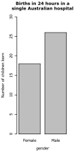 (a) A simple bar chart, giving number of data points in different categories
 -
 (b) Alternative, for highly ordered data: symbols mark number of data points, lines imply intermediate values are conceptually possible


Figure 2.1(a) displays these counts as a bar chart; another possibility is to use points as in Figure 2.1(b). In the case of gender, the order of the levels is not important: either 'male' or 'female' could come first. In the case of class, the natural order of the levels is used in the plot. In the extreme case, where intermediate levels might be meaningful, or where you wish to emphasise the pattern between levels, it may be reasonable to connect points by lines. For illustrative purposes, this has been done in Figure 2.1(b), although the reader may question whether it is appropriate in this instance.
plot(1:length(Gender), Gender, yaxs="n"); axis(2, 1:2, levels(Gender), las=1)
In some cases we may be interested in the actual sequence of data points. This is particularly so for time series data, but may also be relevant elsewhere. For instance, in the case of gender, the data was recorded in the order that each child was born. If we think that the preceeding birth influences the following birth (unlikely in this case, but just within the realm of possibility if pheremones are involved), then we might want to do Symbol-by-Symbol plot . If we are looking for associations with time, however, then a bivariate plot may be more appropriate ***, or there are particular features of the data that we are interested in (e.g. repeat rate), then other possibilities exist (doi:10.1016/j.stamet.2007.05.001).See chapter on time series
Quantitative variables
[edit | edit source]| landArea | |
| Alabama | 133666 |
|---|---|
| Alaska | 1527463 |
| Arizona | 295022 |
| Arkansas | 137538 |
| California | 411012 |
| Colorado | 269998 |
| Connecticut | 12973 |
| Delaware | 5327 |
| Florida | 151669 |
| Georgia | 152488 |
| Hawaii | 16705 |
| Idaho | 216411 |
| Illinois | 146075 |
| Indiana | 93993 |
| Iowa | 145790 |
| Kansas | 213062 |
| Kentucky | 104622 |
| Louisiana | 125673 |
| Maine | 86026 |
| Maryland | 27394 |
| Massachusetts | 21385 |
| Michigan | 150778 |
| Minnesota | 217735 |
| Mississippi | 123583 |
| Missouri | 180485 |
| Montana | 381085 |
| Nebraska | 200017 |
| Nevada | 286297 |
| New Hampshire | 24097 |
| New Jersey | 20295 |
| New Mexico | 315113 |
| New York | 128401 |
| North Carolina | 136197 |
| North Dakota | 183021 |
| Ohio | 106764 |
| Oklahoma | 181089 |
| Oregon | 251179 |
| Pennsylvania | 117411 |
| Rhode Island | 3144 |
| South Carolina | 80432 |
| South Dakota | 199550 |
| Tennessee | 109411 |
| Texas | 692404 |
| Utah | 219931 |
| Vermont | 24887 |
| Virginia | 105710 |
| Washington | 176616 |
| West Virginia | 62628 |
| Wisconsin | 145438 |
| Wyoming | 253596 |
| deathsPerYear | |
| 1875 | 3 |
|---|---|
| 1876 | 5 |
| 1877 | 7 |
| 1878 | 9 |
| 1879 | 10 |
| 1880 | 18 |
| 1881 | 6 |
| 1882 | 14 |
| 1883 | 11 |
| 1884 | 9 |
| 1885 | 5 |
| 1886 | 11 |
| 1887 | 15 |
| 1888 | 6 |
| 1889 | 11 |
| 1890 | 17 |
| 1891 | 12 |
| 1892 | 15 |
| 1893 | 8 |
| 1894 | 4 |
A quantitative variable can be plotted in many more ways than a categorical variable. Some of the most common single-variable plots are discussed below, using the land area of the 50 US states as our example of a continuous variable, and a famous data set of the number of deaths by horse kick as our example of a discrete variable. These data are tabulated in Tables 2.2 and 2.3
Some sorts of data consist of many data points with identical values. This is particularly true for count data where there are low numbers of counts (e.g. number of offspring).
There are 3 things we might want to look for in these sorts of plots
- points that seem extreme in some way (these are known as outliers). Outliers often reveal mistakes in data collection, and even if they don't, they can have a disproportionate effect on further analysis. If it turns out that they aren't due to an obvious mistake, one option is to remove them from the analysis, but this causes problems of its own/
- shape & position of the distribution (e.g. normal, bimodal, etc.)
- similarity to known distributions (QQ)
We'll keep the focus mostly on the variable "landArea" ***
 |
  |
  |
 |
The simplest way to represent quantitative data is to plot the points on a line, as in Figure 2.3(a). This is often called a 'dot plot, although this is also sometimes used to describe a number of other types of plot (e.g. Figure 2.7)[12]. To avoid confusion, it may be best to call it a one-dimensional scatterplot. As well as simplicity, there are two advantages to a 1D scatterplot
- All the information present in the data is retained.
- Outliers are easily identified. Indeed, it is often useful to be able to identify which data points are outliers. Some software packages allow you to identify points interactively (e.g. by clicking points on the plot). Otherwise, points can be labelled, as has been done for some outlying points in Figure 2.3a[13].
One dimensional scatterplots do not work so well for large datasets. Figure 2.3(a) consists of only 50 points. Even so, it is difficult to get an overall impression of the data, to (as the saying goes) "see the wood for the trees". This is partly because some points lie almost on top of each other, but also because of the sheer number of closely placed points. It is often the case that features of the data are best explored by summarising it in some way.
Figure 2.3(b) shows a step on the way to a better plot. To alleviate the problem of points obscuring each other, they have been displaced, or jittered sideways by a small, random amount. More importantly, the data have been summarised by dividing into quartiles (and coloured accordingly, for ease of explanation). The quarter of states with the largest area have been coloured red. The smallest quarter of states have been coloured green.
More generally, we can talk about the quantiles of our data[14]. The red line represents the 75% quantile: 75% of the points lie below it. The green line represents the 25% quantile: 25% of the points lie below it. The distance between these lines is known as the Interquartile Range (IQR), and is a measure of the spread of the data. The thick black line has a special name: the median. It marks the middle of the data, the 50% quantile: 50% of the points lie above, and 50% lie below. A major advantage of quantiles over other summary measures is that they are relatively insensitive to outliers, or changes in scale ****.
Figure 2.3(c) is a coloured version of a widely used statistical summary plot: the boxplot. Here it has been coloured to show the correspondence to Figure 2.3(b). The box marks the quartiles of the data, with the median marked within the box. If the median is not positioned centrally within the box, this is often an indicator that the data are skewed in some way. The lines on either side of the box are known as "whiskers", and summarise the data which lies outside of the upper and lower quartiles. In this case, the whiskers have simply been extended to the maximum and minimum observed values.
Figure 2.3(d) is a more sophisticated boxplot of the same data. Here, notches have been drawn on the box: these are useful for comparing the medians in different boxplots. The whiskers have been shortened so that they do not include points considered as outliers. There are various ways of defining these outliers automatically. This figure is based on a convention that considers outlying points as those more than one and a half times the IQR from either side of the box. However it is often more informative to identify and inspect interesting points (including outliers) by visual inspection. For example, in Figure 2.1a it is clear that Alaska and (to a lesser extent) Texas are unusually large states, but that California (identified as an outlier by this automatic procedure) is not so set-apart from the rest.
 |
 |
 |
 |
One problem with plotting on a single line is that, if points are repeated, there ***. This is particularly problematic for discrete data. NB, there is no particular reason (or established convention) for these plots to be vertical. Figure 2.2 shows . The stacked plot (Figure 2.4d) is similar to a histogram (Figure 2.5).
 |
  |
  |
  |
This gives another way of picturing the median & other quantiles: as dividing the area into sections ***
 |
 |
We can space out the points along the other axis. For example, if the order of points in the dataset is meaningful, we can just plot each point in turn. This is true for whatsit's horse-kick data. The data by year are plotted in Figure 2.6.
 |
  |
 |
One thing we can always do is to sort the data points by their value, plotting the smallest first, etc. This is seen in Figure 2.3b. If all the data points were equally spaced (and excluded each other****), we would see a straight line. The plot for the logged variables shows that this transformation has evened out the spacing somewhat. This is called a quantile plot, for the following reason
when the axes are swapped, this is called the empirical cumulative distribution function. The unswapped data is useful for understanding qq plots. Also for understanding quantiles. median, etc.
Transformations
[edit | edit source]We could put a scale break in, but a better option is usually to transform the variable.
  |
  |
 |
 |
Sometimes, plotting on a different scale (e.g. a logarithmic scale) can be more informative. We can visualise this either as a plot with a non-linear (e.g. logarithmic) axis, or as a conventional plot of a transformed variable (e.g. a plot of log(my.variable) on a standard, linear axis). Figure 2.1(b) illustrates this point: the left axis marks the state areas, the right axis marks the logarithm of the state areas. This sort of rescaling can highlight quite different features of a variable. In this case, it seems clear that there are a batch of nine states which seem distinctly smaller than most, and while Alaska still seems extraordinarily large, Texas does not seem so unusual in that respect. This is also reflected by the automatic labelling of outliers in the log-transformed variable.
It is particularly common for smaller numbers to have greater resolution. As discussed in later chapters ***, logarithmic scales are particularly useful for multiplicative data ***.
  |
  |
 |
 |
There are other common transformations, for example, the square-root transformation (often used for count data). This may be more appropriate for state areas, if the limiting factor for state size is (e.g.) the distance across the state, or factors associated with it (e.g. the length of time to cross from one side to another). Figure 2.1c shows a sqrt rescaling of the data. You can see that in some sense this is less extreme than the log transformation...
Univariate plots
stripchart(state.areas, xlab="Area (sq. miles)") #see method="stack" & method="jitter" for others
boxplot(sqrt(state.area))
hist(sqrt(state.area))
hist(sqrt(state.area), 25)
plot(density(sqrt(state.area))
plot(UKDriverDeaths)

qqnorm()
ecdf(
Datasets
[edit | edit source]Multiple variables in a table. Notation. most packages do this.
Bivariate plotting
[edit | edit source]Quantitative versus quantitative
[edit | edit source]Scatter plots problems with overplotting? Sunflowerplots etc.
Quantitative versus categorical
[edit | edit source]Vioplots (&boxplots)
Categorical versus categorical
[edit | edit source]Mosaicplots
Notes
[edit | edit source]- ↑ The convention (which is followed here) is to write variable names in italics
- ↑ These are special words in R, and cannot be used as names for objects. The objects
TandFare temporary shortcuts forTRUEandFALSE, but if you use them, watch out: since T and F are just normal object names you can change their meaning by overwriting them. - ↑ if the logical vector is shorter than the original vector, then it is sequentially repeated until it is of the right length
- ↑ Note that, when using continuous (fractional) numbers, rounding error may mean that results of calculations are not exactly equal to each other, even if they seem as if they should be. For this reason, you should be careful when using == with continuous numbers. R provides the function all.equal to help in this case
- ↑ But unlike
ifelse, it can't cope withNAvalues - ↑ For this reason, using
==inifstatements may not be a good idea, see the Note in?"=="for details. - ↑ These are particularly used in more advanced computer programming in R, see ?"&&" for details
- ↑ Similar examples are given in Chatfield ****
- ↑ There are actually 3 types of allowed numbers: "normal" numbers, complex numbers, and simple integers. This book deals almost exclusively with the first of these.
- ↑ This is not quite true, but unless you are a computer specialist, you are unlikely to use the final type: a vectors of elements storing "raw" computer bits, see
?raw - ↑ This dataset was collected by the Russian economist von Bortkiewicz, in 1898, to illustrate the pattern seen when events occur independently of each other (this is known as a Poisson distribution). The table here gives the total number of deaths summed over all 14 corps. For the full dataset, broken down into corp, see Statistical Analysis: an Introduction using R/Datasets
- ↑ Authors such as Wild & Seber call it a dot plot, but R uses the term "dotplot" to refer to a Cleveland (1985) dot-plot as shown in Figure 2.1(b). Other authors (***) specifically use it to refer to a sorted ("quantile") plot as used in Figure *** (cite)
- ↑ Labels often obscure the plot, so For plots intended only for viewing on a computer, it is possible to print labels in a size so small that they can only be seen when zooming in.
- ↑ There a many different methods for calculating the precise value of a quantile, when it lies between two points. See Hyndman and Fan (1996)
References
[edit | edit source]Carifio, J. & Perla, R. (2007). Ten Common Misunderstandings, Misconceptions, Persistent Myths and Urban Legends about Likert Scales and Likert Response Formats and their Antidotes. Journal of Social Sciences, 2, 106-116. http://www.scipub.org/fulltext/jss/jss33106-116.pdf