Fractals/Iterations in the complex plane/pcheckerboard
Task
[edit | edit source]How to show dynamics inside parabolic basin ?
Parameter c is a parabolic point
Attractor (limit set, attracting cycle / fixed point )
- belongs to Julia set ( not as in other cases )
- is weakly attracting ( lazy dynamics)
Algorithm
[edit | edit source]
Color depends on:
- sign of imaginary part of numerically approximated Fatou coordinate (numerical explanation )
- position of under in relation to one arm of critical orbit star: above or below ( geometric explanation)


- critical orbit is on the boundary between boxes and on the level curves of attraction time
-

-
_%3D_rho_*_z%5E2_*_(z-3)_over_(1-3z)_with_LCM_and_critical_orbit.png)
%3Dz%5E2_%2B_mz_where_p_over_q%3D1_over_3.svg)
Name of the algorithm
[edit | edit source]- Parabolic chessboard = parabolic checkerboard
- zeros of qn - use only interior of Filled Julia sets on real slice of Mandelbrot set ( c is a real number, iaginary part is zero)
- Binary decomposition ( method = BDM ) in parabolic case
- Tessellation of the Interior of Filled Julia Sets ( Tomoki Kawahira in Semiconjugacies in Complex Dynamics with Parabolics)
- internal tiling
Steps
[edit | edit source]First choose:
- choose target set, which is a circle with :
- center in parabolic fixed point
- radius such small that width of exterior between components is smaller then pixel width
- Target set consist of fragments of p components ( sectors). Divide each part of target set into 2 subsectors ( above and below critical orbit ) = binary decomposition
Steps:
- take = initial point of the orbit ( pixel)
- make forward iterations
- if points escapes = exterior
- if point do not escapes then check if point is near fixed point ( in the target set)
- if no then make some extra iterations
- if is then check in what half of target set it ( binary decomposition)

How to find trap ?
[edit | edit source]Steps for parabolic basin
- choose component with critical point inside
- choose trap
- decompose trap disk for binary decomposition = divide into 2 parts : above and beyond the critical orbit
Trap features:
- is inside component with critical point inside
- trap has parabolic point on it's boundary
- center of the trap is midpoint between last point of critical orbit and fixed point
- radius of the trap is half of distance between fixed point and last point of critical orbit

Target set
- for periods 1 and 2 in case of complex quadratic polynomial : circle
- for periods >2: curvilinear sectors of circle around fixed point, 2 triangles described by :
Nota that one trap for components is bigger then two traps for BDM
- trap for componets : triangle
- trap for BDM : triangle


where
- z1, z2 are the last point of external rays bounding component ( usually the biggest one, with critical point inside )
- is the critical point, or it's forward image in case thet critical orbit arm is not straight line
- is parabolic fixed point


Because of lazy dynamics one stops the computation before critical orbit and external rays land on the parabolic fixed point. The remaining gap is filled (approximated) with line from the last point to the landing point.
-
 computed and approximated parts

How to compute preimages of critical point ?
[edit | edit source]Here a and b are 2 inverse ( or backward ) iterations ( multivalued with argument adjusted ) used in the program Mandel by Wolf Jung:
- 1-st inverse function = key a =
- 2-nd inverse function = key b =


"Use the keys a and b for the inverse mapping. (The two branches are approximately mapping to the parts A and B of the itinerary.)
/* *****************************************************************************************
 *************************** inverse function of f(z) = z^2 + c ****************************
 *******************************************************************************************
*/

 /*f^{-1}(z) =  inverse with argument adjusted
    "When you write the real and imaginary parts in the formulas as complex numbers again,
       you see that it is sqrt( -c / |c|^2 )  *  sqrt( |c|^2 - conj(c)*z ) ,
     so this is just sqrt( z - c )  except for the overall sign:
    the standard square-root takes values in the right halfplane,  but this is rotated by the squareroot of -c .
    The new line between the two planes has half the argument of -c .
    (It is not orthogonal to c ...  )"
    ...
    "the argument adjusting in the inverse branch has nothing to do with computing external arguments.  It is related to itineraries and kneading sequences,  ...
    Kneading sequences are explained in demo 4 or 5, in my slides on the stripping algorithm, and in several papers by Bruin and Schleicher.

    W Jung " */
complex double fa(const complex double z0){

	double t = cabs(c);
  	t = t*t;
  	complex double z =  csqrt(-c/t)*csqrt(t-z0*conj(c));
  	return - z;


}

complex double fb(const complex double z0){

	double t = cabs(c);
  	t = t*t;
  	complex double z =  csqrt(-c/t)*csqrt(t-z0*conj(c));
  	return  z;


}


complex double give_preimage_a(complex double z0){

	int i;
	int iMax = child_period;
	complex double z = z0;


	for (i = 0; i < iMax; ++i){
		z = fa(z); }
	return z;

}


complex double give_preimage_b(complex double z0){

	int i;
	int iMax = child_period;
	complex double z = z0;


	for (i = 0; i < iMax-1; ++i){
		z = fa(z); }
	z = fb(z);
	return z;

}


int Draw_preimages(complex double z0, unsigned char iColor, unsigned char A[]){

	complex double z = z0;
	int i;
	int iMax = 100;


	for (i = 0; i < iMax; ++i){
		z = give_preimage_a(z);
 		dDrawPoint(z, iColor, A);
 		}

 	z = z0;

 	z = give_preimage_b(z);
 	dDrawPoint(z, iColor, A);
 	for (i = 0; i < iMax - 1; ++i){
		z = give_preimage_a(z);
 		dDrawPoint(z, iColor, A);
 		}


	return 0;
}
dictionary
[edit | edit source]- The chessboard is the name of this decomposition of A into a graph and boxes
- the chessboard graph
- the chessboard boxes :" The connected components of its complement in A are called the chessboard boxes (in an actual chessboard they are called squares but here they have infinitely many corners and not just four). " [1]
- the two principal or main chessboard boxes
- trap = target set = attracting petal
Visualizing Structures with the Chessboard Graph
"An often used and very useful technique of visualization of ramified covers (and partial cover structures that are not too messy) consists in cutting the range in domains, often simply connected, along lines joining singular values, and taking the pre-image of these pieces, which gives a new set of pieces. The way they connect together and the way they map to the range give information about the structure." Arnaud Chéritat Near Parabolic Renormalization for Unicritical Holomorphic Maps by Arnaud Chéritat
_%3D_z%5E2_%2B0.25.svg)
description
[edit | edit source]"A nice way to visualize the extended Fatou coordinates is to make use of the parabolic graph and chessboard." [2]
Color points according to :[3]
- the integer part of Fatou coordinate
- the sign of imaginary part
Corners of the chessboard ( where four tiles meet ) are precritical points [4]

or

1/1
[edit | edit source]The parabolic chessboard for the polynomial z + z^2 normalizing * each yellow tile biholomorphically maps to the upper half plane * each blue tile biholomorphically maps to the lower half plane under * The pre-critical points of or equivalently the critical points of are located where four tiles meet"[5]


Images
[edit | edit source]Click on the images to see the code and descriptions on the Commons !
- basins
-
 BDM only in the interior
 -
 BDM in both exterior ( superattracting) and interior ( parabolic)
 -
 only one basin: exterior ( superattracting)
_%3D_z*z_%2B_0.25.png)


- on the real slice of Mandelbrot set
-
 on the cusp of main cardioid
 -

-
 from main cardioid to period 2
 -
 between period 2 and 4 along 1/2 ray


- on the boundary of main cardioid of Mandelbrot set
-
0/1 = 1/1
-
1/2
-
 1/3
1/3 -
 1/4
1/4 -
 5/11
5/11

_%3D_z*z_%2B_0.25%2B0.5i_BDM.png)
_%3D_z*z_-0.6900598700150440%2B0.2760264827846140i_BDM.png)
evolution on the escape route 0
- start with nucleus of component with period 1 (c = 0)
- go along internal ray for angle = 0
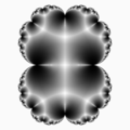
- parabolic point (c = 1/4)
- on the external ray for angle 0
- evolution on the internal ray of the main cardioid of Mandelbrot set
-
-
 superattracting
 -
 attracting
 -
parabolic
-
only one basin: exterior ( superattracting), Julia set discontinous


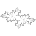
- other polynomials
-
 various number of star branches
_%3D_z%5E4_-_z_with_various_number_of_star_branches.gif)
- orbits inside sepals
-
0/1 = 1/1
-
 invariant curves inside main boxes
 -
-


- only boundaries of parabolic BDM
-
 d=2
d=2 -
 d=3
d=3 -
 d=4
d=4 -
 d=5
d=5 -
-

-

-
_%3D_(z%5Ed_%2B_a)_over_(1_%2B_a*z%5Ed)_with_a_%3D_(d_-_1)_over_(_d_%2B_1)_for_d_%3D_2.png)
_%3D_(z%5Ed_%2B_a)_over_(1_%2B_a*z%5Ed)_with_a_%3D_(d_-_1)_over_(_d_%2B_1)_for_d_%3D_3.png)
_%3D_(z%5Ed_%2B_a)_over_(1_%2B_a*z%5Ed)_with_a_%3D_(d_-_1)_over_(_d_%2B_1)_for_d_%3D_4.png)
_%3D_(z%5Ed_%2B_a)_over_(1_%2B_a*z%5Ed)_with_a_%3D_(d_-_1)_over_(_d_%2B_1)_for_d_%3D_5.png)
_%3D_z%5E3_%2B_0.3849001794597505.png)
_%3D_z*z*z*z_%2B_0.472464424146544.png)
_%3D_z*z*z*z*z_%2B_0.5349922439811376.png)
-
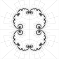
 structural chessboard of first renormalization of the degree 2 parabolic Blaschke product, cylinders highted with a normal map.

Examples :
- Tiles: Tessellation of the Interior of Filled Julia Sets by T Kawahira[6]
- coloured cauliflower by A Cheritat [7]
code
[edit | edit source]For the internal angle 0/1 and 1/2 critical orbit is on the real line ( Im(z) = 0). It is easy to compute parabolic chessboard because one have to check only imaginary part of z. For other cases it is not so easy
0/1
[edit | edit source]Cpp code by Wolf Jung see function parabolic from file mndlbrot.cpp ( program mandel ) [8][9]
To see effect :
- run Mandel
- (on parameter plane ) find parabolic point for angle 0, which is c=0.25. To do it use key c, in window input 0 and return.
C code :
  // in function uint mndlbrot::esctime(double x, double y)
  if (b == 0.0 && !drawmode && sign < 0
      && (a == 0.25 || a == -0.75)) return parabolic(x, y);
 // uint mndlbrot::parabolic(double x, double y)
 if (Zx>=0 && Zx <= 0.5 && (Zy > 0 ? Zy : -Zy)<= 0.5 - Zx)
            { if (Zy>0) data[i]=200; // show petal
                     else data[i]=150;}
Gnuplot code :
reset
f(x,y)=  x>=0 && x<=0.5 &&  (y > 0 ? y : -y) <= 0.5 - x
unset colorbox
set isosample 300, 300
set xlabel 'x'
set ylabel 'y'
set sample 300
set pm3d map
splot [-2:2] [-2:2] f(x,y)
1/2 or fat basilica
[edit | edit source]Cpp code by Wolf Jung see function parabolic from file mndlbrot.cpp ( program mandel ) [10] To see effect :
- run Mandel
- (on parameter plane ) find parabolic point for angle 1/2, which is c=-0.75. To do it use key c, in window input 0 and return.
C code :
  // in function uint mndlbrot::esctime(double x, double y)
  if (b == 0.0 && !drawmode && sign < 0
      && (a == 0.25 || a == -0.75)) return parabolic(x, y);
 // uint mndlbrot::parabolic(double x, double y)
  if (A < 0 && x >= -0.5 && x <= 0 && (y > 0 ? y : -y) <= 0.3 + 0.6*x)
      {  if (j & 1) return (y > 0 ? 65282u : 65290u);
         else return (y > 0 ? 65281u : 65289u);
      }
-
 trap for components
 -

-
-

_Julia_set.png)

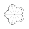
1/3
[edit | edit source]-
chessboard
-
 target set ( precritical points)

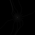
Numerical approximation of Julia set for fc(z)= z^2 + c
child_period  = 3
internal argument in turns = 1 / 3
parameter c = -0.1250000000000000 +0.6495190528383290*I
fixed point alfa z = a = -0.2500000000000000 +0.4330127018922194*I
external angles of rays landing on the fixed point  : t = 1/7 	t = 2/7 	t = 4/7
critical point z = zcr = 0.0000000000000000 +0.0000000000000000*I
precritical point z = z_precritical = -0.2299551351162811 -0.1413579816050052*I
external argument in turns of first ray landing on fixed point = 1 / 7
1/4
[edit | edit source]-
BDM for both exterior and interior
Julia set for fc(z)= z^2 + c
internal argument in turns = 1/4
parameter c = 0.2500000000000000 +0.5000000000000000*I
fixed point alfa z = a = 0.0000000000000000 +0.5000000000000000*I
critical point z = zcr = 0.0000000000000000 +0.0000000000000000*I
precritical point z = z_precritical = -0.2288905993372869 -0.0151096456992677*I
external angles of rays landing on fixed point: 1/15, 2/15, 4/15, 8/15 ( in turns)
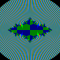
5/11
[edit | edit source]-
-
-
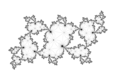
extarnal rays and critical orbit (11-arm star)
_%3D_z*z_-0.6900598700150440%2B0.2760264827846140i.png)
Numerical approximation of Julia set for fc(z)= z^2 + c
parameter c = ( -0.6900598700150440 ; 0.2760264827846140 )
fixed point alfa z = a = ( -0.4797464868072486 ; 0.1408662784207147 )
external angle of ray landing on fixed point: 341/2047
See also
[edit | edit source]- parabolic perturbation
- Checkerboard in Hyperbolic tilings by User:Tamfang : images and Python code
- https://plus.google.com/110803890168343196795/posts/Eun6pZVkkmA
- shadertoy: Orbit trapped julia Created by maeln in 2016-Jan-19
- Holomorphic checkerboard by etale_cohomology
- Sepals of cauliflower
- wikipedia :Zebra striping in computer graphics
- aproximation cauliflower by the true tree: tree which converge to the cauliflower julia set. the set of vertices is in one to one correspondence with the grand orbit of the critical point of z squared plus one quarter.[11]
references
[edit | edit source]- ↑ Near parabolic renormalization for unisingular holomorphic maps by Arnaud Cheritat
- ↑ About Inou and Shishikura’s near parabolic renormalization by Arnaud Cheritat
- ↑ Applications of near-parabolic renormalization by Mitsuhiro Shishikura
- ↑ Complex Dynamical Systems by Robert L. Devaney, page
- ↑ Antiholomorphic Dynamics: Topology of Parameter Spaces and Discontinuity of Straightening by Sabyasachi Mukherjee
- ↑ tiles by T Kawahira
- ↑ checkerboards by A Cheritat
- ↑ commons:Category:Fractals created with Mandel
- ↑ Program Mandel by Wolf Jung
- ↑ Program Mandel by Wolf Jung
- ↑ Oleg Ivrii (Tel Aviv University), "Shapes of trees"