Algorithms/Mathematical Background
Top, Chapters: 1, 2, 3, 4, 5, 6, 7, 8, 9, A
Before we begin learning algorithmic techniques, we take a detour to give ourselves some necessary mathematical tools. First, we cover mathematical definitions of terms that are used later on in the book. By expanding your mathematical vocabulary you can be more precise and you can state or formulate problems more simply. Following that, we cover techniques for analysing the running time of an algorithm. After each major algorithm covered in this book we give an analysis of its running time as well as a proof of its correctness
Asymptotic Notation
[edit | edit source]In addition to correctness another important characteristic of a useful algorithm is its time and memory consumption. Time and memory are both valuable resources and there are important differences (even when both are abundant) in how we can use them.
How can you measure resource consumption? One way is to create a function that describes the usage in terms of some characteristic of the input. One commonly used characteristic of an input dataset is its size. For example, suppose an algorithm takes an input as an array of integers. We can describe the time this algorithm takes as a function written in terms of . For example, we might write:
where the value of is some unit of time (in this discussion the main focus will be on time, but we could do the same for memory consumption). Rarely are the units of time actually in seconds, because that would depend on the machine itself, the system it's running, and its load. Instead, the units of time typically used are in terms of the number of some fundamental operation performed. For example, some fundamental operations we might care about are: the number of additions or multiplications needed; the number of element comparisons; the number of memory-location swaps performed; or the raw number of machine instructions executed. In general we might just refer to these fundamental operations performed as steps taken.
Is this a good approach to determine an algorithm's resource consumption? Yes and no. When two different algorithms are similar in time consumption a precise function might help to determine which algorithm is faster under given conditions. But in many cases it is either difficult or impossible to calculate an analytical description of the exact number of operations needed, especially when the algorithm performs operations conditionally on the values of its input. Instead, what really is important is not the precise time required to complete the function, but rather the degree that resource consumption changes depending on its inputs. Concretely, consider these two functions, representing the computation time required for each size of input dataset:
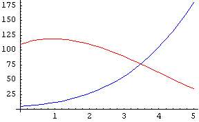
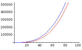
They look quite different, but how do they behave? Let's look at a few plots of the function ( is in red, in blue):
 |
 |
 |
 |
In the first, very-limited plot the curves appear somewhat different. In the second plot they start going in sort of the same way, in the third there is only a very small difference, and at last they are virtually identical. In fact, they approach , the dominant term. As n gets larger, the other terms become much less significant in comparison to n3.
As you can see, modifying a polynomial-time algorithm's low-order coefficients doesn't help much. What really matters is the highest-order coefficient. This is why we've adopted a notation for this kind of analysis. We say that:
We ignore the low-order terms. We can say that:
This gives us a way to more easily compare algorithms with each other. Running an insertion sort on elements takes steps on the order of . Merge sort sorts in steps. Therefore, once the input dataset is large enough, merge sort is faster than insertion sort.
In general, we write
when
That is, holds if and only if there exists some constants and such that for all is positive and less than or equal to .
Note that the equal sign used in this notation describes a relationship between and instead of reflecting a true equality. In light of this, some define Big-O in terms of a set, stating that:
when
Big-O notation is only an upper bound; these two are both true:
If we use the equal sign as an equality we can get very strange results, such as:
which is obviously nonsense. This is why the set-definition is handy. You can avoid these things by thinking of the equal sign as a one-way equality, i.e.:
does not imply
Always keep the O on the right hand side.
Big Omega
[edit | edit source]Sometimes, we want more than an upper bound on the behavior of a certain function. Big Omega provides a lower bound. In general, we say that
when
i.e. if and only if there exist constants c and n0 such that for all n>n0 f(n) is positive and greater than or equal to cg(n).
So, for example, we can say that
- , (c=1/2, n0=4) or
- , (c=1, n0=3),
but it is false to claim that
Big Theta
[edit | edit source]When a given function is both O(g(n)) and Ω(g(n)), we say it is Θ(g(n)), and we have a tight bound on the function. A function f(n) is Θ(g(n)) when
but most of the time, when we're trying to prove that a given , instead of using this definition, we just show that it is both O(g(n)) and Ω(g(n)).
Little-O and Omega
[edit | edit source]When the asymptotic bound is not tight, we can express this by saying that or The definitions are:
- f(n) is o(g(n)) iff and
- f(n) is ω(g(n)) iff
Note that a function f is in o(g(n)) when for any coefficient of g, g eventually gets larger than f, while for O(g(n)), there only has to exist a single coefficient for which g eventually gets at least as big as f.
Big-O with multiple variables
[edit | edit source]Given a functions with two parameters and ,
if and only if .
For example, , and .
Algorithm Analysis: Solving Recurrence Equations
[edit | edit source]Merge sort of n elements: This describes one iteration of the merge sort: the problem space is reduced to two halves (), and then merged back together at the end of all the recursive calls (). This notation system is the bread and butter of algorithm analysis, so get used to it.
There are some theorems you can use to estimate the big Oh time for a function if its recurrence equation fits a certain pattern.
Substitution method
[edit | edit source]Formulate a guess about the big Oh time of your equation. Then use proof by induction to prove the guess is correct.
Summations
[edit | edit source]
Draw the Tree and Table
[edit | edit source]This is really just a way of getting an intelligent guess. You still have to go back to the substitution method in order to prove the big Oh time.
The Master Theorem
[edit | edit source]Consider a recurrence equation that fits the following formula:
for a ≥ 1, b > 1 and k ≥ 0. Here, a is the number of recursive calls made per call to the function, n is the input size, b is how much smaller the input gets, and k is the polynomial order of an operation that occurs each time the function is called (except for the base cases). For example, in the merge sort algorithm covered later, we have
because two subproblems are called for each non-base case iteration, and the size of the array is divided in half each time. The at the end is the "conquer" part of this divide and conquer algorithm: it takes linear time to merge the results from the two recursive calls into the final result.
Thinking of the recursive calls of T as forming a tree, there are three possible cases to determine where most of the algorithm is spending its time ("most" in this sense is concerned with its asymptotic behaviour):
- the tree can be top heavy, and most time is spent during the initial calls near the root;
- the tree can have a steady state, where time is spread evenly; or
- the tree can be bottom heavy, and most time is spent in the calls near the leaves
Depending upon which of these three states the tree is in T will have different complexities:
Given for a ≥ 1, b > 1 and k ≥ 0:
- If , then (top heavy)
- If , then (steady state)
- If , then (bottom heavy)
For the merge sort example above, where
we have
thus, and so this is also in the "steady state": By the master theorem, the complexity of merge sort is thus
- .
Amortized Analysis
[edit | edit source][Start with an adjacency list representation of a graph and show two nested for loops: one for each node n, and nested inside that one loop for each edge e. If there are n nodes and m edges, this could lead you to say the loop takes O(nm) time. However, only once could the innerloop take that long, and a tighter bound is O(n+m).]


