Routing protocols and architectures/Print version
| This is the print version of Routing protocols and architectures You won't see this message or any elements not part of the book's content when you print or preview this page. |
The current, editable version of this book is available in Wikibooks, the open-content textbooks collection, at
https://en.wikibooks.org/wiki/Routing_protocols_and_architectures
Forwarding and routing
Routing is the process which determines the 'best' path for a packet and sends it out toward the destination:
- routing algorithm: it is in charge of deciding the paths to take for incoming packets:
- it determines the destinations reachable by each node;
- it computes the best paths (according to certain criteria) in a cooperative way with the other nodes;
- it stores local information in each node;
- forwarding algorithm: it is in charge of taking the path decided for each incoming packet:
- it performs a lookup in the local information computed and stored by the routing algorithm;
- it sends the outgoing packet along the best path.
Routing protocols differentiate into two classes:
- Interior Gateway Protocol (IGP): it includes the protocols used in intra-domain routing (e.g. RIP, IGRP, OSPF) to propagate routing information inside an Autonomous System[1];
- Exterior Gateway Protocol (EGP): it includes the protocols used in inter-domain routing (e.g. BGP) to propagate routing information between Autonomous Systems.
According to the OSI model, routing is a feature proper to the network layer, but it can be implemented at different layers:
- routing is implemented altogether at the network layer by protocols such as IP, X.25 and OSI/Decnet;
- some of the routing algorithms are implemented at the data-link layer by protocols such as Frame Relay and ATM and by bridges in switched LANs.
Modern routers implement two tables:
- Routing Information Base (RIB): it is the classical routing table listing all the destinations reachable within the network;
- Forwarding Information Base (FIB): it is a routing table optimized to speed up packet forwarding:
- dedicated hardware: TCAMs are able to store bits whose possible values are 0, 1 and 'don't care' → the netmask is integrated in the network address itself: each bit in the aggregated part has value 'don't care';
- cache: the FIB only includes the last used destination addresses;
- additional information: output port, destination MAC address.
Forwarding algorithms[edit | edit source]
Routing by network address[edit | edit source]
- Each node is identified by a network address.
- Each packet contains the address of the destination node.
- Each node contains the list of the reachable destination addresses with their corresponding next hops.
When a packet comes, the node uses the destination address included in it as the 'key' in the forwarding table to find the next hop.
- Advantage
It is a simple and efficient algorithm because it is stateless: packet forwarding takes place regardless of the forwarding of other packets, that is the node once a packet is forwarded will forget about it.
- Disadvantage
It is not possible to select different routes for the same destination based on the kind of traffic for quality of service.
- Adoption
Connectionless protocols (such as IP) typically use this forwarding algorithm.
'Coloured path' technique[edit | edit source]
- Each path between two nodes is identified by a PathID ('color').
- Each path contains a label corresponding to the PathID of the path to follow.
- Each node contains the lists of PathIDs with their corresponding output ports.
When a packet comes, the node uses the label included in it as the 'key' in the forwarding table to find the output port.
- Advantage
Several paths towards the same destination are possible → it is possible to choose the best path based on the kind of traffic for quality of service.
- Disadvantage
The PathID is global:
- path 'colouring' must be coherent on all the nodes over the network;
- scalability: the number of possible paths between all the node pairs in the network is very big → a lot of bits are needed to encode each PathID, and it is hard to find an identifier which has not been used yet.
Label swapping[edit | edit source]

The forwarding table in each node contains the mapping between the labels of the input ports and the labels of the output ports, including entries like:
When a packet comes, the node uses the label included in it and the input port as the 'key' in the forwarding table to find the output port, and it replaces the current label in the packet with the output label.
- Advantages
- scalability: the PathID of the path to follow is not global, but the label is decided locally node by node, and it must be coherent only between the nodes to the link endpoints:
- labels are made up of less bits because they have to encode less paths;
- each node must know only the labels of the paths crossing it → the forwarding table is smaller;
- efficiency: label swapping is fast with respect to forwarding algorithms such as 'longest prefix matching' in IP.
- Adoption
Label swapping is used by:
- telecommunication-derived network technologies (e.g. X.25, Frame Relay, ATM): label swapping allows quality of service, a feature considered as important by the world of phone operators;
- MPLS: in the backbone paths are in a fairly limited number and quite stable because they are created not end-to-end but in the MPLS cloud, where the network topology changes less frequently and traffic is more regular with respect to edges.
Path setup[edit | edit source]
When a host wants to generate and send the first packet toward a destination, how does it ask for setup of a new path and which label should it use?
- Manual setup
Paths and their corresponding labels are manually set by the network administrator.
Disadvantages
- high risk of human configuration mistakes;
- no automatic re-routing in case of faults;
- not suitable for highly dynamic networks where users frequently ask for new paths.
- On-demand setup
A signaling phase for path setup, that is for preparing labels in every node, is required, after which the host learns the label to use and it can send the first packet toward the destination.
Advantages
Quality of service is simpler:
- it is possible to set up different paths based on the source asking for its setup (e.g. the rector can have a path privileged compared to the researcher);
- it is possible to include inside the signaling packet a piece of information specifying how much bandwidth to reserve for the path.
Disadvantages
- complexity: signaling is achieved through another forwarding technique (e.g. routing by network address) over a dedicated circuit → complexity increases because the network must now manage two different forwarding techniques;
- scalability: if the path is long and the number of nodes to cross is high, the signaling phase may last too long, especially if the communication sessions are quite short like in the network world.
Source routing[edit | edit source]
The sender host writes into the packet itself the whole path which must follow to arrive at the destination.
- Advantage
Internal routers in the network are extremely simple.
- Disadvantage
The sender host must know the network topology and must interact directly with the other hosts in order to be able to compute paths → this breaks the paradigm according to which end users should just send packets and the network is in charge of forwarding packets toward their destinations.
- Adoption
IPv4 and IPv6 contemplate an option affecting the path of packets.
Comparison[edit | edit source]
- Routing by network address
- + simplicity: no setup, no state
- + scalability (forwarding): no 'per-session' state (stateless)
- − efficiency: big packet header
- − scalability (routing): very big routing table
- − reliability: difficult to guarantee the service
- − multipath: it does not support multiple paths between two entities
- Label swapping
- + scalability (routing): reduced routing table
- + efficiency: small packet header
- + guarantee of service: possibility to guarantee the service (path booking)
- + multipath: multiple paths allowed between two entities
- − scalability (setup): processing of the packets for path setup (critical with 'short' sessions)
- − scalability (forwarding): 'per-session' state (needed for quality of service)
- − complexity: path setup (path setup process, ad-hoc forwarding for path setup packets)
- Source routing
- + efficiency (routers): intermediate systems are extremely simple
- − efficiency (sources): end systems should worry about computing paths
References[edit | edit source]
- ↑ An Autonomous System (AS) is generally the network under the control of an ISP.
Routing algorithms
| Routing algorithms presented in the following assume they work on a network based on routing by network address. |
A routing algorithm is a process of collaborative type in charge of deciding, in every intermediate node, the directions which must be used to reach destinations:
- it determines the destinations reachable by each node:
- it generates information about the reachability of local networks: the router informs its neighbor routers that the local network exists and it is reachable through it;
- it receives information about the reachability of remote networks: a neighbor router informs the router that the remote network exists and it is reachable through it;
- it propagates information about the reachability of remote networks: the router informs the other neighbor routers that the remote network exists and it is reachable through it;
- it computes optimal paths (next hops), in a cooperative way with the other nodes, according to certain criteria:
- a metric has to be established: a path may be the best one based on a metric but not based on another metric;
- criteria must be coherent among all the nodes in the network to avoid loops, black holes, etc.;
- the algorithm must operate automatically to avoid human errors in manual configuration and to favor scalability;
- it stores local information in the routing table of each node: a routing algorithm is not required to know the entire topology of the network, but it is only interested in building the correct routing table.
- Characteristics of an ideal routing algorithm
- simple to implement: less bugs, easy to understand, etc.;
- lightweight to execute: routers should spend as less resources as possible in running the algorithm because they have limited CPU and memory;
- optimal: the computed paths should be optimal according to the chosen metrics;
- stable: it should switch to another path just when there is a topology or a cost change to avoid route flapping, that is the frequent change of preferred routes with consequent excess of transient periods;
- fair: it should not favour any particular node or path;
- robust: it should be able to automatically adapt to topology or cost changes:
- fault detection: it should not rely on external components to detect a fault (e.g. a fault can not be detected at the physical layer if it occurs beyond a hub);
- auto-stabilization: in case of variations in the network it should converge to a solution without any external intervention (e.g. explicit manual configuration);
- byzantine robustness: it should recognize and isolate a neighbor node which is sending fake information, due to a fault or a malicious attack.
Internet does not implement byzantine robustness, but it is based on confidence → faults and malicious behaviours require human intervention.
- Classification of routing algorithms
- non-adaptive algorithms (static): they take decisions independently of how the network is:
- static routing (or fixed directory routing)
- random walk
- flooding, selective flooding
- adaptive algorithms (dynamic): they learn information about the network to better take decisions:
- centralized routing
- isolated routing: hot potato, backward learning
- distributed routing: Distance Vector, Link State
- hierarchical algorithms: they allow routing algorithms to scale up on wide infrastructures.
Metric[edit | edit source]
A metric is the measure of how good a path is, obtained by transforming a physical quantity (e.g. distance, transmission speed), or a combination of them, in numerical form (cost), in order to choose the least-cost path as the best path.
A best metric does not exist for all the kinds of traffic: for example bandwidth is suitable for file-transfer traffic, while transmission delay is suitable for real-time traffic. The choice of the metric can be determined from the 'Type of Service' (TOS) field in the IP packet.
- Issues
- (non-)optimization: the primary task of routers is to forward users' traffic, not to spend time in computing paths → it is better to prefer solutions which, even if they are not fully optimized, do not compromise the primary functionality of the network and do not manifest problems which can be perceived by the end user:
- complexity: the more criteria are combined, the more complex the algorithm becomes and the more computational resources at run-time it requires;
- stability: a metric based on the available bandwidth on the link is too unstable, because it depends on the instantaneous traffic load which is very variable in time, and may lead to route flapping;
- inconsistency: metrics adopted by nodes in the network must be coherent (for every packet) to avoid the risk of loops, that is packet 'bouncing' between two routers using different conflicting metrics.
Transients[edit | edit source]
Modern routing algorithms are always 'active': they exchange service messages all the time to detect faults autonomously. However, they do not change the routing table unless a status change is detected:
- topology changes: link fault, addition of a new destination;
- cost changes: for example a 100-Mbps link goes up to 1 Gbps.
Status changes result in transient phases: all the nodes in a distributed system can not be updated at the same time, because a variation is propagated throughout the network at a finite speed → during the transient, status information in the network may not be coherent: some nodes already have new information (e.g. the router detecting the fault), while other ones still have old information.
Not all status changes have the same impact on data traffic:
- positive status changes: the effect of the transient is limited because the network may just work temporarily in a sub-optimal condition:
- a path gets a better cost: some packets may keep following the old path now become less convenient;
- a new destination is added: the destination may appear unreachable due to black holes along the path towards it;
- negative status changes: the effect of the transient manifests itself more severely to the user because it interferes also with the traffic that should not be affected by the fault:
- a link fault occurs: not all routers have learnt that the old path is no longer available → the packet may start `bouncing' back and forth saturating the alternative link (routing loop);
- a path worsens its cost: not all routers have learnt that the old path is no longer convenient → analogous to the case of fault (routing loop).
In general, two common problems affect routing algorithms during the transient: black holes and routing loops.
Black holes[edit | edit source]
A black hole is defined as a router which, even if at least a path exists through which it could reach a certain destination, does not know any of them (yet).
- Effect
The effect on data traffic is limited to packets directed toward the concerned destination, which are dropped until the node updates its routing table and acquires information about how to reach it. Traffic directed to other destinations is not affected by the black hole at all.
Routing loops[edit | edit source]
A routing loop is defined as a cyclic path from the routing point of view: a router sends a packet on a link but, because of an inconsistency in routing tables, the router at the other endpoint of the link sends it back.
- Effect
Packets directed toward the concerned destination start 'bouncing' back and forth (bouncing effect) → the link gets saturated → also traffic directed to other destinations crossing that link is affected.
Backup route[edit | edit source]
Backup route is a concept mostly used in telephone networks based on a hierarchical organization: every exchange is connected to an upper-level exchange by a primary route, and to another upper-level exchange by a backup route → if a fault occurs in the primary route, the backup route is ready to come into operation without any transient period.
A data network is instead based on a meshed topology, where routers are interconnected in various ways → it is impossible to foresee all possible failures of the network to prearrange backup paths, but when a failure occurs a routing algorithm is preferable automatically computing on the fly an alternative path (even if the computational step requires a transient period).
Backup route in modern networks can still have applications:
- a company connected to the Internet via ADSL can keep its connectivity when the ADSL line drops by switching to a backup route via HiperLAN technology (wireless);
- the internet backbone is by now in the hands of telephone companies, which have modeled it according to criteria of telephone networks → its organization is hierarchical enough to allow backup routes to be prearranged.
Multipath routing[edit | edit source]
With routing by network address, all the packets toward a destination follow the same path, even if alternative paths are available → it would be preferable to make part of traffic follow an alternative path, even if more costly, not to saturate the path chosen by the algorithm.
Multipath routing, also known as 'load sharing', is a traffic engineering feature aiming at distributing traffic toward the same destination over multiple paths (when available), allowing multiple entries for each destination in the routing table, for a more efficient usage of network resources.
Unequal-cost multipath routing[edit | edit source]
An alternative path is used only if it has cost not too greater than cost of the least-cost primary path:


Traffic is distributed inversely proportionally to the cost of the routes. For example in this case:

the router may decide to send the packet with 66\% probability along the primary path and 33\% probability along the secondary path.
- Problem
Given a packet, each router autonomously decides on which path to forward it → incoherent decisions between routers may make the packet enter a routing loop, and since the forwarding is usually session-based that packet will never exit the loop:

Equal-cost multipath routing[edit | edit source]
An alternative path is used only if it has cost exactly equal to cost of the primary path ():


Traffic is equally partitioned on both the paths (50%).
- Problems
If the first packet follows the slow path and the second packet follows the fast path, TCP mechanisms may cause overall performance to get worse:
- Problems caused by equal-cost multipath routing.
-
 TCP reordering problem.
 -
 Transmission rate decrease.


- TCP reordering problem: packets may arrive out of sequence: the second packet arrives at the destination before the first packet → the process for sequence number reordering keeps busy the computational resources of the receiver;
- transmission rate decrease: if the acknowledgment packet (ACK) of the first packet arrives too late, the source thinks that the first packet went lost → when 3 duplicate (cumulative) ACKs have arrived and the timeout expires, TCP sliding-window mechanisms get into the action:
- fast retransmit: the source unnecessarily transmits again the packet → the packet gets duplicate;
- fast recovery: the source thinks that the network is congested → it slows down packet sending by limiting the transmission window: it sets the threshold value to half of the current value of the congestion window, and makes the congestion window restart from value 1 (that is only one packet at a time is sent and its ACK is awaited before sending the next packet).
Criteria[edit | edit source]
Real multipath routing implementations split traffic so that traffic toward a same destination follows the same path:
- flow-based: every transport-layer session is identified by the quintuple:
- <source IP address>
- <destination IP address>
- <transport-layer protocol type> (e.g. TCP)
- <source port>
- <destination port>
and the router stores a table mapping session identifiers with output ports:
- extracting the fields forming the session ID from the packet is onerous, due to the variety of supported packet formats (VLAN, MPLS...);
- information about transport-layer ports is unavailable in case of fragmented IP packets;
- searching the session ID table for the quintuple is onerous;
- often TCP connection shutdown is not 'graceful leaving', that is FIN and ACK packets are not sent → entries in the session ID tables are not cleared → it is required a thread performing sometimes a cleanup of old entries by looking at their timestamps;
- packet-based: the router sends the packets having even (either destination or source or both) IP address to a path, and odd IP address to the other path → the hashing operation is very fast.
- Problem
Traffic toward a same destination can not use both the paths at the same time → there are troubles in case of very big traffic toward a certain destination (e.g. a nightly backup between two servers).
Non-adaptive algorithms[edit | edit source]
Static routing[edit | edit source]
The network administrator manually configures on each router its routing table.
- Disadvantage
If a change in the network occurs, routing tables need to be manually updated.
- Application
Static routing is mainly used on routers at the network edges:

- edge routers are not allowed to propagate routing information toward the backbone: the core router stops all the advertisements coming from the edge, otherwise a user could advertise a network with the same address as an existing network (e.g. google.com) and redirect towards him a part of traffic directed to that network.
Since users can not advertise their own networks, how can they be reachable from outside? The ISP, which knows which addresses are used by the networks it sold to users, must configure the core router so that it advertises those networks to other routers even if they are not locally connected; - edge routers are not allowed to receive routing information from the backbone: an edge router is typically connected by a single link to a core router → a global default route is enough to reach the entire Internet.
Random walk[edit | edit source]
When a packet arrives, the router chooses a port randomly (but the one from which it was received) and sends it out on that port.
- Applications
It is useful when the probability that the packet reaches the destination is high:
- peer-to-peer (P2P) networks: for contents lookup;
- sensor network: sending messages should be a low-power operation.
Flooding[edit | edit source]
When a packet arrives, the router sends it out on all the ports (but the one from which it was received).
Packets may have a 'hop count' field to limit flooding to a network portion.
- Applications
- military applications: in case of attack the network could be damaged → it is critical that the packet arrives at destination, even at the cost of having a huge amount of duplicate traffic;
- Link State algorithm: each router when receiving the network map by a neighbor has to propagate it to the other neighbors:
 A4. The Link State algorithm#Flooding algorithm.
Selective flooding[edit | edit source]
When a packet arrives, the router first checks if it has already received and flooded it in the past:
- old packet: it discards it;
- new packet: it stores and sends it out on all the ports (but the one from which it was received).
Each packet is recognized through the sender identifier (e.g. the source IP address) and the sequence number:
- if the sender disconnects from the network or shutdowns, when it connects again the sequence number will restart from the beginning → the router sees all the received packets as old packets;
- sequence numbers are encoded on a limited number of bits → the sequence number space should be chosen so as to minimize new packets wrongly recognized as old packets.
Sequence number spaces[edit | edit source]
- Linear space
It can be tolerable if selective flooding is used for few control messages:
- when the sequence number reaches the maximum possible value, an overflow error occurs;
- old packet: the sequence number is lower than the current one;
- new packet: the sequence number is greater than the current one.
- Circular space
It solves the sequence number space exhaustion problem, but it fails if a packet arrives with sequence number too far away from the current one:
- when the sequence number reaches the maximum possible value, the sequence number restarts from the minimum value;
- old packet: the sequence number is in the half preceding the current one;
- old packet: the sequence number is in the half following the current one.
- Lollipop space
The first half of the space is linear, the second half is circular.
Adaptive algorithms[edit | edit source]
Centralized routing[edit | edit source]
All routers are connected to a centralized control core called Routing Control Center (RCC): every router tells the RCC which its neighbors are, and the RCC uses this information to create the map of the network, compute routing tables and communicate them to all routers.
- Advantages
- performance: routers have not to have a high computational capacity, all focused on a single device;
- debugging: the network administrator can get the map of the whole network from a single device to check its correctness;
- maintenance: intelligence is focused on the control center → to update the algorithm just the control center has to be updated.
- Disadvantages
- fault tolerance: the control center is a single point of failure → a malfunction of the control center impacts on all the network;
- scalability: the more routers the network is made up of, the more the work for the control center increases → it is not suitable for wide networks such as Internet.
- Application
Similar principles are used in telephone networks.
Isolated routing[edit | edit source]
There is no control center, but all nodes are peer: each node decides its paths autonomously without exchanging information with other routers.
- Advantages and disadvantages
They are practically the opposite of the ones of the centralized routing.
Backward learning[edit | edit source]
Each node learns network information based on packet source addresses: ![]() Local Area Network design/A3. Repeaters and bridges#Trasparent bridge.
Local Area Network design/A3. Repeaters and bridges#Trasparent bridge.
- it works well only with 'loquacious' nodes;
- it is not easy to realize the need of switching to an alternative path when the best path becomes no longer available;
- it is not easy to detect the destinations become unreachable → a special timer is required to delete old entries.
Distributed routing[edit | edit source]
Distributed routing uses a 'peer' model: it takes the advantages of centralized routing and the ones of isolated routing:
- centralized routing: routers participate in exchange of information regarding connectivity;
- isolated routing: routers are equivalent and there is not a 'better' router.
- Applications
Modern routing protocols use two main distributed routing algorithms:
- Distance Vector: each node tells all its neighbors what it knows about the network;
- Link State: each node tells all the network what it knows about its neighbors.
Comparison[edit | edit source]
- Neighbors
- LS: needs the 'hello' protocol;
- DV: knows its neighbors through the DV itself.
- Routing table
DV and LS create the same routing table, just computed in different ways and with different duration (and behavior) of the transient:
- LS: routers cooperate to keep the map of the network up to date, then each of them computes its own spanning tree: each router knows the topology of the network, and knows the precise path to reach a destination;
- DV: routers cooperate to compute the routing table: each router knows only its neighbors, and it trusts them for determining the path towards the destination.
- Simplicity
- DV: single algorithm easy to implement;
- LS: incorporates many different components.
- Debug
Better in LS: each node has the map of the network.
- Memory consumption (in each node)
They may be considered equivalent:
- LS: each of the LSs has adjacencies (Dijkstra: );
- DV: each of the DVs has destinations (Bellman-Ford: ).


- Traffic
Better in LS: Neighbor Greeting packets are much smaller than DVs.
- Convergence
Better in LS: fault detection is faster because it is based on Neighbor Greeting packets sent with a high frequency.
The Distance Vector algorithm
The Distance Vector (DV) algorithm is based on distribution of information about the whole network within the neighborhood of the router.
Every router periodically generates a DV, that is a set of destination-cost pairs:
- destination: all the destinations known by the generating router (in real IP networks they are network addresses with netmask);
- cost: the cost of the path from the generating router to the destination.
The receiving router learns from each DV:
- reachable destinations: they are added to the ones already known locally;
- direction: those destinations are reachable through the generating router;
- cost: the one reported by the generating router plus the cost of the link between the receiving router and the generating router.
Each node stores all the DVs coming from its neighbors, and integrates them by selecting the best costs for every destination in order to build its routing table and its DV:

Basic algorithm[edit | edit source]
- main process:
- the DV is announced to adjacent routers;
- it waits for timeout;
- it comes back to step 1;
- upon receiving a new DV:
- the DV is saved into memory;
- the DV is merged with stored DVs;
- upon failure of a link (detected at the physical layer):
- all the DVs coming from that link are deleted;
- remaining DVs are merged;
- when a DV has not been received within timeout:
- the missing DV is deleted;
- remaining DVs are merged.
- Remarks
- reliability: timeouts avoid the use of link-up signals that may not be always available (e.g. if the failure occurs beyond a hub);
- efficiency: on a link failure, the router gets its new routing table without exchanging any DVs with its adjacent nodes;
- convergence speed: when a router changes its DV, it does not announce it until the next timeout of the main process (no triggered updates).
Triggered updates[edit | edit source]
A router can send its updated DV as soon as it updates its routing table, without waiting for the default timeout, to improve convergence time. It can announce either the entire DV or, like it is more frequent in real implementations, just the changed routes.
The triggered update does not reset the timeout of the main process, to avoid that routers start generating DVs at the same time (synchronization).
Count to infinity[edit | edit source]

A count to infinity is triggered when the cost to reach a destination, which is no longer reachable, is progressively increased to the infinity.
- Example
In the side figure, a failure on the link between A and B triggers a count to infinity:
- B detects the failure at the physical layer and deletes the DV from A, but C is not able to detect the failure at the physical layer;
- C announces to B it can reach A through a path of cost 2, which really was the old one crossing B;
- B updates the DV from C, appearing that A became reachable through an alternative path at cost 3 crossing C;
- B in turn sends its DV to C, which updates it and increase the cost to 4, and so on.
- Effect
B thinks it can reach A through C, while C thinks it can reach A through B → a packet which is directed to A starts bouncing between B and C (bouncing effect) saturating the link between B and C until its TTL goes down to 0.
- Cause
Unlike black hole and routing loop, count to infinity is a specific problem of the DV algorithm, due to the fact that the information included in the DV does not consider the network topology.
- Possible solutions
- threshold for infinity: upper bound to count to infinity;
- additional algorithms: they prevent count to infinity, but they make the protocol heavier and tend to reduce its reliability because they can not foresee all the possible failures:
- route poisoning: bad news is better than no news;
- split horizon: if C reaches destination A through B, it does not make sense for B to try to reach A through C;
- path hold down: let the rumors calm down waiting for the truth.
Threshold for infinity[edit | edit source]
A threshold value can be defined: when the cost reaches the threshold value, the destination is considered no longer reachable.
For example RIP has a threshold value equal to 16: more than 15 routers in a cascade can not be connected.
Protocols with complex metrics (e.g. IGRP) require a very high threshold value to consider differentiated costs: for example a metric based on bandwidth may result in a wide range of cost values.
If the bouncing effect takes place on a low-cost link, it is required too much time to increase costs up to the threshold value → two metrics at the same time can be used:
- a metric for path costs (e.g. based on link bandwidth);
- a metric for count to infinity (e.g. based on hop count).
When the metric used for count to infinity returns 'infinity', the destination is considered unreachable whatever the path cost is.
Route poisoning[edit | edit source]
The router which detected the failure propagates the destinations no longer reachable with cost equal to infinity → the other routers hear about the failure and in turn propagate the 'poisoned' information.
Split horizon[edit | edit source]
Every router differentiates DVs sent to its neighbors: in each DV it omits the destinations which are reachable through a path crossing the neighbor to which it is sending it → it does not trigger 'ghost' paths to appear toward a destination no longer reachable after sending obsolete information in the DV.
- Characteristics
- it avoids count to infinity between two nodes (except in case of particular loops);
- it improves convergence time of the DV algorithm;
- routers have to compute a different DV for each link.
Split horizon with poisoned reverse[edit | edit source]
In real implementations, the DV may be fragmented into multiple packets → if some entries in the DV are omitted, the receiving node does not know whether those entries were intentionally omitted by the split horizon mechanism or the packets where they were included went lost.
In split horizon with poisoned reverse, destinations instead of being omitted are transmitted anyway but 'poisoned' with infinite cost, so the receiving node is sure it has received all the packets composing the DV → this increases convergence time.
Path hold down[edit | edit source]
If the path toward a destination increases its cost, it is likely to trigger a count to infinity → that entry is 'frozen' for a specific period of time waiting for the rest of the network to find a possible alternative path, whereupon if no one is still announcing that destination it will be considered unreachable and its entry will be deleted.
DUAL[edit | edit source]
Diffusing Update Algorithm (DUAL) is an additional algorithm that aims at improving the scalability of the DV algorithm by guaranteeing the absence of routing loops even during the transient:
- positive status change: if any neighbor node announces an alternative path with a lower cost, it is immediately accepted because definitely it will not cause a routing loop;
- negative status change: if
- either the current next hop announces the increase of the current route (worsening announces by other neighbor nodes are ignored),
- or the router detects at the physical layer a fault on the link belonging to the current route
then the DUAL algorithm must be activated:
- selection of a feasible successor: another neighbor is selected only if it guarantees that the alternative path across it will not cause routing loops;
- diffusing process: if no feasible successors can be found, the node enters a sort of 'panic mode' and asks its neighbors for help, waiting for someone to report a feasible path toward that destination.
Selection of a feasible successor[edit | edit source]
If the current route is no longer available due to a negative status change, an alternative path is selected only if it can be proved that the new path does not create loops, that is if it is certain that the new next hop does not use the node itself to reach the destination.
A neighbor node is a feasible successor for router if and only if its distance toward destination is smaller than the distance that router had before the status change:


This guarantees that neighbor can reach destination by using a path that does not go through router : if path passed across , its cost could not be lower than the one of sub-path .


In case more than one feasible successor exists, neighbor is selected offering the least-cost path toward destination :


where:
- is the cost of the link between router and its neighbor ;
- is the distance between neighbor and destination .


The selected feasible successor is not guaranteed to be the neighbor which the best possible path toward the destination goes across. If the mechanism does not select the best neighbor, the latter will keep announcing the path which is really the best one without changing its cost → the router will recognize the existence of a new, better path which was not selected and adopt the new path (positive status change).
Diffusing process[edit | edit source]
If router can not find any feasible successor for the destination:
- it temporarily freezes the entry in its routing table related to the destination → packets keep taking the old path, which definitely is free of loops and at most is no longer able to lead to the destination;
- it enters an active state:
- it sends to each of its neighbors, but the next hop of the old path, a query message asking if it is able to find a path which is better than its old path and which is definitely free of loops;
- it waits for a reply message to be received from each of its neighbor;
- it chooses the best path exiting from the active state.
Each neighbor router receiving the query message from router sends back a reply message containing its DV related to a path across it:
- if router is not its next hop toward the destination, and therefore the cost of its path toward the destination has not been changed, then router reports that router can use that path;
- if router is its next hop toward the destination, then router should in turn set out to search for a new path, by either selecting a feasible successor or entering the active state too.
Advantages and disadvantages[edit | edit source]
- Advantages
- very easy to implement, and protocols based on the DV algorithm are simple to configure;
- it requires limited processing resources → cheap hardware in routers;
- suitable for small and stable networks with not too frequent negative status changes;
- the DUAL algorithm guarantees loop-free networks: no routing loops can occur, even in the transient (even though black holes are still tolerated).
- Disadvantages
- the algorithm has an exponential worst case and it has a normal behavior between and ;
- convergence may be rather slow, proportional to the slowest link and the slowest router in the network;
- difficult to understand and predict its behavior in big and complex networks: no node has a map of the network → it is difficult to detect possible routing loops;
- it may trigger routing loops due to particular changes in topology;
- additional techniques for improving its behavior make the protocol more complex, and they do not solve completely the problem of the missing topology knowledge anyway;
- the threshold 'infinity' limits the usage of this algorithm only to small networks (e.g. with few hops).


The Path Vector algorithm[edit | edit source]
The Path Vector (PV) algorithm adds information about the announced routes: also the path, that is the list of crossed nodes along it, is announced:

The list of crossed nodes allows to avoid the appearance of routing loops: the receiving node is able to detect that the announced route crosses it by observing the presence of its identifier in the list, discarding it instead of propagating it → paths crossing twice the same node can not form.
Path Vector is an intermediate algorithm between Distance Vector and Link State: it adds the strictly needed information about announced paths without having the complexity related to Link State where the whole network topology needs to be known.
- Application
The PV algorithm is used in inter-domain routing by the BGP protocol: ![]() B5. Border Gateway Protocol#Path Vector algorithm.
B5. Border Gateway Protocol#Path Vector algorithm.
The Link State algorithm
The Link State (LS) algorithm is based on distribution of information about the neighborhood of the router over the whole network. Each node can create the map of the network (the same for all nodes), from which the routing table has to be obtained.
Components[edit | edit source]
Neighbor Greetings[edit | edit source]
Neighbor Greetings are messages periodically exchanged between adjacent nodes to collect information about adjacencies. Each node:
- sends Neighbor Greetings to report its existence to its neighbors;
- receives Neighbor Greetings to learn which are its neighbors and the costs to reach them.
Neighbor Greetings implement fault detection based on a maximum number of consecutive Neighbor Greetings not received:
- fast: Neighbor Greetings can be sent with a high frequency (e.g. every 2 seconds) to recognize variations on adjacencies in a very short time:
- once they are received, they are not propagated but stop on the first hop → they do not saturate the network;
- they are packets of small size because they do not include information about nodes other than the generating node;
- they require a low overhead for routers, which are not forced to compute again their routing table whenever they receive one of them;
- reliable: it does not rely on the 'link-up' signal, unavailable in presence of hubs.
Link States[edit | edit source]
Each router generates a LS, which is a set of adjacency-cost pairs:
- adjacency: all the neighbors of the generating node;
- cost: the cost of the link between the generating router and its neighbor.
Each node stores all the LSs coming from all nodes in the network into the Link State Database, then it scans the list of all adjacencies and builds a graph by merging nodes (routers) with edges (links) in order to build the map of the network.
LS generation is mainly event-based: a LS is generated following a change in the local topology (= in the neighborhood of the router):
- the router has got a new neighbor;
- the cost to reach a neighbor has changed;
- the router has lost its connectivity to a neighbor previously reachable.
Event-based generation:
- allows a better utilization of the network: it does not consume bandwidth;
- it requires the 'hello' component, based on Neighbor Greetings, as the router can no longer use the periodic generation for detecting faults toward its neighbors.
In addition, routers implement also a periodic generation, with a very low frequency (in the order of tens of minutes):
- this increases reliability: if a LS for some reason goes lost, it can be sent again without having to wait for the next event;
- this allows to include an 'age' field: the entry related to a disappeared destination remains in the routing table and packets keep being sent to that destination until the piece of information, if not refreshed, ages enough that it can be deleted.
Flooding algorithm[edit | edit source]
Each LS must be sent in 'broadcast' to all the routers in the network, which must receive it unchanged → real protocols implement a sort of selective flooding, representing the only way to reach all routers with the same data and with minimum overhead. Broadcast is limited only to LSs, to avoid saturating the network.
LS propagation takes place at a high speed: unlike DVs, each router can immediately propagate the received LS and in a later time process it locally.
Real protocols implement a reliable mechanism for LS propagation: every LS must be confirmed 'hop by hop' by an acknowledgment, because the router must be sure that the LS sent to its neighbors has been received, also considering that LSs are generated with a low frequency.
Dijkstra's algorithm[edit | edit source]
After building the map of the network from its adjacency lists, each router is able to compute the spanning tree of the graph, that is the tree with least-cost paths having the node as a root, thanks to the Dijkstra algorithm: on every iteration all the links are considered connecting nodes already selected with nodes not yet selected, and the closest adjacent node is selected.
All nodes have the same Link State Database, but each node has a different routing tree to the destinations, because the obtained spanning tree changes as the chosen node as a root changes:
- better distribution of the traffic: reasonably there are no unused links (unlike Spanning Tree Protocol);
- obviously the routing tree must be consistent among the various nodes.
Adjacency bring-up[edit | edit source]
Bringing up adjacencies is required to synchronize Link State Databases of routers when a new adjacency is detected:
- a new node connects to the network: the adjacent node communicates to it all the LSs related to the network, to populate its Link State Database from which it will be able to compute its routing table;
- two partitioned subnetworks (e.g. due to a failure) are re-connected together: each of the two nodes at the link endpoints communicates to the other node all the LSs related to its subnetwork.
- Procedure
- a new adjacency is detected by the 'hello' protocol, which keeps adjacencies under control;
- synchronization is a point-to-point process, that is it affects only the two routers at the endpoints of the new link;
- the LSs which had previously been unknown are sent to other nodes in the network in flooding.
Behaviour over broadcast data-link-layer networks[edit | edit source]
The LS algorithms models the network as a set of point-to-point links → it suffers in presence of broadcast[1] data-link-layer networks (such as Ethernet), where any entity has direct access to any other entity on the same data link (shared bus), hence creating a full-mesh set of adjacencies ( nodes → point-to-point links).

The high number of adjacencies has a severe impact on the LS algorithm:
- computation problems: the convergence of the Dijkstra's algorithm depends on the number of links (), but the number of links explodes on broadcast networks;
- unnecessary overhead when propagating LSs: whenever a router needs to send its LS on the broadcast network, it has to generate LSs, one for every neighbor, even if it would be enough to send it only once over the shared channel to reach all its neighbors, then each neighbor will in turn propagate multiple times the received LS ();
- unnecessary overhead when bringing up adjacencies: whenever a new router is added to the broadcast network, it has to start bring-up phases, one for every neighbor, even if it would be enough to re-align the database just with one of them.


The solution is to transform the broadcast topology in a star topology, by adding a pseudo-node (NET): the network is considered an active component that will start advertising its adjacencies, becoming the center of a virtual star topology:
- one of the routers is 'promoted' which will be in charge of sending also those additional LSs on behalf of the broadcast network;
- all the other routers advertise an adjacency to that node only.
The virtual star topology is valid only for LS propagation and adjacency bring-up, while normal data traffic still uses the real broadcast topology:
- LS propagation: the generating node sends a LS to the pseudo-node, which sends it to the other nodes ();
- adjacency bring-up: the new node activates a bring-up phase only with the pseudo-node.

Advantages[edit | edit source]
- fast convergence:
- LSs are quickly propagated without any intermediate processing;
- every node has certain information because coming directly from the source;
- short duration of routing loops: they may happen during transient for a limited amount of time;
- debug simplicity: each node has a map of the network, and all nodes have identical databases → it is enough to query a single router to have the full map of the network in case of need;
- good scalability, although it is better not to have large domains (e.g. OSPF suggests not to have more than 200 routers in a single area).
References[edit | edit source]
- ↑ To be precise, on all the data-link-layer networks with multiple access (e.g. also on NBMA).
Hierarchical routing
Hierarchical routing allows to partition the network into autonomous routing domains. A routing domain is the portion of the network which is handled by the same instance of a routing protocol.
- Example: forwarding of a packet from node A to node H.
-
 View from domain A.
 -
 View from domain B.


Routers belonging to a domain do not know the exact topology of another domain, but they only know the list of destinations included in it with their related costs (sometimes fictitious) → a good choice to reach them is to take the best exit path toward the target domain across a border router.
Every border router has visibility on both the domains which it interconnects:
- it is called egress router when the packet is exiting the domain;
- it is called ingress router when the packet is entering the domain.
Hierarchical routing introduces a new rule for handling the routes related to destinations which are outside the current domain:
- internal destinations: if the destination is inside the same routing domain, the routing information generated by the "internal" routing protocol has to be used;
- external destinations: if the destination is inside another routing domain, traffic has to be forwarded toward the closest egress router out from the current domain to the target domain, and then the latter will be in charge of delivering the packet to the destination by using its internal routing information.
The sub-path from the source to the closest egress router and the sub-path from here to the final destination taken individually are optimal, but the overall path which is their concatenation is not optimal: given a destination, the first part of the path (source-border router) is the same for all the destinations in the remote domain.
- Motivations
- interoperability: domains handled by different routing protocols can be interconnected;
- visibility: an ISP does not want to let a competitor know details about its network;
- scalability: a too wide portion of network can not be handled by a single instance of a routing protocol, but needs to be partitioned:
- memory: it excludes information about the precise topology of remote domains, reducing the amount of information which every router needs to keep in memory;
- summarization: it allows to announce a 'virtual' destination (with a conventional cost) grouping together several 'real' destinations (e.g. in IP networks multiple network addresses can be aggregated into a network address with a longer netmask);
- isolation: if inside a certain domain a failure occurs or a new link is added, route changes do not perturb other domains, that is routing tables in routers of remote domains stay unchanged → less transients, more stable network, quicker convergence.
- Implementations
Hierarchical routing can be implemented in two ways (not mutually exclusive):
- automatic: some protocols (such as OSPF, IS-IS) automatically partition the network into routing domains (called 'areas' in OSPF);
- manual: the redistribution process can be enabled on a border router to interconnect domains handled by even different routing protocols.
Partitioned domains[edit | edit source]
A domain becomes partitioned if starting from a border router it is no longer possible to reach all its internal destinations through paths always remaining within the domain itself.

In the example in the side figure, the packet sent by node A exits routing domain A as soon as possible, but once it has entered domain B it can not reach final destination H due to the link failure between the border router and node I. Really an alternative path exists leading to destination H across the other border router, but it can not be taken because the packet would be required to exit domain B and cross domain A.
Moreover, paths can be asymmetrical: the reply packet may take a path other than the one taken by the query packet, by going across a different border router → data may be received, but ACKs confirming they have been received may go lost.
- Solutions
- links inside every domain can be redounded to make it strongly connected, to avoid that a link failure could cause a domain to be partitioned;
- the OSPF protocol allows the manual configuration of a sort of virtual tunnel between two border routers called Virtual Link.
Redistribution[edit | edit source]
Redistribution is the software process, running on a border router, which allows to transfer routing information from a routing domain to another one.

In the example in the side figure, destinations learnt in a RIP domain can be injected into an OSPF domain and vice versa.
- Remarks
- The command for redistribution is unidirectional → it is possible to do a selective redistribution in one direction only (for example the ISP does not accept untrusted routes announced by the customer).
- Redistribution can be performed also among domains handled by instances of the same protocol.
- Routes learnt by the redistribution process can be marked as 'external routes' by the routing protocol.
Costs[edit | edit source]
Routers in a domain will know a broader set of destinations, even if some of them may have a 'wrong' (simplified) topology: in fact the redistribution process can
- either keep the cost of the original route, at most fixed by a coefficient,
- or set the cost to a conventional value when:
- the two protocols use different metrics: for example a cost learnt in 'hop count' can not be converted to another one using 'delays';
- multiple destinations with different costs are aggregated into a summarized route.
| Route source | Administrative distance | |
|---|---|---|
| connected interface | 0 | |
| static route | 1 | |
| dynamic route | external BGP | 20 |
| internal EIGRP | 90 | |
| IGRP | 100 | |
| OSPF | 110 | |
| RIP | 120 | |
When a destination is announced as reachable by both the domains, handled by routing protocols with different metrics, how can the border router compare costs to determine the best route toward that destination? Each routing protocol has an intrinsic cost pre-assigned by the device manufacturer → the router always chooses the protocol with the lowest intrinsic cost (even if the selected route could be not the best one).
Inter-domain routing
Inter-domain routing is in charge of deciding and propagating information about external routes among multiple interconnected ASes over the network.
Autonomous Systems[edit | edit source]
An Autonomous System (AS) is a set of IP networks that are under control of a set of entities that agree to present themselves as a unique entity, everyone adopting the same set of routing policies.
From the inter-domain routing point of view, Internet is organized into ASes: an AS represents an homogeneous administrative entity, generally an ISP, at the highest hierarchical level on the network. Each AS is uniquely identified by a 32-bit number (it was 16-bit in the past) assigned by IANA.
Each AS is completely independent: it can decide internal routing according to its own preferences, and IP packets are routed inside it according to internal rules. Each AS can have one or more internal routing domains served by IGP protocols: each domain can adopt its favourite IGP protocol, and thanks to redistribution it can exchange routing information with other domains.
A network being AS can keep under its control incoming and outgoing traffic thanks to routing policies, but is subject to a greater responsibility: routing is more difficult to configure, and possible configuration mistakes may affect traffic of other ASes.
For network portions who are going to become ASes, in the past some additional rules were enforced which nowadays have been relaxed:
- all the network has to be on the same administrative domain:
- nowadays the administrative entity of an AS does not necessarily coincides with the organization actually managing internally the network: for example, the network at the Politecnico di Torino, although being owned by the university and being under the control of bodies inside it, is one of the subnetworks inside the AS administered by the GARR research body, which is in charge of deciding long-distance interconnections toward other ASes;
- the network has to be of at least a given size:
- in recent years content providers have needed to have some ASes spread around the world of very small size: for example, Google owns some web servers in Italy which distribute custom content for the Italian audience (e.g. advertisements) and which, being closer to users, return more quickly search results acting as a cache ( B8. Content Delivery Networks) → if those web servers constitute themselves an AS, Google has control over the distribution of its content to Italian ISPs, and can make commercial agreements with the latter favouring some of them at the expense of other ones;
- in recent years content providers have needed to have some ASes spread around the world of very small size: for example, Google owns some web servers in Italy which distribute custom content for the Italian audience (e.g. advertisements) and which, being closer to users, return more quickly search results acting as a cache (
- the AS has to be connected with at least two other ASes to guarantee, at least technically, transit across it for traffic from an AS to another one:
- a local ISP of small size (Tier 3) may buy by a national ISP of big size (Tier 2) the whole connectivity toward the Internet: B4. Inter-domain routing: peering and transit in the Internet#Commercial agreements among ASes.
- a local ISP of small size (Tier 3) may buy by a national ISP of big size (Tier 2) the whole connectivity toward the Internet:
EGP protocol class[edit | edit source]
A single border router put between ASes belonging to different ISPs arises some issues:
- who owns it? who configures it?
- who is responsible in case of failure?
- how to prevent an ISP from collecting information about a competitor's network?
The solution is to use two border routers, each one administered by either of the two ISPs, separated by a sort of intermediate 'free zone' handled by a third routing protocol instance of type Exterior Gateway Protocol (EGP).
Through an EGP protocol, every border router at the border of an AS exchanges external routing information with other border routers:
- it propagates to other ASes information about destinations which are inside its AS;
- it propagates to other ASes information about destinations which are inside other ASes but can be reached through its AS.
EGP protocols differentiate from IGP protocols especially for support to routing policies reflecting commercial agreements among ASes.
EGP protocols[edit | edit source]
- static routing: configuration of routers by hand:
- this is the best "algorithm" to implement complex policies and to have the complete control over network paths;
- no control traffic is needed: information about destinations is avoided to be exchanged;
- it does not react to topological changes;
- it is easy to introduce inconsistencies;
- Exterior Gateway Protocol (EGP)[1]: it was the first protocol completely dedicated to routing among domains, but currently nobody uses it because it provides just information about reachability and not about distance:
- if the reachability of a destination is advertised across multiple paths, the least-cost best path can not be chosen;
- if the reachability of a destination is advertised across multiple paths, all routers are not guaranteed that will choose a coherent path → this can be used only in networks without closed paths where no loop can form;
- Border Gateway Protocol (BGP): it is the only EGP protocol which has been adopted in the whole Internet at the expense of other EGP protocols: all border routers in the whole network of interconnected ASes must adopt the same EGP protocol for exchanging external routes, because if two ASes would choose to use different EGP protocols, their border routers could not communicate one with each other ( B5. Border Gateway Protocol);
- Inter-Domain Routing Protocol (IDRP): it was created as an evolution to BGP in order to support OSI addressing, but currently nobody uses it because:
- it is made up of rather complex parts;
- since then improvements introduced by IDRP have been ported to the next versions of BGP;
- it is not compatible with BGP → its adoption by an AS would break interoperability with the rest of the network which is still using BGP.
Redistribution[edit | edit source]
On every border router a redistribution process is running from the IGP protocol inside the AS to the EGP protocol outside the AS and vice versa → routes are redistributed first from an AS to the intermediate area and then from here to the other AS:

- the IGP protocol learns external routes toward destinations which are in other ASes, and propagates them into the AS as internal routes;
- the EGP protocol learns internal routes toward destinations which are in the AS, and propagates them to other ASes as external routes.

Redistribution defines:
- which internal networks must be known to the outside world: private networks for example must not be propagated to other ASes;
- which external networks must be known inside the AS: the amount of announced routing information can be reduced by avoiding to include full details about external networks:
- announced addresses can be 'collapsed' into aggregate routes when they share part of their network prefixes;
- a single default route can be announced when the AS has a single exit point.
Redistribution must not introduce incoherences in routing:
- a routing loop may form if, for example, a route learnt in IGP and exported in EGP is then re-imported in IGP appearing as an external route;
- if a certain AS is reachable across multiple border routers of the same AS, these border routers need to agree in order to internally redistribute a single exit point for that route.
Often redistribution on a border router at the border of an AS is enabled in one way only from the IGP protocol to the EGP protocol: internal routes are exported to the external world, while external routes are replaced by a default route.
References[edit | edit source]
- ↑ The EGP protocol is one of the protocols belonging to the EGP protocol class.
Multicast routing
Multicast is the capability to transmit the same information to multiple end users without being forced to address the latter singly and without having, hence, the need to duplicate for each of them the information to spread.
Multicast routing is in charge of deciding and propagating information needed to forward multicast packets outside Local Area Networks among multiple interconnected multicast routers (mrouter) over the network:
- determining the existence of receivers on a particular LAN segment: in case no receivers exist, it does not make sense to forward those packets to the LAN → the networks which have no receivers are cut away from the tree (pruning);
- propagating the existence and location of receivers over the whole IP network: multicast routing should keep track of locations of the various receivers, creating a 'spanning tree', called distribution tree, so as to minimize costs and deliver packets to everyone;
- transmitting and forwarding data: transmitters generate packets with a particular multicast destination address, and mrouters forward them along the distribution tree up to receivers.
Multicast routing algorithms use two types of distribution tree:
- source-specific tree (RPB, TRPB, RPM, Link State): there is one tree for every sender → paths are optimal, but updates are more complex;
- shared tree (CBT): there is one tree for every multicast group, valid for all senders → updates are simpler, but paths are not optimal.
- Multicast routing algorithms
- selective flooding
- Distance Vector
- reverse path forwarding (RPF)
- reverse path broadcasting (RPB)
- truncated reverse path broadcasting (TRPB)
- reverse path multicasting (RPM)
- Link State
- core-based tree (CBT)
- hierarchical
Distance-Vector multicast routing[edit | edit source]
Reverse path forwarding[edit | edit source]
When a router receives a multicast packet, it sends it on all the other interfaces, provided that the one from which it has arrived is on the shortest path between the router and the source.
- Problems
- traffic: it loads the network unacceptably:
- no routing trees: on a LAN multiple copies of the same packet can transit if two routers attached to the LAN have the same minimum distance from the source;
- no pruning: the packet is always distributed on all links, without considering the fact that there could be no listeners;
- symmetric network: it considers the cost of the reverse path from the router to the source, which could be different from the cost of the path from the source to the router due to the presence of unidirectional links.
Reverse path broadcasting[edit | edit source]
A source (root node)-based distribution spanning tree is built, and packets reach all destinations going along branches of this tree:
- parent interface: the interface at the minimum distance toward the source, from which packets are received from upper levels;
- child interfaces: the other interfaces of the router, to which packets are sent toward subtrees (possible received packets are always discarded).
On a LAN a single copy of the same packet transits: among routers having child interfaces on the LAN, the router which has the lowest distance toward the source is elected as the designated router for that link (in case of equal cost, the interface with the lowest IP address is taken).
- Problems
- traffic: it loads the network unacceptably:
- no pruning: the packet is always distributed on all links, without considering the fact that there could be no listeners;
- symmetric network: it considers the cost of the reverse path from the router to the source, which could be different from the cost of the path from the source to the router due to the presence of unidirectional links.
Truncated reverse path broadcasting[edit | edit source]
Interested hosts send membership reports to subscribe to the multicast group → routers will send multicast packets only to interested hosts, and will delete from the tree the branches on which no membership reports have been received (pruning).
Unfortunately the distribution tree depends, besides on the source, even on the multicast group, resulting in reporting bandwidth and router memory requirements in the order of the total number of groups times the total number of possible sources → to reduce bandwidth and memory requirements, only leaf LANs which have no listeners are deleted from the tree: a leaf LAN is a network not used by any other router to reach the multicast source.
How to determine whether a certain LAN is a leaf LAN? In split horizon with poisoned reverse, the destinations reached through the link on which the announcement has been sent are put with distance equal to infinite: if at least a downstream router propagates the entry related to the concerned source with infinite distance, then that router is using that link as its shortest path to reach the source → that link is not a leaf, and then there could be further downstream leaf LANs with listeners.
- Problem
It is not possible to perform pruning of whole subtrees, but only leaf LANs are deleted → useless traffic travels on internal nodes in the tree.
Reverse path multicasting[edit | edit source]
It is possible to perform pruning of a whole subtree:
- the first packet sent by the source is propagated according to the TRPB algorithm;
- if the first packet reaches a router attached only to leaf LANs devoid of listeners for that group, the router sends a non-membership report (NMR) message to its parent router;
- if the parent router receives NMR messages from all its children, it in turn generates a NMR message toward its parent.
NMR messages have limited validity: when the timeout expires, the TRPB algorithms is adopted again. When in a pruned branch a listener is added to that group, the router sends to its parent node a membership report message to quickly enable the branch of the tree without waiting for the timeout.
- Problems
- periodic broadcast storms: they are due to the TRPB algorithm on every timeout expiration;
- scalability: it is critical, because each router should keep a lot of information for every (source, group) pair.
Link-State multicast routing[edit | edit source]
Thanks to the full map of the network built by a LS-like (unicast) routing protocol, each router is able to compute the distribution tree from every source toward every potential receiver.
'Flood and prune' is no longer needed, but every router is able to autonomously determine whether it is along the distribution tree:
- in a leaf LAN devoid of listeners, a host communicates to be interested in the group;
- the attached router sends in flooding a LS packet which announces the existence of a LAN with listeners and its location inside the network;
- the other nodes in the network store the LS packet and in turn propagate it in flooding to all the network;
- when the first transmission packet arrives at a router, before being able to forward it it needs to compute the shortest-path tree to know whether it is along the distribution tree and, if so, on which links it should be forward the packet;
- for the following packets this computation is no longer needed because the information will be found in the cache.
- Problems
- routing the first packet in a transmission may require quite a lot of time: each router needs to compute the shortest-path tree for the (source, group) pair;
- memory resources: each source has a distinct tree toward every destination → an entry for every active (source, group) pair is in the routing table;
- CPU resources: running the Dijkstra's algorithm to compute the routing tree is heavy for routers.
Multicast routing with core-based tree algorithm[edit | edit source]
The multicast distribution tree is unique for the whole multicast group and independent of the source (shared tree). The core router is the main router in the distribution tree.
- Tree building
- a host notifies its edge router (leaf router) which it wants to join the multicast group (as both receiver and transmitter);
- the edge router sends a Join Request message to the core router;
- intermediate routers receiving the Join Request message mark the interface from which the message has arrived as one of the interfaces to be used to forward multicast packets for that group;
- when the core router receives the Join Request message, also it marks that interface for forwarding and signaling stops.
In case the message reaches a router which is already belonging to the tree, signaling stops before reaching the core router, and a new branch is added to the previous tree.
- Data forwarding
- a group member simply sends the packet in multicast;
- the packet is forwarded first along the branch from the source to the core router, then on branches from the core router to other group members: every router receiving the packet, including the core router, sends it on all the interfaces belonging to that multicast group defined at the tree-building time (except for the one from which the packet has arrived).
- Advantage
- scalability: few state information in routers.
- Disadvantages
- usage of 'hard states': the core router is fixed, and no periodic refresh messages about the status of multicast groups is sent → little suitable for highly variable situations;
- the core router is a single point of failure (even though another router can be elected);
- the location of the core router heavily affects algorithm performance: the core router may become a bottleneck because all traffic crosses it;
- paths are not optimized: the distribution tree is not built based on the location of the source, but all group members can be sources.
Hierarchical multicast routing[edit | edit source]
Hierarchical algorithms are needed for inter-domain routing: the complexity of traditional algorithms (and state information to be kept) do not allow scalability to the whole Internet.
In general, routing policies come into play, and 'hosts' are replaced by 'domains':
- non-hierarchical routing: host X wants to receive groups A, B, C;
- hierarchical routing: domain Y wants to receive groups A, B, C.
Routing Information Protocol
Routing Information Protocol (RIP) is an intra-domain routing protocol based on the Distance Vector (DV) algorithm. RIP version 1 was defined in 1988 and was the first routing protocol used on the Internet.
RIP, depending on the implementation, includes split horizon, route poisoning and path hold down mechanisms to limit propagation of incorrect routing information.
RIP is suitable for small, stable and homogeneous networks:
- small: the metric is simply based on the hop count (each link has cost 1), but the 16-hop limit can not be exceeded → more than 15 routers in a cascade within a same RIP domain are not allowed;
- stable: status changes may trigger long-lasting transients;
- homogeneous:
- homogeneous links: costs on different links can not be differentiated based on bandwidth;
- homogeneous routers: every router needs to finish processing before producing its new DV → the transient duration is bound to performance of the slowest router.
Packet format[edit | edit source]
RIP packets have the following format:
| 8 | 16 | 32 | |
| Command | Version (1) | 0 | |
| Address Family Identifier | 0 | ||
| IP Address | |||
| 0 | |||
| 0 | |||
| Metric | |||

where the most significant fields are:
- Command field (1 byte): it specifies the type of message:
- 'Response' value: the packet is transporting a DV containing one or more addresses;
- 'Request' value: a router newly connected to the network is notifying its neighbors of its presence → neighbors will send back their DVs without having to wait the timeout, increasing the convergence speed;
- Address Family Identifier field (2 bytes): it specifies the network-layer protocol being used (e.g. value 2 = IP);
- IP Address field (4 bytes): it specifies the IP address being announced (without netmask).
Up to 25 addresses can be announced in a single RIP packet; - Metric field (4 bytes): it specifies the cost related to the announced address.
- Encapsulation
The RIP packet is encapsulated into an UDP packet:
- the destination UDP port is port 520, which at the time was chosen as a security mechanism since ports lower than 1024 can be used only under administrative privileges;
- the destination IP address is the broadcast address (255.255.255.255) → all devices can receive it, including hosts, although it is better to disable routing protocols on the host side to protect them from malicious attacks and learn better routes by listening to possible ICMP Redirect messages:

Timers[edit | edit source]
RIP is heavily based on timers:
- it is difficult to precisely comply with fixed timers because the CPU may be busy → uncertainties introduce further delays;
- all the routers within the network must use the same timers, otherwise routers may interact in an uncoordinated way.
Routing update timer (default 30 s)[edit | edit source]
It defines how often gratuitous Response messages containing information about DVs are sent.
- Router synchronization
It is tried to be avoided by not resetting the routing update timer on sending a triggered update and by sending gratuitous Response messages with a variable delay between 25 and 35 seconds.
Route invalid timer (default 180 s)[edit | edit source]
It defines how long an entry can keep being valid in the routing table without being refreshed. When the router invalid timer expires, the hop count of the entry is set to cost infinity (16), marking the destination as unreachable.
- Fault detection
The router invalid timer is useful especially to detect a missing connectivity toward a neighbor when the 'link down' signal is not available.
Route flush timer (default 240 s)[edit | edit source]
It defines how long an entry can stay in the routing table without being refreshed. When the route flush timer expires, the entry is deleted from the routing table.
- Route poisoning
When the route invalid timer expires and the entry is marked as invalid, 60 s (with default values) are left when the router can announce the destination at cost infinity, to inform the other routers before the entry is deleted.
Hold down timer (default 180 s)[edit | edit source]
It defines how long an entry is not subject to changes following a suspected start of count of infinity. The hold down timer is a proprietary feature by Cisco.
- Path hold down
The hold down timer starts when the hop count is rising to a higher value, to avoid triggering a count to infinity and allow the route to get stable.
- Route poisoning
Also a destination blocked by the path hold down algorithm can be propagated at cost infinity.
Limitations[edit | edit source]
Netmask[edit | edit source]
The first version of RIP was defined when classful addressing, where the subnet mask can be automatically obtained from the network address itself, was still in use → network addresses announced in DVs lack information about their netmasks → version 1 of RIP can be used only in networks where each address belongs to an address class according to the old classful addressing rules.
A stratagem can be adopted to make version 1 of RIP work in networks with variable-length netmask addresses: given an announced network address, the router scans the network addresses assigned to its connected interfaces:
- if at least an interface is assigned an address having a subnet mask equal to the subnet mask of the announced address, the router assumes the netmask from the address of the interface as a netmask for the announced address;
- if no interface is assigned an address having a subnet mask equal to the subnet mask of the announced address, the router assumes its subnet mask as a netmask for the announced address.
- Issues
A wrong netmask could be assumed if:
- no one of the interfaces of the router has the subnet mask being searched for;
- the announced address really has a netmark other than the one of the address of the selected interface.
Hop count limit[edit | edit source]
RIP defines the hop count limit equal to 16 → destinations whose distance is larger than 15 are considered unreachable.
Such a low maximum value was chosen to limit the well-known problem of count to infinity of DV-based algorithms: when a route cost reaches value 16, the route is considered unreachable and its cost can not rise even more.
This does not mean that the network can not have more than 15 routers in a cascade: the only effect is that two routers too far away can not communicate directly one with each other. This problem can be solved by partitioning the network into two routing domains, handled by two different RIP protocol instances, and by enabling the redistribution process between them so as to 'falsify' costs for external routes.
Lack of 'age' field[edit | edit source]
RIP does not associate an 'age' field to routes in DVs → the announced information could be old, but the receiving router assumes it as new and resets its timers to zero → the more one is far from the status change, the more the transient duration increases.
- Example
In a network with topology A—B—C:[1]
- time 0 s: a failure on link A—B occurs → node A is no longer reachable;
- time 179 s: node B announces to node C its DV, the last one including destination A;
- time 180 s: node B marks destination A as unreachable;
- time 359 s: node C marks destination A as unreachable.
RIP version 2[edit | edit source]
RIP version 2 extends the first version of RIP by exploiting some fields which were unused in messages:
| 8 | 16 | 32 | |
| Command | Version (2) | Routing Domain | |
| Address Family Identifier | Route Tag | ||
| IP Address | |||
| Subnet Mask | |||
| Next Hop | |||
| Metric | |||
where the new fields are:
- Routing Domain field (2 bytes): it specifies the routing domain for which this RIP message is intended to handle multiple routing domain on the same border router:

- Route Tag field (2 bytes): it specifies if the announced address is an external route, that is it was learnt through a redistribution process from another routing domain;
- Subnet Mask field (4 bytes): it contains the netmask associated to the announced network address to support classless addressing;
- Next Hop field (4 bytes): it optimizes routing when multiple RIP routers belong to the same LAN but to two different RIP domains, and therefore traffic from a domain to another one would always cross the border router → the border router can announce to send traffic to the next hop router in the other domain:

Authentication[edit | edit source]
RIP version 2 introduces a password-based authentication mechanism: a router must be authenticated in order to be able to announce its DV to its neighbors.
If the first entry in the RIP packet has the 'Address Family Identifier' field equal to value 0xFFFF, then the remainder of the entry contains authentication information:
| 16 | 32 |
| 0xFFFF | Authentication Type |
| Authentication | |
where fields are:
- Authentication Type field (2 bytes): any type 'simple password' has been defined (value 2);
- Authentication field (16 bytes): it contains the password in clear text.
This authentication mechanism is quite weak because the password can be easily sniffed → it is rarely used. More complex authentication mechanisms are not possible because of the lack of space in the RIP message.
Multicast[edit | edit source]
RIP version 1 sends DV in broadcast → all entities, including hosts, have to process RIP messages.
RIP version 2 defines a destination multicast IP address (224.0.0.9), so that the RIP packet is received only by entities which have subscribed to the multicast group → hosts and routers not using the RIP protocol can discard the packet at the data-link layer.
Advantages[edit | edit source]
- it is suitable for small, stable and homogeneous networks;
- it requires few processing resources;
- it is simple to implement;
- it is simple to configure (there are no subdomains like in OSPF);
- it is available on a wide range of devices, even on cheap routers.
References[edit | edit source]
- ↑ It is assumed: default timer values, no triggered updates, no route poisoning.
IGRP and EIGRP
Interior Gateway Routing Protocol (IGRP) is an intra-domain routing protocol, proprietary by Cisco, based on the Distance Vector (DV) algorithm.
Also in IGRP the support for classless addressing (netmask) is absent, but with respect to RIP it has some additional 'marketing-oriented' features which however hide some unexpected technical mistakes:
- more sophisticated metrics: they introduce more complexity and less route stability;
- multipath routing: unequal-cost multipath routing may originate loops;
- support for heterogeneous networks: a wide range for link costs may slow down convergence to infinity;
- less traffic related to routing protocol: DV update happens every 90 seconds;
- greater stability: triggered updates are sent only if the cost has changed more than 10% to avoid frequent reconfiguration of the network;
- not more than one IP fragmentation: IGRP messages also transport information about the MTUs supported by the routers along the path → the packet can be fragmented immediately based on the minimum MTU, avoiding that at a later time it will be fragmented again by a smaller MTU.
Metrics[edit | edit source]
Cost is obtained by the combination of 4 metrics:

![{\displaystyle {\begin{cases}\displaystyle C={\frac {10^{7}}{B}}\left(k_{1}+{\frac {k_{2}}{256-L}}\right)+k_{3}D&{\text{if }}k_{5}=0\\\displaystyle C=\left[{\frac {10^{7}}{B}}\left(k_{1}+{\frac {k_{2}}{256-L}}\right)+k_{3}D\right]{\frac {k_{5}}{R+k_{4}}}&{\text{if }}k_{5}\neq 0\end{cases}}}](https://wikimedia.org/api/rest_v1/media/math/render/svg/2f0caf8e4eaf9a1592b100033b28f3298af9a613)
- - bandwidth: it is directly proportional to the link bandwidth (values 1 to 224 with 1 = 1.2 kbit/s);
- - delay: it is inversely proportional to the link bandwidth, and it only considers transmission delay ignoring other components such as propagation delay and queuing delay (values 1 to 224 with 1 = 10 ms);
- - reliability: it can be quite variable in time (values 1 to 255 with 255 = 100%);
- - load: it depends on instantaneous traffic (values 1 to 255 with 255 = 100%).


With default values for coefficients , the cost only considers delay and bandwidth :


IGRP commands require the specification of a class of service (TOS), but in practice routing based on classes of service has never been implemented in this protocol, because it would require a different routing table and a different cost function for each class of service.
- Problems
Such a sophisticated metric really suffers from some problems from the technical point of view:
- it is difficult to understand the routing choices: humans look at the network topology and measure the distance in 'hop count' → it is not easy to determine which is the best path when a more sophisticated metric is adopted;
- it is difficult to understand how to tune coefficients : what happens to the network when parameters are changed? which values have to be given to them in order to obtain the wanted behavior?
- some metrics (e.g. load), being not very stable, force the network to continuously adapt its paths because the latter often change their costs → the need to frequently update routes leads to more transients with consequent black holes and bouncing effects, more routing traffic and more CPU resources dedicated to routing protocols;
- it is difficult to define the right threshold value for infinity: IGRP defines it to 224, but it is required too much time when low-cost links are involved.
Multipath routing[edit | edit source]
IGRP supports unequal-cost multipath routing: multiple routes are allowed for the same destination, even if those routes have different costs (), and load is distributed proportionally to the cost of the route.

- Problem
Traffic may enter a loop when different paths are chosen by two routers: one may choose the primary path (optimal route) and the other one the secondary path (sub-optimal route) → in the latest version of IGRP only equal-cost multipath routing is allowed (coefficient is set to 1) in order to prevent these issues.

EIGRP[edit | edit source]
Enhanced IGRP introduces several enhancements to IGRP, especially from the scalability point of view:
- it supports classless addressing: networks are at last announces with their proper address-netmask pairs;
- it implements Diffusing Update Algorithm (DUAL): the network is loop-free, even during transients, and convergence is faster (no count-to-infinity phenomena);
- it decouples the neighbor discovery functionality from the route update mechanism: routers periodically exchange small Hello messages, while DVs are generated only when something has changed in the network:
- Hello messages can be sent at high frequency, making fault detection and hence convergence faster, because:
- they consume less bandwidth → routing traffic is reduced;
- they consume less CPU resources with respect to DV processing and computation;
- DVs must be sent through a reliable protocol: every DV must be confirmed by an acknowledgment message, and must be retransmitted if it went lost.
- Hello messages can be sent at high frequency, making fault detection and hence convergence faster, because:
Open Shortest Path First
Open Shortest Path First (OSPF) is an intra-domain routing protocol based on the Link State (LS) algorithm. The first two versions are used with IPv4, while version 3 is thought for IPv6.
The main advantage of OSPF with respect to other intra-domain routing protocols is scalability (up to some hundreds of routers):
- LS algorithm: the knowledge of network topology allows a greater stability with respect to protocols based on the Distance Vector algorithm;
- hierarchical routing: OSPF suggests not to have more than 200 routers in a single area:
- routing information about other areas can be summarized;
- route changes in an area do not perturb other areas.
Areas[edit | edit source]

OSPF defines its own terminology, which is not always aligned to the one of other protocols:
- Autonomous System (AS)
- a domain under the control of a single entity from the administrative point of view (e.g. GARR)
- OSPF Autonomous System
- a domain under the control of a single entity from the technical point of view (i.e. device configuration), and handled by a single OSPF protocol instance
- Autonomous System boundary router (ASBR)
- a border router put between the OSPF AS (typically area 0) and an external routing domain (EGP, or IGP if the OSPF AS lives within the AS itself together with other routing domains with even different IGP protocols)
- edge area
- one of the hierarchical sub-domains in which an OSPF AS is split, made up of a physically contiguous network: each internal router can communicate with any other router within the same area without having to exit the area itself
- area 0
- the backbone area, not necessarily physically contiguous ( #Partitioned areas), which all traffic between one edge area and another or between one edge area and the outside of the OSPF AS must go across:
- no bottleneck: links should not be undersized
- robust: it should not become a partitioned area
- area border router (ABR)
- a border router put between area 0 and an edge area

Every router perfectly knows the topology of the area it belongs to, but the precise topology of other areas is unknown: the router may know the list of destinations reachable outside its area, which can be summarized or replaced by a default route.
The database of an internal router contains three types of records:
- Link States: they are generated by other internal routers within the area and contain internal routes within the area, including topology information, which are never summarized.
An ABR knows Link States from both the areas which it connects: it has multiple databases, one for each area, which of course originate a single routing table; - Summary/External Records: they include external routers outside the area, excluding topology information (just network address + netmask), which can be summarized:
- Summary Records: they are generated by the ABR and contain the external routes inside other areas within the same OSPF AS (including area 0);
- External Records: they are generated by the ASBR and contain the external routes outside the OSPF AS.
Routers in area 0 are usually configured in order to aggregate network addresses, so as to propagate network summaries from one area to another one. However aggregation must be specified manually by the operator, in order not to have troubles with network summarization.
Stub areas[edit | edit source]
A normal edge area, besides knowing details about topology of all internal routes within the area itself, imports all external routes from area 0 without any further aggregation.
An area is stub when some external routes are replaced by a single default route to reduce the routing information imported from outside:
- stub area: it keeps Summary Records, but removes External Records;
- totally stubby area: it removes both Summary Records and External Records, leaving only Link States and the single default route toward the exit;
- not-so-stubby area: it is similar to the stub area, but it can inject into other areas the external routes outside the OSPF AS (without importing them into the area).
Stub areas are enabled upon an explicit configuration by the network manager:
- stub area: area xx stub
- totally stubby area: area xx stub no summary
- not-so-stubby area: area xx nssa
Although OSPF does not prevent from having a stub area with more than one ABR, it makes more sense to configure a stub area when it is connected to area 0 through only one ABR: external routes do not need to be propagated because there is only one path which connects the area to the rest of the network, while external routes are useful only if more than one egress router exists.
Virtual Link[edit | edit source]
The Virtual Link is a sort of 'tunnel' between two routers, of which at least one belonging to area 0, which logically belongs to area 0, but physically is made up of a sequence of links inside an edge area. The purpose is to make OSPF believe that those two routers are connected by a fictitious link in area 0.
Enabling the Virtual Link only requires the area to be crossed (only one) and Router IDs of the two involved routers, not the IP addresses of their interfaces: OSPF will automatically derive the correct IP addresses. OSPF routing messages are encapsulated into IP unicast packets crossing the link → to have a bidirectional tunnel, the Virtual Link needs to be configured on both the routers at the ends.
Partitioned areas[edit | edit source]
-
 Partitioning of an edge area.
 -
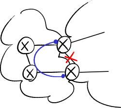 Partitioning of area 0.


The problem of partitioned areas is handled in OSPF differently depending on the type of area:
- edge area: the ABR does not summarize the information about all the networks present in the edge area, but only announces the networks which it is able to reach → packets toward the partition will be sent only to ABRs for which an internal path exists to arrive at the destination;
- area 0: OSPF is not able to automatically solve problems of partitioned areas in the backbone (the closest ABR is always chosen as the exit point), but in some cases the operator can manually enable between two ABRs a Virtual Link which physically crosses an edge area: when a packet arrives at an ABR, it goes back to the area going to the ABR at the other end of the tunnel and then at last enters area 0 → area 0 must always be logically, but not necessarily physically, contiguous.
Extending the backbone area[edit | edit source]

A link between two routers belonging to different edge areas normally can not be used: traffic from one area to another one in fact must always cross area 0.
Thanks to the Virtual Link it is possible to bring into the backbone a router in an edge area which is directly connected to a single backbone router: that internal router becomes an ABR to access area 0, and then all links connected to it can be used for traffic.
Metrics and costs[edit | edit source]
OSPF supports more than one metric simultaneously on a single link: the best path can be, depending on packets, for example
- the shortest path;
- the path with the best bandwidth capacity;
- the path with the lowest delay.
OSPF allows to define metrics depending on the 'Type of Service' (ToS) field in the IP packet → in theory, 64 types of service and then 64 different routing trees are possible, but in practice this feature is almost unused because the processing load required by the LS algorithm on each router would be duplicated for every ToS.
OSPF adopts equal-cost multipath routing. Differently from IGRP, OSPF does not define an unambiguous way to compute the cost of a link: the cost is assigned by the manufacturer of the network device → each manufacturer has its own default values, creating possible inconsistencies in multi-vendor networks → it is better to customize the cost values on the most important links (on both ends).
Router ID[edit | edit source]
Each OSPF router is uniquely identified by a Router ID, which is used as the 'name' for routers in OSPF packets (e.g. as the source in the OSPF header).
OSPF does not specify how the Router ID should be determined, but just specifies that it must be a 32-bit-long unique identifier. On Cisco devices, Router IDs can be obtained in two ways:
- manually: the network administrator explicitly configures the value of the Router ID (in IPv4 typically this is not done, while in IPv6 this is mandatory: B6. Instradamento IPv6#OSPFv3;
- automatically: an algorithm gets the Router ID from the IPv4 addresses of the router:
- if at least a loopback interface exists, the Router ID is equal to the biggest address among the ones of the loopback interfaces: loopback interfaces do not depend on the state of the physical interfaces and are thus more stable;
- if no loopback interfaces exist, the Router ID is equal to the biggest address among the ones of the OSPF network interfaces.
LSAs[edit | edit source]
Link State Advertisement (LSA) is the data structure, contained in Link State Update packets, which includes OSPF routing information:
- Router LSA: it describes an adjacency via a point-to-point link;
- Network LSA: it lists the routers attached to a transit network, and it is generated by the designated router of the transit network;
- Network Summary LSA: it contains the external routes inside other areas within the same OSPF AS (Summary Records), and it is generated by an ABR;
- ASBR Summary LSA: it notifies the location of the ASBR if it is not in area 0 but in an edge area;
- AS External LSA: it contains the external routes outside the OSPF AS (External Records), and it is generated by an ASBR.
Router LSA[edit | edit source]
- Adjacencies seen from router R1.
-
 Single router.
 -
 Router link.
 -
 Network link.


OSPF defines two types of link:
- router link (default): if there is a point-to-point link between two routers (e.g. serial interface), each of routers sees it as logically split into two point-to-point links:
- a point-to-point connection to the adjacent router, identified by its own Router ID;
- a point-to-point connection to the adjacent IP network, called stub network[1], that is the one which the network interface of the router belongs to.
If a router interface is enabled but is not attached to any other router, there is only the connection to the stub network (single router figure);
- network link (network link figure): if there is a broadcast network (e.g. Ethernet), called transit network, each of the two[2] or more routers attached to it sees it logically as a point-to-point connection to the adjacent transit network.
LSA Routers can describe several types of adjacencies via point-to-point links:
- adjacency to a router: it is generated by each of the two routers adjacent one to each other;
- adjacency to a transit network: it is generated by each of the routers adjacent to the transit network (including the designated router);
- adjacency to a stub network: it is generated by the router whose interface is adjacent to the stub network;
- adjacency to a Virtual Link: it is generated by each of the routers at the ends of the Virtual Link.
OSPF packets[edit | edit source]
All OSPF packets are directly encapsulated into IP (Protocol Type = 89), without any help from an intermediate transport protocol.
An OSPF header, the same for all packets, specifies the type of transported OSPF packet:
- type 1: Hello
- type 2: Database Description
- type 3: Link State Request
- type 4: Link State Update
- type 5: Link State Acknowledgement
Hello protocol[edit | edit source]
The hello protocol performs the fault detection without relying on the physical layer.
Hello packets are sent every HelloInterval (default = 10 s), and the adjacency is considered as disappeared and is no longer announced:
- as soon as the fault is detected at the physical layer;
- after a certain amount of lost Hello packets (default RouterDeadInterval = 40 s, equivalent to 4 Hello packets), if the fault can not be detected at the physical layer.
The LSA however remains in the OSPF database, and if not renewed it will expire after a period of time equal to MaxAge (default = 1 hour).
The Router ID is computed at the start of the OSPF process, and it is not modified even if the IP addresses on the router are modified → the router may appear with a different Router ID on reboot of the OSPF process (e.g. following a fault or a power outage) → in the topology computed by the LS algorithm a no longer existing node remains, until its LSA will expire.
Exchange protocol[edit | edit source]
The exchange protocol is used to perform the adjacency bring-up, that is to synchronize the database of two routers when they become adjacent.
The adjacency bring-up is performed only when needed, that is when a router has some not updated information in its database. Checking the need for a database update is performed:
- after a change in the network (e.g. at boot time or when a new link becomes active);
- whenever the LSA Refresh timer expires (default = 30 minutes), to refresh the ages of still valid LSAs before they expire.
During the adjacency bring-up, only old or missing LSAs are exchanged:
- Database Description: the master router sends the list of sequence numbers of all the LSAs in its database;
- Link State Request: the slave router sends the list of sequence numbers related to old or missing LSAs in its database;
- Link State Update: the master router sends the requested LSAs, and the Link State Update packet is propagated in selective flooding;
- Link State Acknowledgement: the slave router confirms it has received the Link State Update.
References[edit | edit source]
- ↑ The 'stub network' is not to be confused with the 'stub area'.
- ↑ OSPF does not prevent from configuring a point-to-point link between two routers as a transit network.
Inter-domain routing: peering and transit in the Internet
Traffic within the AS is almost 'free', excluding infrastructure costs (maintenance, administration, electricity, etc.) → ISPs try to convince users to spend most of their time inside the AS.
However, an AS should connect to other ASes for two reasons:
- an AS must be able to reach all the destinations present in the Internet for Metcalfe's law (= the network must be as more extended as possible to be useful);
- an AS would like to achieve resilience in its connections toward the outside world.
ASes on the Internet are interconnected by a hierarchical organization:
- Tier 1 (e.g. Seabone, Sprint): international operator interconnecting major towns by long-distance, broadband links and transporting big traffic flows along backbones;
- Tier 2 (e.g. Telecom Italia): national operator collecting traffic from single users through a lot of access points thanks to its house-to-house presence throughout the territory;
- Tier 3: local operator serving a very restricted geographical area.
Commercial agreements among ASes[edit | edit source]
Interconnections between an operator and another one may not come for free: usually, the interconnection between two ASes is established only upon an economic agreement. Two types of agreements are possible:
- transit: it represents the most natural choice from the economic viewpoint;
- peering: when two ASes discover that they can do better.
Inter-domain routing over the Internet is mainly driven by commercial agreements among operators at various hierarchical levels:
- Tier 1: it can advertise, independently of the geographical coverage of its network, the reachability of the full route (0.0.0.0/0), that is the reachability of (almost) every destination AS on the Internet, without having to buy transit from other providers or to pay some access fee;
- Tier 2: it needs to buy transit from a Tier-1 operator in order to be able to reach the whole Internet, and it can establish a lot of peering agreements with other Tier-2 providers;
- Tier 3: it has not any peering agreement, and simply buys transit from a Tier-2 (or Tier-1) provider.
Transit[edit | edit source]
An agreement is transit when an ISP has to pay another ISP to connect to its AS. The ISP receiving the money guarantees the 'transit', that is the right to use its network, to the traffic coming from the other AS.
The economic agreement may establish:
- the payment method:
- fee by volume: a maximum amount of bytes of data per day or per month, plus additional cost for traffic exceeding that amount;
- flat fee: a monthly fee for a maximum bandwidth (the bandwidth can be limited via software on the access interface).
- which destinations are reachable through the transit:
- full route: all destinations around the world must be reachable;
- only destinations in a certain geographical area (e.g. USA): packets directed toward other destinations are dropped.
The price may be influenced by the importance of the ISP selling the transit:
- an US ISP has control of the most important part of the network because inside its AS there are the most visited web servers in the world;
- a very large ISP can offer a good reachability with the rest of the world thanks to its high number of interconnections.
Peering[edit | edit source]
An agreement is peering when two peer ISPs agree to exchange traffic between themselves without having to pay each other.
Two ISPs can decide to stipulate a peering agreement if they determine that the costs for direct interconnection are lower than the costs for buying transit from each other: costs for setup and maintenance of the direct link between the ASes are equally split by the two ISPs, which can send data at the full speed allowed by the link.
Tier-1 operators work in a very competitive market:
- Tier-2 operators can establish new peering agreements among themselves as soon as they become more convenient than transit;
- a Tier-2 operator can shortly move to a more convenient Tier-1 operator;
- a dominant operator may be forced by the market guarantor to offer peering connections with minor ISPs.
Routing policies[edit | edit source]
In inter-domain routing, other requirements are more important than simple network connectivity:
- economic (who pays for the bandwidth?): sometimes longer paths may be preferred to best paths;
- administrative (is it allowed to go?): sometimes some paths are omitted to the other party;
- security (is that administrative domain trusted?): sometimes safer (and longer) paths may be preferred to best paths.
The path chosen by the routing protocol is not necessarily the least-cost path from the technical point of view, but it is the best path among the ones which satisfy the constraints established by routing policies configured by the network administrator, which reflect commercial agreements among ASes.
The decision process on border routers is affected by routing policies:
- routing table: the choice of some cheaper routes can be favoured and the choice of other ones across untrusted ASes can be discouraged;
- route advertisements: the routes announced toward other ASes may not correspond to the actual network topology.
Economic requirements[edit | edit source]

Sending traffic on a transit link costs → an AS can take advantage of a peering link, even if it is not a direct link, to make the other peer AS pay the transit cost (freeriding).
In the example in the side figure, two Italian ASes A and B are interconnected in peering, and each of them is connected in transit with US AS C. The best path according to the traditional routing rules is path x because it is made up of a direct link, but A needs to pay to make traffic go through that link. A can set a policy which prefers a cheaper path y: it deviates all the traffic directed to C to the link toward B, which is a low-cost link for A → B will send A's traffic to its transit link toward C, paying instead of A.
Administrative requirements[edit | edit source]

An AS can set a routing policy in order not to announce connectivity with other ASes to an AS (route hiding).
In the example in the side figure, B has a transit link toward C and uses it for its traffic, but advertises partial connectivity by omitting the information about this link in the advertisements which it sends to A, in order to avoid that A takes advantage of the peering link to save on the transit cost (and vice versa). A could not trust this advertisement and in turn set a policy forcing statically all traffic toward C to be sent to B anyhow → B can defend itself by setting an Access Control List (ACL) on its border router to discard all packets coming from A and directed toward C.
Security requirements[edit | edit source]

A network operator can represent a security threat because for example is used to make sniffing actions on traffic crossing its AS → an AS would like to avoid that its traffic directed to other ASes go through that untrusted operator.
In the example in the side figure, A to reach C prefers a longer but safer path x because it does not cross untrusted operator B, even if the latter is advertising low-cost path y toward C.
Internet Exchange Point[edit | edit source]
Interconnecting two ASes by direct connection, that is by a single wide-area link between them, is not convenient:
- link cost: its installation may require digging operations;
- cost of interfaces on routers: they have to send the signal over long distances;
- flexibility: intervention is necessary on the physical infrastructure to create a new interconnection.
An Internet Exchange Point (IXP) allows multiple border routers of different ASes (ISPs) to exchange external routing information in a more dynamic and flexible way.
Routers are connected through an intermediate data-link-layer Local Area Network: technically all routers are directly reachable, but in practice routing policies define interconnections according to commercial agreements among ASes → to create a new interconnection, it is sufficient to configure routing policies on single routers without having to change the physical infrastructure. An interconnection can also be active but used just as a backup (selection done in BGP).
Usually each AS pays a monthly fee, depending on the speed of the connection to the IXP. The IXP is in charge of the technical functioning of switches within the intermediate network:
- single location: often all routers are concentrated inside a room in a datacenter, where they are provided with:
- high-speed data-link-layer network;
- electrical power, conditioning system;
- monitoring service;
- proximity to optical-fiber backbones;
- distributed infrastructure: multiple access points are available in the main towns over the territory (for example, TOPIX runs across the entire Piedmont region).
The IXP is also known as Neutral Access Point (NAP): the IXP has to be neutral and uninvolved in its customers' business. An IXP can decide to disallow transit agreements: for example, MIX in Milan is a nonprofit organization which only admits peering agreements to favour internet diffusion in Italy, but this may limit the amount of traffic exchanged across the IXP because ISPs available only for transit agreements will choose other IXPs.
Network neutrality[edit | edit source]
Network neutrality is the principle according to which all traffic should be treated equally, without privileging or damaging a part of traffic for economic interests.
Network operators can be tempted to give 'preferential treatment' to portions of traffic:
- privilege some traffic: offer a better service for a certain kind of traffic (e.g. higher speed);
- damage some traffic: offer a worse service, or no service at all, for a certain kind of traffic.
A neutral network guarantees that all entities (e.g. content providers) have the same service, without making some service be killed at the discretion of the network operator, but enforcing 'pure' network neutrality implies that traffic control, which may be useful in many cases, is not possible at all; on the other end, if it is admitted that the network may not be neutral, the network operator is given the power to privilege some traffic or content. In an open market the ball is leaved to the user: if users do not agree that their VoIP traffic is discriminated, they can switch to another network operator (although in practice this may not always be possible due to cartels among network operators).
- Examples of non-neutrality
- content providers: ISPs would like to have a part of revenues of content providers → an ISP may privilege traffic directed to a content provider with which it stipulated a revenue sharing agreement;
- peer-to-peer (P2P):
- end users do not care about destination of their traffic, but P2P traffic can reach every user in every AS around the world making the ISP pay high costs → an ISP may privilege traffic which is generated within the AS (e.g. AdunanzA by Fastweb);
- P2P traffic is more symmetric because it uses a lot the upload bandwidth, while networks have been sized to support asymmetric traffic → an ISP may privilege asymmetric traffic (e.g. normal web traffic);
- quality of service (QoS): an ISP may privilege traffic with a higher priority level (e.g. VoIP traffic);
- security: an ISP may block traffic from malicious users (e.g. DDoS attack).
Border Gateway Protocol
Border Gateway Protocol (BGP) is the inter-domain routing protocol commonly used in the Internet.
- Overview
- it uses the Path Vector (PV) algorithm to record the sequence of ASes along the path without the risk of routing loops: #Path Vector algorithm;
- routers can aggregate the received routing information before propagating them: #Route aggregation;
- it does not automatically discover the existence of new neighbor routers, but peering sessions must be configured by hand: #Peering sessions;
- it exchanges routing updates by using reliable TCP connections: #TCP;
- it is an extensible protocol thanks to the Type-Length-Value (TLV) format of attributes: #Path attributes;
- it supports routing policies: #Decision process.
Routing information[edit | edit source]
BGP exchanges inter-domain routing information about external routes, which are in form network address/prefix length (instead of the netmask).
Path Vector algorithm[edit | edit source]
As routing policies are defined based on paths, BGP can not be based on the DV algorithm because it is not enough to know their costs. BGP chooses to adopt the Path Vector (PV) algorithm: every AS constitutes a single node, identified by a number of 2 (or 4) bytes, and the additional piece of information is the \ul{list of crossed ASes}.
The PV algorithm is more stable because it is easy to detect loops:
- if a router receives a PV which already includes its AS number, it discards the PV without propagating it, because a routing loop is going to start;
- otherwise, the router enters its own AS number into the PV and then it propagates it to its neighbors.
BGP does not support an explicit cost metric: the cost associated to each route is simply equal to the number of crossed ASes included in the list → the least-cost route may not be the actually optimal one:
- ASes may have different requirements, hence they may adopt different metrics one from each other (e.g. bandwidth, transmission delay) → it is difficult to compute coherent costs for all ASes;
- the announced cost may not match the actual network topology because an ISP may want to hide from a competitor the actual information about its own network for economic reasons: B4. Inter-domain routing: peering and transit in the Internet#Administrative requirements.
Route aggregation[edit | edit source]
When a border router propagates information about received routes, it can be manually configured to include aggregate routes into its advertisement messages to reduce their size: two routes can be aggregated in a route with the common part of their network prefixes.
However not all the routes which has been collapsed into an aggregate route can have the same sequence of crossed ASes, but there could be a more specific route following another path:
- overlapping route: also the specific route, with its different list of crossed ASes, is announced along with the aggregate route → information is complete, and the 'longest prefix matching' algorithm will select the more specific route in the routing table;
- not precise route: only the aggregate route is announced → information is approximate, because the list of crossed ASes does not match the path actually followed for all the destination addresses within that address range.
Peering sessions[edit | edit source]
Two border routers exchanging BGP messages between themselves are called peers, and the TCP-based session is called peering session.
A key difference compared to other routing protocols is the fact that peers are not able to discover each other automatically: manual configuration by the network administrator is required, because peers may not be connected through a direct link but other routers, for which BGP updates are normal data packets to be forwarded to destination, may exist between them.
TCP[edit | edit source]
Transmission of routing information is reliable because two peers establish a peering session by setting up a TCP connection through which all BGP messages are exchanged:
- existing components are reused instead of redefining yet another protocol-specific mechanism;
- BGP does not need to deal directly with retransmissions, lost messages, etc.
Using TCP as transport protocol avoids to periodically send updates: an update is sent only when needed, including just routes which have changed, and it is sent again only if the message went lost → the bandwidth consumed to send routes is reduced.
Since advertisements are not periodic, routes never expire → it is required to explicitly inform that a previously announced route has become unreachable, to withdraw routes when they are no longer valid (analogously to route poisoning in the DV algorithm.
However TCP deprives the application of the control on timings, because control packets may be delayed by TCP mechanisms themselves: in case of congestion TCP reduces the transmission bit rate preventing their timely transmission → quality of service can be configured on internal routers within the AS so as to give priority to BGP packets, considering that they are service packets to allow the network operation.
TCP does not provide any information about whether the remote peer is still reachable → an explicit keepalive mechanism managed by BGP itself is required. Also keepalive messages rely on TCP mechanisms → reactivity to a peer disappearance or a link fault is limited, but it is still acceptable considering that these events are rare (e.g. links between border routers are strongly redundant).
I-BGP e E-BGP[edit | edit source]
When two border routers set up a peering session between themselves, each one communicates, through an OPEN message, its AS number to the other party to determine the type of sub-protocol:
- Exterior BGP (E-BGP): peers are border routers belonging to two different ASes, usually connected by a direct link;
- Interior BGP (I-BGP): peers are border routers belonging to the same AS, usually connected through a series of internal routers.
The processing of BGP messages and the routes announces on peering sessions may be different according to which ASes the peers are belonging to:
- E-BGP: when a border router propagates a PV to an E-BGP peer, it prepends the current AS number to each list of crossed ASes:
- external routes: they are propagated to other E-BGP peers, but peers whose AS is on the best path toward those destinations;
- internal routes: they are propagated to other E-BGP peers;
- I-BGP: when a border router propagates a PV to an I-BGP peer, it transmits the list as is because the AS number remains unchanged:
- external routes: they are propagated to other I-BGP peers according to various ways;
- internal routes: they are never propagated to other I-BGP peers, but every border router learns them from an independent redistribution process.
I-BGP sessions are used to exchange external routes:
- independently of routes exchanged by the interior protocol: the direct connection between peers avoids to bother the IGP protocol when the variation of an external route does not require the re-computation of internal routes → no transients, less processing;
- independently of the interior protocol: if border routers when learning external routes from E-BGP limited to redistribute them to the IGP protocol, letting the latter redistributed them naturally to other border routers, some important information needed by BGP would go lost → specific BGP messages, called UPDATES, are required, including this information in their attributes.
IGP-BGP synchronization[edit | edit source]

BGP routers in a transit AS learn external destinations by other BGP routers via I-BGP, but packet forwarding across the AS (toward the egress BGP router) relies on internal routers, whose routing tables are filled by the IGP protocol and not by BGP → only after they have been announced also by the IGP protocol, external destinations can be announced to border routers in other ASes.
In the example in the side figure, router R4 learns destination D via E-BGP and announces it to router R3 via I-BGP, but R3 can not in turn announce it to router R5 via E-BGP until the destination is redistributed from the IGP protocol to R3, otherwise if R5 tried to send a packet toward D, R3 would forward it inside the AS where internal routers would discard it.
It might be good to disable synchronization when:
- the AS is not a transit one;
- all routers in the AS use BGP.
Routing loops[edit | edit source]

Lack of information about crossed border routers when they belong to the same AS can be the cause of routing loops: a border router can no longer rely on the list of crossed ASes to detect paths going twice through the same border router.
In the example in the side figure, a loop is created in advertising:
- router R4 learns the external route toward destination D;
- R4 propagates D to peer R3;
- R3 propagates D to peer R2;
- R2 propagates D to peer R4, which is the router which first learnt and announced D.
Thus a situation is created similar to the one which was triggering count to infinities in the Distance Vector algorithm: R4 can not determine whether R2 can reach D by crossing R4 itself or an actually alternative path exists → if a link fault occurs between R4 and the border router of the AS where D is located, R4 will believe that D is still reachable through R2.
External routes can be announced to I-BGP peers in various ways: full mesh, route reflector, AS confederation.
Full mesh[edit | edit source]

Each border router has an I-BGP peering session with every other border router of its AS.
When a border router learns an external route from E-BGP, it propagates it to all other ones, which in turn propagate it to everyone, and so on.
In presence of more than 2 border routers, routing loops can form due to loops in advertising, like in the side figure.
This solution is not flexible because all peering sessions must configured by hand, although peering sessions do not change much over time because border routers are quite fixed and fault-tolerant.
Route reflector[edit | edit source]

One of the border routers is elected as the route reflector (RR), and all other border routers set up peering sessions only with it without creating closed paths.
When a border router learns an external route from E-BGP, it propagates it only to RR, which is in charge of in turn propagate the route to other border routes avoiding routing loops.
Route reflector constitutes a single point of failure.
AS confederation[edit | edit source]

Border routers have a full mesh of I-BGP peering sessions (as in the first way), but the AS is split into mini-ASes, each one with a private AS number, and when a border router propagates the PV it prepends in the list its private AS number.
When an advertisement arrives, the border router can look whether its own private AS number is already in the list, so as to discard the packet if a routing loop is detected.
Path attributes[edit | edit source]
BGP information about announced routes (e.g. the list of crossed ASes) is included in path attributes inside UPDATE packets.
All attributes are encoded into the Type-Length-Value (TLV) format → BGP is an extensible protocol: extension RFCs can define new attributes without breaking compatibility with the existing world and, if the router does not support that attribute (unrecognized type code), it can ignore it and skip to the next one (thanks to the information about its length).
A BGP attribute can be:
- well-known: it must be understood by all implementations, and can never be skipped:
- mandatory: it must be present in all messages;
- discretionary: it may not be present in all messages;
- optional: it may not be understood by all implementations, and can be skipped if not supported:
- transitive: if the router does not support the attribute, it must propagate it anyhow setting flag P;
- non-transitive: if the router does not support the attribute, it must not propagate it.
Each attribute has the following TLV format:
| 1 | 2 | 3 | 4 | 8 | 16 | 24/32 | |
| O | T | P | E | 0 | Type | Length | Value |
where the fields are:
- Optional (O) flag (1 bit): it specifies if the attribute is optional or well-known;
- Transitive (T) flag (1 bit): it specifies if the attribute is transitive or non-transitive;
- Partial (P) flag (1 bit): it specifies if at least a router along the path has encountered an optional transitive attributed which did not support;
- Extended Length (E) flag (1 bit): it specifies if the 'Length' field is encoded by one of two bytes;
- Type field (1 byte): it includes the type code identifying the attribute → a router can determine if it supports that attribute without having to parse its value;
- Length field (1 o 2 bytes): it includes the length of the attribute value → a router can skip an unsupported attribute and skip to the next one by advancing by the number of bytes indicated by this field;
- Value field (variable length): it includes the attribute value.
Well-known attributes[edit | edit source]
- ORIGIN attribute (type 1, mandatory): it defines the origin of the path information:
- IGP: the route was manually specified as a static route (bgp network command);
- EGP: the route was learnt by the EGP protocol[1];
- INCOMPLETE: the route was learnt from an IGP protocol through a redistribution process (bgp redistribute command);
- AS_PATH attribute (type 2, mandatory): it contains the list of crossed ASes split into path segments:
- AS_SEQUENCE: AS numbers in the path segment are in traversal order, and if the first segment in the packet is in order a new AS number has to be added at the beginning of that segment;
- AS_SET: AS numbers in the path segment are not in traversal order, and if the first segment in the packet is not in order a new in-order segment, where the new AS number has to be inserted, has to be added before that segment;
- NEXT_HOP attribute (type 3, mandatory): it optimizes routing when multiple routers belong to the same LAN but to two different ASes, and therefore traffic from an AS to another one would always cross the border router → the border router can announce to send traffic to the next hop router in the other AS:

- LOCAL_PREF attribute (type 5, discretionary): in I-BGP when the external destination is reachable across two egress border routers, the route with highest LOCAL_PREF is preferred;
- ATOMIC_AGGREGATE attribute (type 6, discretionary): it indicates that the announced route is a not precise aggregate route.
Optional attributes[edit | edit source]
- MULTI_EXIT_DISC (MED) attribute (type 4, non-transitive): in E-BGP when two ASes are connected via multiple links, the link with lowest MED is preferred and links with higher MEDs are considered as backup links;
- AGGREGATOR attribute (type 7, transitive): it contains the AS number and the IP address of the router which generated the not precise route;
- COMMUNITIES attribute (type 8, transitive): it indicates which group of peers this route has to be announced to (e.g. to the entire Internet, only within the current AS, to no one);
- MP_UNREACH_NLRI attribute (type 15, non-transitive): it informs that a previously announced route has become unreachable (routes never expire).
Decision process[edit | edit source]

The decision process running on every border router is responsible for:
- selecting which routes are advertised to other BGP peers;
- selecting which routes are used locally by the border router;
- aggregating routes to reduce information.
Databases which BGP has to deal with are:
- Routing Information Base (RIB): it consists of three distinct parts:
- Adjacent RIB Incoming (Adj-RIB-In): it contains all the routes learnt from the advertisements received from a certain peer;
- Local RIB (Loc-RIB): it contains the routes selected by the decision process with their degree of preference;
- Adjacent RIB Outgoing (Adj-RIB-Out): it contains the routes which will be propagated in advertisements to a certain peer;
- Policy Information Base (PIB): it contains the routing policies defined by manual configuration;
- routing table: it contains the routes used by the packet forwarding process.
Very complex routing policies can be imposed to affect the decision process:
- a certain function returning, by applying the policies defined on attributes, the degree of preference for that route is applied to each route in the Adj-RIBs-In.
Policies are defined only based on the attributes of the current route: the computation of the degree of preference is never affected by the existence, the non-existence, or the attributes of other routes; - for each destination, the route with the greatest degree of preference is selected and inserted into the Loc-RIB;
- other policies determine which routes are selected from the Loc-RIB to be inserted into the Adj-RIBs-Out.
References[edit | edit source]
- ↑ The protocol, not the protocol class, is meant here.
IPv6 routing
Nowadays routers are mostly ready for IPv6, even though performance in IPv6 is still worse than the one in IPv4 because of lack of experience and lower traffic demand. Often IPv6 routing is turned off by default even if the device supports IPv6 (on Cisco routers this is enabled by command ipv6 unicast-routing).
Two aspects have to be considered:
- routing tables: how to handle the forwarding of data packets?
- routing protocols: how to distribute routes across the network?
Routing tables[edit | edit source]
Routing in IPv6 is performed in the same way as IPv4 but it requires two distinct routing tables, one for IPv4 routes and another for IPv6 routes. IPv6 routing tables can store several types of entries, including:
- indirect entries (O/S codes): they specify the addresses, typically link local, of the interfaces of the next-hop routers to which to send packets addressed towards remote links;
- direct entries: they specify the interfaces of the router itself through which to send packets addressed towards local links:
- connected networks (C code): they specify the prefixes of the local links;
- interface addresses (L code): they specify the interface identifiers in the local links.
Next hop[edit | edit source]
As the next hop in computed dynamic routes, routing protocols always use link local addresses, even if a global address is configured on the neighbor interface, for the sake of simplicity: link local addresses always exist, while global addresses may not be used in some portions of the network.
However the usage of link local addresses makes difficult the task of determining the location of that address: the network address of a global address at least allows to identify the network in which the host should be present and thus determine the output interface, but a link local address that begins with FE80:: can be everywhere → next to the next hop address, routers also print the output local interface to solve ambiguities, such as:
For static routes, the choice is left to the network manager, who can use the address he prefers as the next hop:
- broadcast interface (e.g. Ethernet): the address of the next hop needs to be specified:
- global address: the local interface does not need to be specified because it can be determined from the network prefix:
ipv6 route 2001:1::/64 2001::1
- link local address: the local interface needs to be specified too to identify the scope of the link local address:
ipv6 route 2001:1::/64 FastEthernet0/0 fe80::1
- global address: the local interface does not need to be specified because it can be determined from the network prefix:
- point-to-point interface (e.g. serial): the address of the next hop does not need to be specified because it is uniquely identified by the local interface:
ipv6 route 2001:1::/64 serial 0
Since static routes can not adapt to network changes, it is strongly recommended to use global addresses as the next hop for static routes. This avoids that a route becomes invalid if the next hop changes: for example, if the network card on the next hop router is replaced because of a hardware fault:
- link local address: it depends on the MAC address of the card → the route needs to be changed;
- global address: the new interface should just be assigned the same global address.
Routing protocols[edit | edit source]
Routing protocols supporting IPv6 can adopt two approaches:
- integrated routing (IS-IS, MP-BGP4): the protocol allows to exchange both IPv4 and IPv6 routing information at the same time:
- efficiency: IPv4 and IPv6 addresses belonging to the same destination can be transported via a single message;
- flexibility: a single protocol transports multiple address families;
- reactivity: if a fault or a network change occurs, the protocol discovers it for both address families;
- bugs: a problem in the protocol affects IPv4 and IPv6 networks in the same way;
- migration: if the protocol uses IPv4 to transport Hello packets, IPv4 can not be abolished in the network;
- ships in the night (RIPng, EIGRP, OSPFv3): the protocol allows to exchange only IPv6 routing information:
- efficiency: given a destination, a message needs to be exchanged for its IPv4 address and another message for its IPv6 address, and the messages are completely independent of each other;
- flexibility: two different protocols can be used, one for IPv4 routing information and another for IPv6 routing information;
- reactivity: if a fault or a network change occurs, both protocols have to discover it, each one with its timings and duplicate messages;
- bugs: a problem in the protocol does not affect routing in the other one;
- migration: each routing protocol generates messages of the address family it belongs to.
RIPng[edit | edit source]
RIPng adopts the 'ships in the night' approach, and makes improvements to RIP mainly in Cisco command-line interface:
- support for multiple instances: the tag field allows to specify the protocol instance;[1]
- per-interface configuration: new commands have been introduced:
- ipv6 rip <tag> enable: it replaces the network command and automatically configures RIP on that interface without having to specify an address;
- ipv6 rip <tag> default-information originate: it originates the default route (::/0), that is the rest of the world can be reached via this interface.
OSPFv3[edit | edit source]
OSPFv3 adopts the 'ships in the night' approach, and differs from OSPF mainly for three aspects:
- per-interface configuration: the ipv6 ospf <process ID> area <area ID> has been introduced which specifies that all the networks and the addresses configured on this interface will be advertised as belonging to the specified area;
- Router ID: unfortunately OSPFv3 still uses a 32-bit-long Router ID, which it is not even able to automatically set when no IPv4 addresses is available → the ipv6 router-id <number> command becomes compulsory when the router is IPv6-only or is in an IPv6-only network;
- tunnel: a IPv6-on-IPv4 tunnel can be configured to connect together IPv6 islands through an IPv4 network.
IS-IS[edit | edit source]
IS-IS for IPv6 adopts the 'integrated routing' approach: in fact it uses its own layer-3 protocol to transport protocol-specific packets, independently of the underlying IP protocol version.
MP-BGP4[edit | edit source]
MP-BGP4 can adopt both approaches depending on configuration: TCP packets can be enveloped into IPv4 or IPv6 as needed.
The most common deployment follows the 'integrated routing' approach, because of the need to use the AS number (which is the same for both IPv4 and IPv6) for the BGP process. Integration also reflects to policies: IPv4 addresses and IPv6 addresses can be mixed at will.
References[edit | edit source]
- ↑ Support for multiple instances was already present in RIPv2, but was not configurable on Cisco routers.
Multicast routing2
- Multicast routing protocols
- DVMRP: DV (TRPB, RPM), unicast-protocol-independent, source-specific tree;
- MOSPF: LS, works on OSPF protocol, source-specific tree;
- PIM-DM: DV (RPM), unicast-protocol-independent, source-specific tree;
- PIM-SM: CBT, unicast-protocol-independent, hybrid between shared and source-specific tree;
- BGMP: BGP-based inter-domain multicast routing protocol.
DVMRP[edit | edit source]
Distance Vector Multicast Routing Protocol (DVMRP) was the first multicast routing protocol, and was used at the origins in Multicast backbone (Mbone), a virtual network born in 1992 in the IETF scope which relies for transmission on the same physical structure as the Internet to provide users with the possibility to exploit multicast for multimedia communications.
DVMRP is based on the DV algorithm:
The DVMRP protocol instance is run in parallel with the unicast protocol instance: DVMRP ignores routing information from other protocols, and computes routes which can differ from the ones used for unicast traffic.
It uses a metric based on the hop count, that is the number of mrouters which speak DVMRP. In DVMRP tunnels can be manually configured: the path connecting two DVMRP neighbors can include routers not supporting DVMRP (or on which DVMRP is disabled):
- local end-point: it specifies the mrouter at the beginning of the tunnel;
- remote end-point: it specifies the mrouter at the other end of the tunnel;
- metric: it specifies the cost measure of the tunnel;
- threshold: it specifies the minimum TTL value which a packet needs to have in order to be routed through the tunnel → it allows to define the packet visibility: packets which must not exit the corporate network are generated with a TTL equal to the threshold.
MOSPF[edit | edit source]
Multicast OSPF (MOSPF) is a multicast routing protocol based on the LS algorithm which extends OSPF, enabling single routers to have a full knowledge of the network topology and costs related to single links.
MOSPF is backward-compatible with OSPF: MOSPF routers can be mixed with OSPF-only routers, although multicast packets are forwarded only among MOSPF routers and the paths chosen for multicast packets do not cross OSPF-only routers.
MOSPF adds LSA type 6:
- MOSPF internal routers produce LSAs type 6 to inform the other routers within their area of multicast groups being active on their networks;
- MOSPF ABRs produce LSAs type 6 to inform the other routers within area 0 of multicast groups being active on their edge areas (even by aggregation).
PIM[edit | edit source]
Protocol Independent Multicast (PIM) directly uses tables containing routing information independently of the underlying unicast protocol (DV or LS) which has built them.
It exists in two versions, incompatible among them, dealing with different issues related to spatiality of receivers:
- Dense Mode (DM):
- it is suitable for small networks (LAN/MAN) with a lot of concentrated receivers;
- it is greedy in terms of bandwidth: packets can be forwarded to areas not interested in the particular multicast group;
- it adopts the DV-based RPM algorithm (like DVMRPv3);
- Implicit Join Protocol: in the absence of explicit Prune messages, packets are forwarded to a certain network;
- Prune messages should be generated to stop multicast traffic (like DVMRP);
- Sparse Mode (SM):
- it is suitable for wide networks (WAN) with few scattered receivers;
- it limits as much as possible the bandwidth overhead: it never uses flooding;
- it is an evolution to the CBT algorithm: it always starts from a shared tree, which becomes a source-specific tree when advantageous;
- Explicit Join Protocol: in the absence of explicit Join messages, packets are not forwarded to a certain network (routing information however goes to all routers, not only the ones which will receive traffic);
- Join messages should be generated to start multicast traffic (like MOSPF).
PIM-SM[edit | edit source]
PIM-SM handles two kinds of distribution trees:
- RP-Tree (RPT): it is the shared tree used at the beginning for all the packets of the multicast group, but is not optimized based on the source → the first packets of the transmission can be delivered in a short time to receivers without having to wait for the tree computation:
- no shortest paths are used;
- traffic is centralized;
- one tree is corresponding to each multicast group;
- Shortest-Path Tree (SPT): it is the source-specific tree built at a later time if routers believe it is convenient (it is not mandatory):
- shortest paths are used;
- traffic is distributed;
- one tree is corresponding to each (group, source) pair.
PIM-SM defines three special nodes:
- rendez-vous point (RP): it is the core router, elected based on an algorithmic formula starting from a list called RP-set, which is in charge of:
- receiving Join messages by DRs;
- receiving registration requests by sources;
- receiving and sending to DRs the first multicast data packets transmitted by a source;
- designated router (DR): it is the router, elected based on the shortest path toward the RP (or on the higher IP address if there is a tie), which is in charge of:
- receiving subscription requests by hosts in a certain LAN;
- sending the Join message to the RP to join the RPT;
- sending the Join message to the source to join the SPT;
- sending the Join message periodically to adapt to group changes;
- bootstrap router (BSR): it is the router, elected based on the best administrative cost (or on the higher IP address if there is a tie), which is in charge of distributing the RP-set to the whole PIM-SM domain.
Algorithm[edit | edit source]
- RPT
- subscription of DRs as receivers: each DR sends a Join message to the RP;
- registration of the source as a transmitter: the source sends a registration request to the RP;
- registration of the RP as a receiver: the RP sends a Join message to the source;
- transmission along the RPT: the source sends in multicast the first data packets, forwarded by intermediate routers up to the RP;
- propagation along the RPT: the RP propagates in multicast the received data packets, forwarded by intermediate routers up to the DRs.
- SPT
- subscription of DRs as receivers: each DR sends a Join message to the source;
- transmission along the SPT: the source sends in multicast data packets, forwarded by intermediate routers to each DR (besides the RP);
- detachment from the RPT: each DR sends a Prune message to the RP;
- joining to the SPT: another DR sends a Join message to the RP, then sends a Join message to the source.
Content Delivery Networks
A web cache is a device that stores a local copy of most recently required content (e.g. HTTP resources) and reacts as a proxy server to clients' requests:
- the web cache is closer to the user with respect to the web server:
- performance: the reply is faster when the requested resource is already in cache;
- bandwidth: expensive long-distance links (e.g. transoceanic links) are not loaded;
- reactive solution: if the requested resource is not in cache, the user needs to wait for the web cache to acquire (pull) it from the web server;
- no transparency: the user's web browser needs to be manually configured to contact that web cache.
A Content Delivery Network (CDN) is an overlay network[1] of web caches scattered all around the world but cooperating with the purpose of offering to the user a better quality of experience[2]:
- proactive solution: the web server copies (push) content (generally the most popular one) to the web cache before the users will ask for it;
- transparency: the user connects to the web cache automatically, without the need for manual configuration on his own client;
- performance: the user, even if he moves, always connects to the closest web cache;
- load balancing: the user always connects to the least loaded web cache;
- scalability: the content deployment into multiple replicas allows a large number of requests which a single web server alone would not be able to serve;
- conditional access: it is possible to customize returned content based on the user (e.g. targeted advertisements).
CDNs are ideal for content generating large amounts of traffic (e.g. multimedia resources), but not all content can be cached:
- dynamic web pages (e.g. stock market prices);
- customized-content web pages (e.g. user account).
CDNs can be deployed in a variety of ways:
- DNS-based CDNs: traffic is redirected to the best replica based on host names:
- DNS-based routing: the hosting provider needs to enter into agreements with DNS server managers;
- Akamai approach: intervention on DNS servers is not needed;
- URL-based CDNs: traffic is redirected to the best replica based on full URLs:
- server load balancing: the TCP connection termination point is close to the server;
- content routing: the TCP connection termination point is close to the client.
DNS-based CDNs[edit | edit source]
DNS-based routing[edit | edit source]


Selection of the best replica takes place when the host name is translated to an IP address. The DNS reply to a query does not depend only on the host name, but also on the source: a special DNS server computes, based on as many metrics as possible (RTT, server load, response time, etc.), a replica routing table containing entries like:
{host name, client IP address} → replica IP address
The routing engine in the 'modified' DNS server has a standard interface to guarantee transparency: the user believes that the IP address corresponding to the host name is the IP address of the real web server, while it is the IP address of one of its replicas.
Adding a new actor, the hosting provider, constitutes a new business opportunity in the network world:
- access provider: it provides network access to users;
- backbone provider: it provides long-range connectivity;
- hosting provider: it provides the CDN service to content providers;
- content provider: it provides content.
- Issues
- metrics: metric measurement, especially the dynamic ones, is not easy, and layer-3 metrics alone are not particularly meaningful;
- DNS caching: only the authoritative server knows all replicas and can select the best replica based on the client location → intermediate DNS servers in the hierarchy can not cache DNS replies;
- granularity: redirection granularity is at host-name, not single-URL, level → content of large web sites can not be split into multiple caches, hence the same replica will be asked for two different pages in the same web site.
Akamai approach[edit | edit source]
Akamai CDN exploits a proprietary automatic algorithm to redirect traffic to its replicas without any intervention on DNS servers:
- the user types the address of a web page with its normal domain name (e.g. http://cnn.com/index.html);
- the server of the content provider (e.g. CNN) returns a web page where the address of every multimedia resource (e.g. image) has a special domain name corresponding to a specific replica on an Akamai cache (e.g. http://a128.g.akamai.net/7/23/cnn.com/a.gif instead of http://cnn.com/a.gif);
- the user's web browser when parsing the page performs DNS queries to the new domain names and gets multimedia resources from the closest replicas.
URL-based CDNs[edit | edit source]
Server load balancing[edit | edit source]

The real servers containing replicas are seen by clients as a single virtual server with the same IP address.
The traffic load destined to the virtual server is balanced among the several real servers by a Server Load Balancer (SLB):
- layer-4 switching: TCP connections are not terminated by the SLB (content-unaware):
- one of the real servers answers the three-way handshake with the client;
- all HTTP queries belonging to the same TCP session have to be always served by the same real server;
- load balancing can be based on the source IP address, the source TCP port, etc.;
- layer-7 switching: TCP connections are terminated by the SLB (content-aware), acting as a proxy:
- the SLB answers the three-way handshake with the client, to be able to catch URLs requested at a later time;
- each HTTP query can be served by the currently least loaded real server, based on SLB decisions;
- load balancing is based on the full URL.
- Issues
- encrypted connections (HTTP): the SLB needs to have the private SSL cryptographic key of the server, and needs to support the processing load for encrypting/decrypting packets in transit;
- sticky connections: some applications require that TCP connections from the same client are redirected to the same server (e.g. shopping cart) → cookies should be considered too;
- geographical distribution: all replicas are close to each other and to the SLB, which is far away from the client.
Content routing[edit | edit source]
Content routers are routers which route traffic based on the URL toward the best replica:
- TCP: all content routers in a sequence terminate TCP connections between them → too many delays are introduced;
- content delivery control protocol: the URL is extracted by the first content router, and is propagated by a specific protocol.
- Issues
- stateful: the first content router needs to terminate the TCP connection to be able to catch the URL the user will query;
- complexity of devices: packet parsing for getting the URL is complex → layer-7 switches are complex and expensive devices;
- complexity of protocols: proposed content delivery control protocols are really complex;
- privacy: content routers read all the URLs queried by users.
References[edit | edit source]
- ↑ An overlay network is a computer network which is built on the top of another network.
- ↑ Quality of experience is a measure of a user's experiences with a service (e.g. web browsing).
Hints on the architecture of network devices
The architecture of routers has been evolving over time to increase more and more their packet processing capability:
- first generation (until early 1990): lower than 500 Mbps;
- second generation (early 1990): about 5 Gbps;
- third generation (late 1990): starting from 50 Gbps;
- multi-chassis (recent trend): of the order of Tbps.
First generation[edit | edit source]

First-generation routers were basically modified PCs:
- network interfaces: they are normal NICs, in a greater number and in manifold kinds with respect to the ones on a normal PC;
- memory: solid-state memory (e.g. SD card) is preferred because less subject to failures with respect to a mechanical hard disk;
- operating system: it is optimized specifically for network traffic processing.
- Advantage
- economy of scale: it uses components manufactured on a large scale instead of components dedicated to networking world.
- Disadvantages
- bottlenecks:
- shared bus:
- slow path: each packet transits twice over the bus;
- arbitrage: one NIC at a time can use the bus → multiple interfaces can not work in parallel;
- memory access: the routing table is stored in a data structure in the generic memory → accesses are not so localized as in traditional PCs, and the cache is little used;
- processing capability: the CPU interrupts the operating system whenever a packet arrives;
- shared bus:
- network interfaces: traditional network cards have not many ports and only support the most common kinds of interfaces;
- maintenance costs: using open-source components (e.g. PPP client) brings integration troubles and varied configuration ways.
Currently this architecture is used for mid-low-end routers, whose performance is adequate for small offices.
Second generation[edit | edit source]

Second-generation routers try to solve the performance problem by moving the processing load from the core CPU to edge units: NICs are replaced by line card, 'smart' network cards which add forwarding modules to physical/MAC components:
- CPU: the packet processor is a dedicated processor for 'simple' packet processing;
- memory: each incoming packet is stored into a local memory split from the one (generally TCAM) containing the routing table;
- routing table: sometimes the updated routing table is copied from the central unit to line cards.
Packets can follow two ways:
- fast path: the packets falling in the typical case (e.g. IPv4) transit only once over the bus: they are processed directly by the packet processor and are immediately sent to the output interface;
- slow path: least frequent packets (e.g. IPv6, OSPF) are leaved to the core CPU for a more sophisticated processing, at the cost of a definitely lower throughput.
The work of line cards should be coordinated by the core CPU, on which routing protocols (e.g. OSPF) are running too, which is mounted on a card called supervisor in high-end systems.
- Advantages
- core CPU: it works only for packets along the fast path → it can be less powerful;
- fast path optimization: the first packets in a connection follow the slow path, then the central system marks the connection as eligible for the fast path and all following packets will follow the fast path;
- flexibility: the introduction of a new protocol (e.g. IPv6) only requires updating the software on the central system.
- Disadvantage
- shared bus arbitrage: one line card at a time can use the bus → multiple interfaces can not work in parallel.
Third generation[edit | edit source]

Third-generation routers focus on the word parallelization problem by replacing the shared bus with a switching fabric (or crossbar) able to handle multiple transfers: a line card is connected to another line card by shorting the switch at the intersection of their 'wires' in the switching matrix.
Two line cards can not be connected to another same line card at the same time → an arbiter is needed which drives switching points and solves contention situations without collisions.
When output interfaces are slow in sending packets with respect to the switching speed of the switching fabric, packets can be queued in various ways:
- output queuing: buffers are placed on output interfaces → worst case: switching fabric N times faster than receiving speed, with N = number of input interfaces;
- input queuing: buffers are placed on input interfaces → the switching speed of the switching fabric does not depend on the number of input interfaces, but suffers from the head-of-line blocking problem:
- two packets in two input queues are destined to the same output queue;
- the arbiter lets one of the packets pass blocking the other one;
- all the following packets in the input queue, even the ones destined to free output queues, have to wait for the 'head of line';
- virtual output queuing: it solves the head-of-line blocking problems by keeping one queue per output at each input;
- buffered fabric: buffers are placed inside the crossbar at the spot of switching nodes.
- Disadvantages
- arbiter:
- it constitutes a bottleneck, especially in case of frequent decisions due to small packets (e.g. ATM);
- scheduling policies for quality of service may make its hardware more complex;
- queue buffers: they are expensive memories because they should be fast.
Multi-chassis routers[edit | edit source]
Multi-chassis routers aim at scalability: multiple flanked racks are connected so as to appear as a single router:
- the processing power is multiplied by the number of chassis;
- there is more physical room for network interfaces → a large number of links can be connected to a same device;
- routing is concentrated in a single station (like in the telephone world) instead of a lot of small routers spread over the network → the data station can serve all the users within a wide geographical area (e.g. Piedmont).
Service cards[edit | edit source]
Another recent trend aims at flexibility: routers are no longer purely layer-3 devices, because a lot of other features not belonging to layer 3 are being added, such as cache, firewall, network monitor, ACL, etc. The goal is to customize the service offered by ISPs, bringing back a portion of the business currently in the hands of content providers.
A currently common solution are service cards, line cards enriched with value-added services pre-configured by the manufacturer. Service cards however are not so flexible: being not programmable, a new service card should be purchased to add a service.
Major current issues[edit | edit source]
Throughput is no longer a current issue by now, but the current major issues are:
- purchase costs: to reduce the cost of network devices dedicated components are being replaced by general-purpose components made on a large scale:
- mainstream CPUs have too short product life cycles and too long replacement times → Intel recently proposed embedded CPUs with longer product life cycles and shorter replacement times with respect to mainstream CPUs;
- in dedicated systems the programmer could exploit the memory hierarchy, by storing the RIB into a slow memory and the FIB into a fast memory (e.g. TCAMs), while general-purpose systems autonomously decide what to put into the cache → GPUs, having partitioned memories but limited processing versatility, should be addressed;
- operational costs: power consumption and heat dissipation may be significant;
- flexibility: it is required to move toward the separation of control features from physical hardware: C3. Introduction to Software-Defined Networks.
Software-based packet filtering
Software which is able to parse fields in packets finds place, running on integrated circuits or microprocessors, in a variety of applications:
- switch: learning algorithms are based on frame source and destination MAC addresses, and frame forwarding is based on destination MAC addresses;
- router: packet forwarding is based on source and destination IP addresses;
- firewall: if a rule based on packet fields is matched, it throws the associated filtering action (e.g. drop);
- NAT: it converts IP addresses between private and public and TCP/UDP ports for every packet in transit;
- URL filter: it blocks HTTP traffic from/to URLs of websites in a black list;
- protocol stack: the operating system delivers the packet to the proper network-layer stack (e.g. IPv4 or IPv6), then the packet goes to the proper transport-layer stack (e.g. TCP or UDP), at last based on the quintuple identifying the session the packet is made available to the application through the right socket;
- packet capture: applications for traffic capture (e.g. Wireshark, tcpdump) can set a filter to reduce the amount of captured packets.
Typical architecture of a packet filtering system[edit | edit source]

- Kernel-level components
- network tap: it intercepts packets from the network card and delivers them to one or more[1] filtering stacks;
- packet filter: it allows only packets satisfying the filter specified by the capture application to pass, increasing the capture efficiency: unwanted packets are immediately discarded, and a smaller number of packets is copied into the kernel buffer;
- kernel buffer: it stores packets before they are delivered to the user level;
- kernel-level API: it provides the user level with the primitives, typically ioctl system calls, needed to access underlying layers.
- User-level components
- user buffer: it stores packets into the address space of the user application;
- user-level library (e.g. libpcap, WinPcap): it exports functions which are mapped with the primitives provided by the kernel-level API, and provides a high-level compiler to create on the fly the pseudo-assembler code to be injected into the packet filter.
Main packet filtering systems[edit | edit source]
CSPF[edit | edit source]
CMU/Stanford Packet Filter (CSPF, 1987) was the first packet filter, and was implemented in parallel with the other protocol stacks.
It introduced some key improvements:
- implementation at kernel level: processing is faster because the cost for context switches between kernel space and user space is avoided, although it is easier to corrupt the entire system;
- packet batching: the kernel buffer does not delivers immediately a packet arrived at the application, but waits for a number to be stored and then copies them all together into the user buffer to reduce the number of context switches;
- virtual machine: filters are no longer hard-coded, but the user-level code can instantiate at run time a piece of code in pseudo-assembler language specifying the filtering operations to determine if the packet can pass or must be discarded, and a virtual machine in the packet filter, made up in practice of a switch case over all the possible instructions, emulates a processor which interprets that code for each packet in transit.
BPF/libpcap[edit | edit source]
Berkeley Packet Filter (BPF, 1992) was the first serious implementation of a packet filter, adopted historically by BSD systems and still used today coupled with the libpcap library in user space.
- Architecture
- network tap: it is integrated in the NIC driver, and can be called by explicit calls to capture components;
- kernel buffer: it is split into two separate memory areas, so that kernel-level and user-level processes can work independently (the first one writes while the second one is reading) without the need for synchronization exploiting two CPU cores in parallel:
- the store buffer is the area where the kernel-level process writes into;
- the hold buffer is the area where the user-level process reads from.
NPF/WinPcap[edit | edit source]
The WinPcap library (1998), initially developed at the Politecnico di Torino, can be considered as a porting for Windows of the entire BPF/libpcap architecture.
- Architecture
- Netgroup Packet Filter (NPF): it is the kernel-level component and includes:
- network tap: it sits on top of the NIC driver, registering itself as a new network-layer protocol next to stardard protocols (such as IPv4, IPv6);
- packet filter: the virtual machine is a just in time (JIT) compiler: instead of interpreting the code, it translates it into x86-processor-native instructions;
- kernel buffer: it is implemented as a circular buffer: kernel-level and user-level processes write to the same memory area, and the kernel-level process overwrites the data already read by the user-level process → it optimizes the space where to store packets, but:
- if the user-level process is too slow in reading data, the kernel-level process may overwrite data not yet read (cache pollution) → synchronization between the two processes is needed: the writing process needs to periodically inspect a shared variable containing the current read position;
- the memory area is shared among the CPU cores → the circular buffer is less CPU efficient;
- Packet.dll: it exports at the user level functions, independent of the operating system, which are mapped with the primitives provided by the kernel-level API;
- Wpcap.dll: it is the dynamic-link library with which the application directly interacts:
- it offers to the programmer high-level library functions needed to access underlying layers (e.g. pcap_open_live(), pcap_setfilter(), pcap_next_ex()/pcap_loop());
- it includes the compiler which, given a user-defined filter (e.g. string ip), creates the pseudo-assembler code (e.g. "if field 'EtherType' is equal to 0x800 return true") to be injected into the packet filter for the JIT compiler;
- it implements the user buffer.
- New features
- statistics mode: it records statistical data in the kernel without any context switch;
- packet injection: it sends packets through the network interface;
- remote capture: it activates a remote server which captures packets and delivers them locally.
Performance optimizations[edit | edit source]
- Evolution of performance optimization techniques.
-
 Traditional architecture.
 -
 Architecture with shared buffer.
 -
 Architecture with accelerated driver.


In recent years network traffic has grown faster than computer performance (memory, CPU). Packet processing performance can be improved in various ways:
- increase capture performance: improve the capacity of delivering data to software;
- create smarter analysis components: only the most interesting data are delivered to software (e.g. URL for a URL filter);
- optimize architecture: try to exploit application characteristics to improve performance.
- Profiling data (WinPcap 3.0, 64-byte-long packets)
- [49.02%] NIC driver and operating system: when entering the NIC, the packet takes a lot of time just to arrive at the capture stack:
- the NIC transfers the packet into its kernel memory area via DMA (this does not use the CPU);
- the NIC throws an \textbf{interrupt} (IRQ) to the NIC driver, stopping the currently running program;
- the NIC driver copies the packet from the NIC memory into a kernel memory area of the operating system (this uses the CPU);
- the NIC driver invokes the operating system giving it the control;
- the operating system calls the various registered protocol stacks, including the capture driver;
- [17.70%] tap processing: operations performed by the capture driver at the beginning of the capture stack (e.g. receiving packets, setting interrupts);
- [8.53%] timestamping: the packet is associated its timestamp;
- [3.45%] packet filter: filter costs are proportionally low thanks to the JIT compiler;
- double copy into buffers: the more packets are big, the more copy costs increase:
- [9.48%] kernel buffer copy: the packet is copied from the operating system memory to the kernel buffer;
- [11.50%] user buffer copy: the packet is copied from the kernel buffer to the user buffer;
- [0.32%] context switch: it has an insignificant cost thanks to packet batching.
Interrupts[edit | edit source]
In all operating systems, at a certain input rate the percentage of packets arriving at the capture application not only does no longer increase, but drastically decreases because of livelock: interrupts are so frequent that the operating system has no time for reading packets from the NIC memory and copying them into the kernel buffer in order to deliver them to the application → the system is alive and is doing some work, but is not doing some useful work.
Several solutions exist to cut down interrupt costs:
- interrupt mitigation (hardware-based): an interrupt is triggered only when a certain number of packet has been received (a timeout avoids starvation if the minimum threshold has not been achieved within a certain time);
- interrupt batching (software-based): when an interrupt arrives, the operating system serves the arrived packet and then works in polling mode: it immediately serves the following packets arrived in the meanwhile, until there are no more packets and the interrupt can be enabled back on the card;
- device polling (e.g. BSD [Luigi Rizzo]): the operating system does no longer wait for an interrupt, but autonomously checks by an infinite loop the NIC memory → since a CPU core is perennially busy in the infinite loop, this solution is suitable when really high performance is needed.
Timestamping[edit | edit source]
Two solutions exist to optimize timestamping:
- approximate timestamp: the actual time is read just sometimes, and the timestamp is based on the number of clock cycles elapsed since the last read → the timestamp depends on the processor clock rate, and processors are getting greater and greater clock rates;
- hardware timestamp: the timestamp is directly implemented in the network card → packets arrive at software already having their timestamps.
User buffer copy[edit | edit source]
The kernel memory area where there is the kernel buffer is mapped to user space (e.g. via nmap()) → the copy from the kernel buffer to the user buffer is no longer needed: the application can read the packet straight from the shared buffer.
- Implementation
This solution has been adopted in nCap by Luca Deri.
- Issues
- security: the application accesses kernel memory areas → it may damage the system;
- addressing: the kernel buffer is seen through two different addressing spaces: the addresses used in kernel space are different from the addresses used in user space;
- synchronization: the application and the operating system need to work on shared variables (e.g. data read and write positions).
Kernel buffer copy[edit | edit source]
The operating system is not made to support large network traffic, but has been engineered to run user applications with limited memory consumption. Before arriving at the capture stack, each packet is stored into a memory area of the operating system which is dynamically allocated as a linked list of small buffers (mbuf in BSD and skbuf in Linux) → costs for mini-buffer allocation and freeing is too onerous with respect to a large, statically allocated buffer where to store packets of any size.
Capture-dedicated cards are no longer seen by the operating system, but use accelerated drivers incorporated into the capture stack: the NIC copies the packet into its kernel memory area, and the application reads straight from that memory area without the intermediation of the operating system.
- Implementations
This solution is adopted in netmap by Luigi Rizzo and DNA by Luca Deri.
- Issues
- applications: the other protocol stacks (e.g. TCP/IP stack) disappeared → the machine is completely dedicated to capture;
- operating system: an intrusive change to the operating system is required;
- NIC: the accelerated driver is strongly tied to the NIC → another NIC model can not be used;
- performance: the bottleneck remains the bandwidth of the PCI bus;
- timestamp: it is not precise because of delays due to software.
Context switch[edit | edit source]
Processing is moved to kernel space, avoiding the context switch to user space.
- Implementation
This solution has been adopted in Intel Data Plane Development Kit (DPDK), with the purpose of making network devices programmable via software on Intel hardware.
- Issues
- packet batching: the context switch cost is ridiculous thanks to packet batching;
- debug: it is easier in user space;
- security: the whole application works with kernel memory;
- programming: it is more difficult to write code in kernel space.
Smart NICs[edit | edit source]
Processing is performed directly by the NIC (e.g. Endace):
- hardware processing: it avoids the bottleneck of the PCI bus, limiting data displacement (even though the performance improvement is limited);
- timestamp precision: there is no delay due to software and it is based on GPS → these NICs are suitable for captures over geographically wide networks.
Parallelization in user space[edit | edit source]
FFPF proposed an architecture which tries to exploit the application characteristics to go faster, by increasing parallelism in user space: the capture application is multi-thread and runs on multi-core CPUs.
Hardware can help parallelization: the NIC can register itself to the operating system with multiple adapters, and each of them is a distinct logical queue from which packets exit depending on their classification, performed by hardware filters, based on their fields (e.g. MAC addresses, IP addresses, TCP/UDP ports) → multiple pieces of software can read from distinct logical queues in parallel.
- Applications
- receive side scaling (RSS): the classification is based on the session identifier (quintuple) → all the packets belonging to the same session will go to the same queue → load on web servers can be balanced: B8. Content Delivery Network#Server load balancing;
- virtualization: each virtual machine (VM) on a server has a different MAC address → packets will directly enter the right VM without being touched by the operating system (hypervisor): C3. Introduction to Software-Defined Networks#Network Function Virtualization.
References[edit | edit source]
- ↑ Each capture application has its own filtering stack, but all of them share the same network tap.
Introduction to Software-Defined Networks

Internet is still the one which was defined 30 years ago: a very efficient pipe which transports bits at high speed, with almost the same protocols and the same philosophy.
Network devices are monolithic: every router contains, besides specialized hardware for packet forwarding, its own operating system and its own applications. This infrastructure is closed to innovations: software components can not be installed by the customer but are set by the hardware manufacturer, which is not interested in innovating if it is the market leader (i.e. Cisco).
Software-Defined Networks (SDN) introduce the possibility to program the network, and are based on three pillars:
- separation of control and forwarding features: software, the smart component, is split from hardware;
- centralization of control: the whole network is coordinated by a controller, made up of a network operating system and user-defined network applications (e.g. routing protocol, load balancer, firewall);
- well-defined interfaces:
- northbound: the network operating system exposes APIs to network applications;
- southbound: the network operating system drives network nodes, made up of simple packet forwarding hardware.
The network operating system is a software layer that offers a global, abstract view of the network to upper applications. The view from 'above' the network enables for example traffic engineering: decisions are taken by the centralized logic of the load balancer and are therefore coherent for all network nodes:
- proactive mode: before the device starts forwarding packets, the controller fills a priori the forwarding table with all the rules needed for all sessions;
- reactive mode: when the first packet in a session arrives, the device sends it to the controller, which takes a decision and notifies to the device the rule needed to forward packets in that session.
A network slicing layer can show to software even a network topology other than the actual physical infrastructure: it can be configured so as to show to every system operating instance different virtual topologies (e.g. a subset of actual links) → traffic policies of a certain company affect only the network portion belonging to the company.
- Issues
- controller: it may constitute a single point of failure and a bottleneck;
- versatility: a firewall needs to inspect all packets, not only the first packet in the session → a lot of traffic would be generated between the device and the controller;
- scalability: forwarding hardware can not be too simple in order to get high performance;
- economy: hardware simplification goes against economic interests of major network vendors.
OpenFlow[edit | edit source]
OpenFlow, introduced around 2008, is an implementation of the southbound interface.
It can be deployed in various ways:
- rules: typically they are flow-based, that is defined based on the (MAC addresses, IP addresses, TCP ports) tuple;
- controller: typically it is physically centralized, but it could even be physically distributed (even though still logically centralized);
- mode: typically it is reactive, but nothing prevents from using the proactive mode.
One or more actions are associated to each rule, for example:
- forward packet to port(s);
- encapsulate and forward to controller;
- drop packet;
- send to normal processing pipeline (i.e. the classical routing table);
- modify fields (e.g. NAT: change addresses and ports).
- OpenFlow 1.3
It introduced some interesting features:
- the forwarding table is split into various subtables (e.g. firewall, routing, etc.) and every application accesses its subtable → each packet is matched multiple times across the tables in sequence;
- virtual switch (vSwitch, e.g. Open vSwitch): instead of being implemented in hardware, OpenFlow is run on a switch emulated by a software process → a GRE logical tunnel can be created between two vSwitches on two different servers across a traditional switch network: #Network Function Virtualization.
- Issues
- data plane: it only deals with packet forwarding → it is suitable for environments (e.g. datacenters) where packet forwarding is a preponderant aspect with respect to the data plane, but it does not appear to be proper for an ISP network;
- usefulness: the southbound interface is less interesting than the northbound one: it is used by network operating system developers, not by application developers;
- hardware cost: rules can be based on a large number of fields which make entries very wide → needed TCAMs are expensive and heat a lot;
- flexibility: as opposed to Open Networking Foundation (ONF) (VMware), OpenDaylight project (Cisco) prefers Network Configuration Protocol (NETCONF) which, instead of make rules explicit, does not know the semantics of values read or set → it can be used by the SDN controller to configure some advanced features on devices, such as 'backup routes' in case of faults detected to be critical over an ISP network.
Data plane[edit | edit source]
It is not only important to forward packets to the right direction, but also to offer data-plane-oriented services which process packets (e.g. firewall, NAT, network monitor).
Service Function Chaining without SDN[edit | edit source]

Nowadays services can be added to access routers (BNG), as well as by service cards, by connecting boxes called appliances: an appliance is a separate and discrete hardware device with integrated software (firmware) dedicated to provide a specific service. Appliances are connected in a cascade by physical wires forming a static service chain, and each packet has to be processed throughout services before being able to exit the device.
- Disadvantages
- agility in provisioning new services: the appliance should be physically connected to the device;
- flexibility: in order to connect a new appliance the chain needs to temporarily be broken stopping the network service;
- reliability: a faulty appliance breaks the chain stopping the network service;
- optimization: each appliance has a fixed amount of resources available, and during work peaks it can not exploit resources possibly left free in that moment by another appliance.
Service Function Chaining with SDN[edit | edit source]

Every appliance is connected to an output port and an input port of an OpenFlow switch, and traffic flows cross a service chain dynamically decided through OpenFlow rules defining paths from a switch port to another.
- Advantages
- flexibility: adding a new appliance requires to change on the fly the OpenFlow rule by the SDN controller without stopping the network service;
- reliability: an on-the-fly change to the OpenFlow rule by the SDN controller is enough to restore the network service;
- business: paths can be differentiated based on the customer (company) → traffic goes only across services which the customer has bought.
- Disadvantages
- agility in provisioning new services: the appliance should be physically connected to the device;
- optimization: each appliance has a fixed amount of resources available, and during work peaks it can not exploit resources possibly left free in that moment by another appliance;
- backward compatibility: devices should be replaced with switch supporting OpenFlow.
Network Function Virtualization[edit | edit source]

Services are implemented in a purely-software process: the switch is connected to OpenFlow vSwitches emulated on multiple remote servers, and each server has a hypervisor able to run virtual machines (VM) inside which services are running.
- Scaling
Performance of a service can be enhanced in three ways:
- scale up: the VM is assigned more hardware resources → this may not be enough if the service is not able to properly exploit the available hardware (e.g. a single-thread program does not benefit much from a multi-thread environment);
- scale out: multiple VMs are running in parallel on a same physical server → a load balancer is needed to send traffic to the least-loaded VM, and VMs need synchronization;
- multiple servers: multiple VMs are running in parallel on multiple physical servers → a further load balancer is needed to send traffic to the least-loaded server.
- Advantages
- agility in provisioning new services: a new service can be dynamically enabled by downloading and starting its software image;
- optimization: server hardware resources are shared among VMs;
- backward compatibility: if the switch does not support OpenFlow, the GRE tunnel between vSwitches can be exploited without having to replace the device;
- consolidation: by night the number of VMs running in parallel can be reduced (scale in) and the assigned hardware resources can be decreased (scale down).
- Disadvantages
- traffic: the classical NFV model may require packets to travel from a server to another across the switch, clogging the network which servers are spread over;
- efficiency: servers have general-purpose CPUs, not dedicated hardware (e.g. line cards), and effective hardware-acceleration technologies are not currently available;
- migration: when the user moves, the VM instance should be moved to the closest server and should be started as soon as possible;
- scalability: the architecture is potentially very scalable, but suffers from synchronization and load balancing problems when multiple service instances are running in parallel.
OpenStack[edit | edit source]

OpenStack, introduced in 2010, is an open-source distributed operating system:
- Linux:
- it handles the single local host which it is running on;
- the process is the execution unit;
- OpenStack:
- it is run on a remote server, called controller node;
- it handles multiple distributed physical servers in the cloud, called compute nodes;
- the virtual machine is the execution unit.
Each compute node includes the following components:
- traditional operating system: it handles the local hardware on the physical server;
- agent: it receives commands from the controller node, for example to launch VMs;
- vSwitch (e.g. Open vSwitch): it connects the server to the network infrastructure.
One of the tasks of the controller node is to launch VMs on the currently least-loaded compute node.