Mathematica/Polar Surface Plots
There is no built in function to make a polar 3D surface plot (that is, height governed by radius and angle). However,a small amount of code allows us to draw one using the identities between Cartesian and polar coordinate systems:
How we will do this is to construct a table of values corresponding to the height for a range of angles and radii. Let's us use the function below as an example:
The first step in constructing our table is to define the function and to state the distance between plot points we would like:
dtheta = Pi/20;                          (*Give a radial gridline spacing of Pi/20 radians*)
rmax = 1;                                (*Define the maximum radius*)
dr = rmax/10;                            (*Give 10 circumferential grid lines*)

f[r_, theta_] := r  Sin[theta];          (*This is the function definition*)
Now, we construct our table of height values according to the information above:
data = Table[
      f[r, theta],                       (*This is the function giving the value in the table*)
      {theta, 0, 2Pi, dtheta},           (*This is the increment for theta*)
      {r, 0, rmax, dr}];                 (*This is the increment for r*)
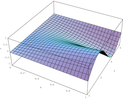
At this point, we can plot the table of data in Cartesian coordinates by using ListPlot3D, with r on on the x-axis, θ on the y-axis and f(r,θ) on the z-axis. This gives an ordinary SurfaceGraphics output.
gr1 = ListPlot3D[
    data,                                (*The array of height values*)
    DataRange -> {{0, rmax}, {0, 2*Pi}}];(*The range that this array covers*)
The image below shows the SurfaceGraphics output, gr1. Note that in this example, the image has been antialiased. Please see the image page for the antialisaing code.

We now convert the SurfaceGraphics object to a Graphics3D object, gr2,:
gr2 = Graphics3D[gr1];
This is the point at which we transform our Cartesian plot into a polar plot using the relations above. We first define a rule to perform the transformation on a point given by a list of three numbers in the form {x,y,z}. We shall call it "substitution":
substitution = {r_, theta_, z_} -> {r Cos[theta], r Sin[theta], z};
Now, we use the ReplaceAll function to go through the Graphics3D object, gr2, and find every polygon point. We set polygon points (a list of three numbers) to be a pattern object using the ":" operator and assign it the name "p". Now we use RuleDelayed (:>) to perform the transformation above on each point. We cannot use Rule (->) as that would only evaluate when it was entered, not when it was used, and would not transaform the points.
gr3 = ReplaceAll[gr2, p : Polygon[pts_] :> ReplaceAll[p,substitution] ]
The last step is to show the resulting polar plot, gr3:
Show[
  gr3,
  AxesLabel -> {"", "", z}]             (*Retitle the axes*)
As we are no longer working in the Cartesian coordinate system, we cannot name the horizontal axes x and y, however, we did not alter the value of z so we can leave that as the name of the vertical axis.

For Mathematica 6.0, please use the next code:
MyListPolarPlot3D[data_, rRange_, thetaRange_, zRange_] :=
 Module[
  {},
  gr1 = ListPlot3D[
    data,
    DataRange -> {
      { rRange[[1]], rRange[[2]]},
      { thetaRange[[1]], thetaRange[[2]]}
      },
    DisplayFunction -> Identity,
    ColorFunction -> "SolarColors",
    ColorFunction -> Automatic,
    MeshFunctions -> {Function[{x, y, z}, x*Cos[y]],
      Function[{x, y, z}, x*Sin[y]]},
    BoundaryStyle -> None,
    ColorFunctionScaling -> True,
    Mesh -> 30
    ];

  substitution = {r_, theta_, z_} -> {r Cos[theta], r Sin[theta], z};

  gr2 = gr1 /.
    GraphicsComplex[p_List, rest__] :>
     GraphicsComplex[ReplaceAll[p, substitution], rest] ;

  (*
  * Retitle the axes and show final graph
  *)
  Return[
   Show[
    gr2,
    AxesLabel -> {"X", "Y", "Z"},
    DisplayFunction -> $DisplayFunction ,
    BoxRatios -> {1, 1, 0.8},
    PlotRange -> {
      {-0.65*rRange[[2]], 0.65*rRange[[2]]},
      {-0.65 rRange[[2]], 0.65*rRange[[2]]},
      {zRange[[1]], zRange[[2]]}
      }
    ]
   ] ;
  ]
This is an example
Fun[r_, t_] :=
  0.632 (0.710 \[ExponentialE]^(-1.166 (0.492+ r^2 -
         1.403 r Cos[t])) +
     0.710 \[ExponentialE]^(-1.166 (0.492+ r^2 + 1.403 r Cos[t]))) ;

dataPlot =
  Table[ Fun[r, t], {t, 0.0, 2.0*Pi, 2*Pi/100}, {r, 0.0, 4.0,
    0.08}] ;
MyListPolarPlot3D[ dataPlot, {0.0, 4.0}, {0.0, 2*Pi}, {0, 0.55}]


