Control Systems/Open source tools/Scilab

Scilab is an open source, cross-platform numerical computational package and a high-level, numerically oriented programming language. It is similar in its capabilities to MATLAB.

Scilab has a good implementation of many of the required control systems functions and has a dynamic model simulator called XCos that makes it a good tool for use by control engineers.

This article will outline the Scilab methods needed to implement the functions described in the main section of this wikibook.

Classical Control Methods

Transfer Functions

Consider the following 2nd order transfer function:

$G(s)={\frac {5s+10}{s^{2}+4s+5}}$

This is created in the Scilab console by the following:

s = poly(0,'s');                                  // Define the complex number frequency parameter. Alternatively you can use s = %s.
TF = syslin("c", (5*s + 10) / (s^2 +4*s +5))      // Define the linear continuous transfer function
TF  =

    10 + 5s     
   ---------    
             2  
   5 + 4s + s   

This transfer function will be used in subsequent demonstrations on this page.

Converting Transfer Functions to/from State Space

Scilab has a functions to perform the necessary conversions.

Conversion to state space is achieved via:

SS = tf2ss(TF)                    // TF -> SS
SS  =
      SS(1)   (state-space system:)
!lss  A  B  C  D  X0  dt  !

      SS(2) = A matrix = 
 - 2.25  - 0.25  
   4.25  - 1.75  

      SS(3) = B matrix = 
 - 2.7386128  
   2.7386128  

      SS(4) = C matrix = 
 - 1.8257419    1.110D-16  

      SS(5) = D matrix = 
   0.  

      SS(6) = X0 (initial state) = 
   0.  
   0.  

      SS(7) = Time domain = 
c

And to convert back to transfer functions you can use:

TFx = clean(ss2tf(SS))            // SS -> TF conversion. Clean removes rounding errors and is recommended.
TFx  =

    10 + 5s     
   ---------    
             2  
   5 + 4s + s

System Representation

Step Response

Step responses are a standard way to represent a dynamic system and to visualize the function. If we subject the example transfer function to a unit step test we get:

Which is produced using the following Scilab code;

t=0:0.01:3;                         // Define a time range for the step test
plot2d(t, csim('step',t,TF));       // csim applies the step test and plot2d produces the graphical output
xlabel("Time [s]");                 // Add a title and label axis
ylabel("y1");
title("Step Response");
xgrid(1, 1, 10);                    // Define a nice grid for the plot to make it easier to read

'csim' performs a general purpose continuous simulation function and can be used in various ways.

The first parameter in the csim function is the simulation function to apply to the transfer function. The options for this parameter can be;

• step
• impulse
• a function : [inputs]=u(t)
• a list : list(ut,parameter1,....,parametern) such that: inputs=ut(t,parameter1,....,parametern) (ut is a function)
• a vector giving the values of u corresponding to each t value

The third parameter ("TF" in the example) is the SIMO linear system to apply the simulation too. State space representations can be used in place of Laplace representation.

A discrete time simulation function is also available called 'dsimul' which can be applied to state space equations.

Bode Plots

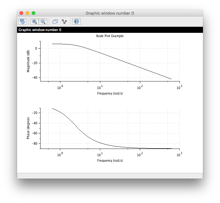
There is an inbuilt command to generate Bode plots such as this example;

To generate the above use the following Scilab code:

clf();                              // Clears the plotting window
f = 0.1:100;                        // Set-up the frequency range we want
bode(TF, f);                        // Generate the Bode plot
title("Bode Plot Example");         // Add a title

Stability

Nyquist Plot

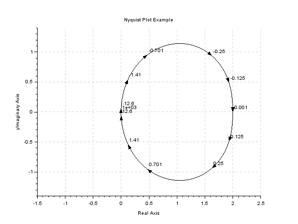
There is an inbuilt command to generate Nyquist plots such as this example;

To generate the above use the following Scilab code:

clf();                              // Clears the plotting window
nyquist(TF);                        // Generate the Bode plot
title("Nyquist Plot Example");      // Add a title and label axis
xlabel("Real Axis");                
ylabel("yImaginary Axis");

The transfer function passed to the nyquist command can be a continuous or a discrete time SIMO linear dynamical system.

Nyquist plots are needed to analyse the Stability Criteria.

Further reading

• Scilab official site
• Scilab Ninja's Control Engineering Basics A resource demonstrating the use of Scilab in control systems work.

Control Systems