Communication Systems/Print Version
| This is the print version of Communication Systems You won't see this message or any elements not part of the book's content when you print or preview this page. |
Current Status:
Introduction[edit | edit source]
This book will eventually cover a large number of topics in the field of electrical communications. The reader will also require a knowledge of Time and Frequency Domain representations, which is covered in-depth in the Signals and Systems book. This book will, by necessity, touch on a number of different areas of study, and as such is more than just a text for aspiring Electrical Engineers. This book will discuss topics of analog communication schemes, computer programming, network architectures, information infrastructures, communications circuit analysis, and many other topics. It is a large book, and varied, but it should be useful to any person interested in learning about an existing communication scheme, or in building their own. Where previous Electrical Engineering books were grounded in theory (notably the Signals and Systems book), this book will contain a lot of information on current standards, and actual implementations. It will discuss how current networks and current transmission schemes work, and may even include information for the intrepid engineer to create their own versions of each.
This book is still in an early stage of development. Many topics do not yet have pages, and many of the current pages are stubs. Any help would be greatly appreciated.
Table of Contents[edit | edit source]
Introduction[edit | edit source]
People are prone to take for granted the fact that modern technology allows us to transmit data at nearly the speed of light to locations that are very far away. 200 years ago, it would be deemed preposterous to think that we could transmit webpages from China to Mexico in less than a second. It would seem equally preposterous to think that people with cellphones could be talking to each other, clear as day, from miles away. Today, these things are so common, that we accept them without even asking how these miracles are possible.
What is Communications?[edit | edit source]
Communications is the field of study concerned with the transmission of information through various means. It can also be defined as technology employed in transmitting messages. It can also be defined as the inter-transmitting the content of data (speech, signals, pulses etc.) from one node to another.
To Whom is This Book For?[edit | edit source]
This book is for people who have read the Signals and Systems wikibook, or an equivalent source of the information. Topics considered in this book will rely heavily on knowledge of Fourier Domain representation and the Fourier Transform. This book can be used to accompany a number of different classes spanning the 3rd and fourth years in a study of electrical engineering. Knowledge of integral and differential calculus is assumed. The reader may benefit from knowledge of such topics as semiconductors, electromagnetic wave propagation, etc., although these topics are not necessary to read and understand the information in this book.
What will this Book Cover[edit | edit source]
This book is going to take a look at nearly all facets of electrical communications, from the shape of the electrical signals, to the issues behind massive networks. It makes little sense to be discussing these subjects outside the realm of current examples. We have the Internet, so in discussing issues concerning digital networks, it makes good sense to reference these issues to the Internet. Likewise, this book will attempt to touch on, at least briefly, every major electrical communications network that people deal with on a daily basis. From AM radio to the Internet, from DSL to cable TV, this book will attempt to show how the concepts discussed apply to the real world.
This book also acknowledges a simple point: It is easier to discuss the signals and the networks simultaneously. For this kind of task to be undertaken in a paper book would require hundreds, if not thousands of printed pages, but through the miracle of Wikimedia, all this information can be brought together in a single, convenient location.
This book would like to actively solicit help from anybody who has experience with any of these concepts: Computer Engineers, Communications Engineers, Computer Programmers, Network Administrators, IT Professionals. Also, this book may cover all these topics, but the reader doesn't need to have prior knowledge of all these disciplines to advance. Information will be developed as completely as possible in the text, and links to other information sources will be provided as needed.
Where to Go From Here[edit | edit source]
Since this book is designed for a junior and senior year of study, there aren't necessarily many topics that will logically follow this book. After reading and understanding this material, the next logical step for the interested engineer is either industry or graduate school. Once in graduate school, there are a number of different areas to concentrate study in. In industry, the number is even higher.
Division of Material[edit | edit source]
Admittedly, this is a very large topic, one that can span not only multiple printed books, but also multiple bookshelves. It could then be asked "Why don't we split this book into 2 or more smaller books?" This seems like a good idea on the surface, but you have to consider exactly where the division would take place. Some would say that we could easily divide the information between "Analog and Digital" lines, or we could divide up into "Signals and Systems" books, or we could even split up into "Transmissions and Networks" Books. But in all these possible divisions, we are settling for having related information in more than 1 place.
Analog and Digital[edit | edit source]
It seems most logical that we divide this material along the lines of analog information and digital information. After all, this is a "digital world", and aspiring communications engineers should be able to weed out the old information quickly and easily. However, what many people don't realize is that digital methods are simply a subset of analog methods with more stringent requirements. Digital transmissions are done using techniques perfected in analog radio and TV broadcasts. Digital computer modems are sending information over the old analog phone networks. Digital transmissions are analyzed using analog mathematical concepts such as modulation, SNR (signal to noise ratio), Bandwidth, Frequency Domain, etc... For these reasons, we can simplify both discussions by keeping them in the same book.
Signals and Systems[edit | edit source]
Perhaps we should divide the book in terms of the signals that are being sent, and the systems that are physically doing the sending. This makes some sense, except that it is impossible to design an appropriate signal without understanding the restrictions of the underlying network that it will be sent on. Also, once we develop a signal, we need to develop transmitters and receivers to send them, and those are physical systems as well.
Systems Approach[edit | edit source]
It is a bit confusing to be writing a book about Communication Systems and also considering the pedagogical Systems Approach. Although using the same word, they are not quite the same thing.
This approach is almost identical to the description above (Signals & Systems) except that it is not limited to the consideration of signals (common in many university texts), but can include other technological drivers (codecs, lasers, and other components).
In this case we give a brief overview of different communication systems (voice, data, cellular, satellite etc.) so that students will have a context in which to place the more detailed (and often generic) information. Then we can then zoom in on the mathematical and technological details to see how these systems do their magic. This lends itself quite well to technical subjects since the basic systems (or mathematics) change relatively slowly, but the underlying technology can often change rapidly and take unexpected terns.
I would like to suggest that the table of contents in this book be rearranged to reflect this pedagogical approach: Systems examples first, followed by the details.
Why would anyone want to study (tele)communications?[edit | edit source]
Telecommunications is an alluring industry with a provocative history filled with eccentric personalities: Bell, Heavyside, Kelvin, Brunel and many others. It is fraught with adventure and danger: adventure spanning space and time; danger ranging from the remote depths of the ocean floor to deep space, from the boardrooms of AT&T to the Hong Kong stock exchange.
Telecommunications has been heralded as a modern Messiah and cursed as a pathetic sham. It has created and destroyed empires and institutions. It has proclaimed the global village while sponsoring destructive nationalism. It has come to ordinary people, but has remained largely in the control of the ‘media’ and even 'big brother'. Experts will soon have us all traveling down a techno-information highway, destination — unknown.
Telecommunications has become the lifeblood of modern civilization. Besides all that, there’s big bucks in it
About This Book[edit | edit source]
There are a few points about this book that are worth mentioning:
Real-world examples will appear in these boxes. |
- The programming parts of this book will not use any particular language, although we may consider particular languages in dedicated chapters.
This page will attempt to show some of the basic history of electrical communication systems.
Chronology[edit | edit source]
1831 Samuel Morse invents the first repeater and the telegraph is born
1837 Charles Wheatstone patents "electric telegraph"
1849 England to France telegraph cable goes into service—and fails after 8 days.
1850 Morse patents "clicking" telegraph.
1851 England-France commercial telegraph service begins. This one uses gutta-percha, and survives.
1858 August 18 - First transatlantic telegraph messages sent by the Atlantic Telegraph Co. The cable deteriorated quickly, and failed after 3 weeks.
1861 The first transcontinental telegraph line is completed
1865 The first trans-Atlantic cable goes in service
1868 First commercially successful transatlantic telegraph cable completed between UK and Canada, with land extension to USA. The message rate is 2 words per minute.
1870 The trans-Atlantic message rate is increased to 20 words per minute.
1874 Baudot invents a practical Time Division Multiplexing scheme for telegraph. Uses 5-bit codes & 6 time slots—90 bps max. rate. Both Western Union and Murray would use this as the basis of multiplex telegraph systems.
1875 Typewriter invented.
1876 Alexander Graham Bell and Elisa Grey independently invent the telephone (although it may have been invented by Antonio Meucci as early as 1857)
1877 Bell attempts to use telephone over the Atlantic telegraph cable. The attempt fails.
1880 Oliver Heaviside's analysis shows that a uniform addition of inductance into a cable would produce distortionless transmission.
1883 Test calls placed over five miles of under-water cable.
1884 - San Francisco-Oakland gutta-percha cable begins telephone service.
1885 Alexander Graham Bell incorporated AT&T
1885 James Clerk Maxwell predicts the existence of radio waves
1887 Heinrich Hertz verifies the existence of radio waves
1889 Almon Brown Strowger invents the first automated telephone switch
1895 Gugliemo Marconi invents the first radio transmitter/receiver
1901 Gugliemo Marconi transmits the first radio signal across the Atlantic 1901 Donald Murray links typewriter to high-speed multiplex system, later used by Western Union
1905 The first audio broadcast is made
1910 Cheasapeake Bay cable is first to use loading coils underwater
1911 The first broadcast license is issued in the US
1912 Hundreds on the Titanic were saved due to wireless
1915 USA transcontinental telephone service begins (NY-San Francisco).
1924 The first video signal is broadcast
1927 First commercial transatlantic radiotelephone service begins
1929 The CRT display tube is invented
1935 Edwin Armstrong invents FM
1939 The Blitzkrieg and WW II are made possible by wireless
1946 The first mobile radio system goes into service in St. Louis
1948 The transistor is invented
1950 Repeatered submarine cable used on Key West-Havana route.
1956 The first trans-Atlantic telephone cable, TAT-1, goes into operation. It uses 1608 vacuum tubes.
1957 The first artificial satellite, Sputnik goes into orbit
1968 The Carterphone decision allows private devices to be attached to the telephone
1984 The MFJ (Modification of Final Judgement) takes effect and the Bell system is broken up
1986 The first transAtlantic fiber optic cable goes into service
Claude Shannon[edit | edit source]
Harry Nyquist[edit | edit source]
Communications Basics[edit | edit source]
It is important to know the difference between a baseband signal, and a broad band signal. In the Fourier Domain, a baseband signal is a signal that occupies the frequency range from 0 Hz up to a certain cutoff. It is called the baseband because it occupies the base, or the lowest range of the spectrum.
In contrast, a broadband signal is a signal which does not occupy the lowest range, but instead a higher range, 1 MHz to 3 MHz, for example. A wire may have only one baseband signal, but it may hold any number of broadband signals, because they can occur anywhere in the spectrum.
Wideband vs Narrowband[edit | edit source]
in form of frequency modulation. wideband fm has been defined as that in which the modulation index normally exceeds unity.
Frequency Spectrum[edit | edit source]
A graphical representation of the various frequency components on a given transmission medium is called a frequency spectrum.
Consider a situation where there are multiple signals which would all like to use the same wire (or medium). For instance, a telephone company wants multiple signals on the same wire at the same time. It certainly would save a great deal of space and money by doing this, not to mention time by not having to install new wires. How would they be able to do this? One simple answer is known as Time-Division Multiplexing.
Time Division Multiplexing[edit | edit source]
Time-Division Multiplexing (TDM) is a convenient method for combining various digital signals onto a single transmission media such as wires, fiber optics or even radio. These signals may be interleaved at the bit, byte, or some other level. The resulting pattern may be transmitted directly, as in digital carrier systems, or passed through a modem to allow the data to pass over an analog network. Digital data is generally organized into frames for transmission and individual users assigned a time slot, during which frames may be sent. If a user requires a higher data rate than that provided by a single channel, multiple time slots can be assigned.
Digital transmission schemes in North America and Europe have developed along two slightly different paths, leading to considerable incompatibility between the networks found on the two continents.
BRA (basic rate access) is a single digitized voice channel, the basic unit of digital multiplexing.

North American TDM[edit | edit source]
The various transmission rates are not integral numbers of the basic rate. This is because additional framing and synchronization bits are required at every multiplexing level.

In North America, the basic digital channel format is known as DS-0. These are grouped into frames of 24 channels each. A concatenation of 24 channels and a start bit is called a frame. Groups of 12 frames are called multiframes or superframes. These vary the start bit to aid in synchronizing the link and add signaling bits to pass control messages.

S Bit Synchronization[edit | edit source]
The S bit is used to identify the start of a DS-1 frame. There are 8 thousand S bits per second. They have an encoded pattern, to aid in locating channel position within the frame.

This forms a regular pattern of 1 0 1 0 1 0 for the odd frames and 0 0 1 1 1 0 for the even frames. Additional synchronization information is encoded in the DS-1 frame when it is used for digital data applications, so lock is more readily acquired and maintained.
For data customers, channel 24 is reserved as a special sync byte, and bit 8 of the other channels is used to indicate if the remaining 7 bits are user data or system control information. Under such conditions, the customer has an effective channel capacity of 56 Kbps.
To meet the needs of low speed customers, an additional bit is robbed to support sub-rate multiplexer synchronization, leaving 6 x 8 Kbps = 48 Kbps available. Each DS-0 can be utilized as:
- • 5 x 9.6 Kbps channels or
- • 10 x 4.8 Kbps channels or
- • 20 x 2.48 Kbps channels.
In the DS-2 format, 4 DS-1 links are interleaved, 12 bits at a time. An additional 136 Kbps is added for framing and control functions resulting in a total bit rate of 6.312 Mbps.
Signaling[edit | edit source]
Signaling provides control and routing information. Two bits, called the A and B bits, are taken from each channel in frames 6 and 12 in the multiframe. The A bit is the least significant bit in each channel in frame 6, and the B bit is the least significant bit in each channel in frame 12. This provides a signaling rate of 666 2/3 bps per channel.
The quality of voice transmission is not noticeably affected when 2% of the signal is robbed for signaling. For data, it may be a different story. If the data is encoded in an analog format such as FSK or PSK, then robbing bits is of no consequence, but if the data is already in digital form, then robbing bits results in unacceptable error rates. It is for this reason that in North America, a 64 Kbps clear channel cannot readily be switched through the PSTN. This means that data customers are limited to 56 Kbps clear channels. This simple condition has a profound effect on the development of new services such as ISDN. In most facilities, the A and B bits represent the status of the telephone hook switch, and correspond to the M lead on the E&M interface of the calling party.
ESF[edit | edit source]
CCITT has modified the North American digital hierarchy for the deployment of ISDN, by means of recommendation G.704. ESF consists of 24 DS-0 channels in a frame, but groups them into a 24-frame multiframe instead of the usual 12-frame multiframe.
The S bit is renamed the F bit, but only 1/4 of them are used for synchronization. This is possible because of improvements in frame search techniques and allows more signaling states to be defined.
Bit robbing is still used for signaling over an ESF link, but with the advent of ISDN, it will not be permitted. Instead, channel 24 is used to support a D channel.

Typical T1 CPE Application[edit | edit source]
The large telecom carriers are not the only ones who deploy high-speed TDM facilities. In many cases, heavy users of voice or data services can reduce their transmission costs by concentrating their numerous low speed lines on to a high speed facility.
There are many types of T1 multiplexers available today. Some are relatively simple devices, while others allow for channel concatenation, thus supporting a wide range of data rates. The ability to support multiple DS-0s allows for easy facilitation of such protocols as the video teleconferencing standard, Px64.

Multiplexers[edit | edit source]
Multiplexing units are often designated by the generic term Mab where a is input DS level and b is the output DS level. Thus, an M13 multiplexer combines 28 DS–1s into a single DS–3 and an M23 multiplexer combines 7 DS–2s into a single DS–3.

ZBTSI[edit | edit source]
ZBTSI (zero byte time slot interchange) is used on DS–4 links. Four DS-1 frames are loaded into a register, and renumbered 1–96. If there are any empty slots [all zeros], the first framing bit is inverted and all blank slots are relocated to the front of the frame. Channel 1 is then loaded with a 7-bit number corresponding to the original position of the first empty slot. Bit 8 used to indicate whether the following channel contains user information or another address for an empty slot.
If there is a second vacancy, bit 8 in the previous channel is set, and the empty slot address is placed in channel 2. This process continues until all empty positions are filled.
The decoding process at the receiver is done in reverse. Borrowing 1 in 4 framing bits for this system is not enough to cause loss of synchronization and provides a 64 Kbps clear channel to the end-user.
European TDM Carriers[edit | edit source]
European systems were developed along slightly different principles. The 64 Kbps channel is still the basic unit, but signaling is not included in each channel. Instead, common channel signaling is used. In a level 1 carrier, channels 0 and 16 are reserved for signaling and control. This subtle difference means that European systems did not experience the toll fraud and 56 k bottlenecks common to North American systems, and they experience a much larger penetration of ISDN services.


Zero Substitutions[edit | edit source]
In order to prevent transmission systems from loosing lock on the data stream, it is necessary to avoid long strings of zeros. One of the most effective ways of doing this is to replace the zeros with a predetermined code. This substitution must be done in such a way that the receiver can identify it and strip it off before passing the data stream to the client.
AMI provides a simple means of detecting substitutions. In the normal course of events, alternate marks are inverted. Therefor, deliberately inducing a bipolarvariation at the transmitter can alert the receiver of a substitution. However, a single violation is indistinguishable from a transmission error. Consequently, some additional condition must also occur.
There are two common methods to create a second condition:
- · Create a second bipolar violation in the opposite direction, within a specified time. This has the effect of keeping the average signal level at zero.
- · Count the number of marks from the last substitution to predict the next type of violation
B6ZS[edit | edit source]
B6ZS (binary six zero substitution) is used on T2 AMI transmission links.
Synchronization can be maintained by replacing strings of zeros with bipolar violations. Since alternate marks have alternate polarity, two consecutive pulses of the same polarity constitute a violation. Therefore, violations can be substituted for strings of zeros, and the receiver can determine where substitutions were made.
Since the last mark may have been either positive (+) or negative (-), there are two types of substitutions:

These substitutions force two consecutive violations. A single bit error does not create this condition.

B8ZS[edit | edit source]
This scheme uses the same substitution as B6ZS.

B3ZS[edit | edit source]
B3ZS is more involved than B6ZS, and is used on DS–3 carrier systems. The substitution is not only dependent on the polarity of the last mark, but also on the number of marks since the last substitution.


HDB3[edit | edit source]
HDB3 (high density binary 3) introduces bipolar violations when four consecutive zeros occur. It can therefore also be called B4ZS. The second and thirds zeros are left unchanged, but the fourth zero is given the same polarity as the last mark. The first zero may be modified to a one to make sure that successive violations are of alternate polarity.

HDB3 is used in Europe. Violation, or V pulses are injected after three consecutive zeros. The fourth zero is given the same polarity as the last mark. In the event of long strings of zeros occurring, a succession of single polarity pulses would occur, and a dc offset would build-up.
To prevent this, the first zero in a group of 4, may be modified to a 1. This B or balancing pulse assures that successive violations are of alternate polarity.

Block Code Substitution[edit | edit source]
These schemes operate on bytes rather than a bit at a time. Some transmit the signal as binary levels, but most use multi-level pulses. Some authors categorize these as line codes.
A binary block code has the designation nBmB, where n input bits are encoded into m output bits. The most common of these is the 3B4B code.

In Europe 4B3T, which encodes 4 binary bits into 3 ternary levels, has been selected as the BRA for ISDN. In North America, 2B1Q which encodes 2 binary bits into 1 quaternary level has been selected for BRA.

Some block codes do not generate multilevel pulses. For example, 24B1P or 24B25B simply adds a P or parity bit to a 24 bit block.
Benefits of TDM[edit | edit source]
TDM is all about cost: fewer wires and simpler receivers are used to transmit data from multiple sources to multiple destinations. TDM also uses less bandwidth than Frequency-Division Multiplexing (FDM) signals, unless the bitrate is increased, which will subsequently increase the necessary bandwidth of the transmission.
Synchronous TDM[edit | edit source]
Synchronous TDM is a system where the transmitter and the receiver both know exactly which signal is being sent. Consider the following diagram:
Signal A ---> |---| |A|B|C|A|B|C|   |------| ---> Signal A
Signal B ---> |TDM| --------------> |De-TDM| ---> Signal B
Signal C ---> |---|                 |------| ---> Signal C
In this system, starting at time-slice 0, every third time-slice is reserved for Signal A; starting at time-slice 1, every third time-slice is reserved for Signal B; and starting at time-slice 2, every third time-slice is reserved for Signal C. In this situation, the receiver (De-TDM) needs only to switch after the signal on each time-slice is received.
The data flow of each input connection is divided into units where each input occupies one input time slot. Each input connection has a time slot alloted in the output irrespective of the fact whether it is sending data or not.
      A -----|A3|A2|A1|---> |---| .............|C3|B3|A3|C2|B2|A2|C1|B1|A1|   |------| --->  A
             |  |  |  |                        |        |        |
      B -----|B3|B2|B1|---> |MUX| -------------|--------|--------|----------> |De-MUX| --->  B
             |  |  |  |                        |        |        |
      C -----|C3|C2|C1|---> |---|              |        |        |            |------| --->  C
                   <-->                                 <-------->
                  Bit Interval                       Frame (x seconds)
Sync TDM is inefficient when one or more input lines have no data to send. Thus, it is used with lines with high data traffic.
Sampling rate is same for all signals. Maximum sampling rate = twice the maximum frequency all the signals.
Statistical TDM[edit | edit source]
Synchronous TDM is beneficial because the receiver and transmitter can both cost very little. However, consider the most well-known network: the Internet. In the Internet, a given computer might have a data rate of 1kbps when hardly anything is happening, but might have a data rate of 100kbps when downloading a large file from a fast server. How are the time-slices divided in this instance? If every time slice is made big enough to hold 100Kbps, when the computer isn't downloading any data, all of that time and electricity will be wasted. If every time-slice is only big enough for the minimum case, the time required to download bigger files will be greatly increased.
The solution to this problem is called Statistical TDM, and is the solution that the Internet currently uses. In Statistical TDM, each data item, known as the payload (we used time-slices to describe these earlier), is appended with a certain amount of information about who sent it, and who is supposed to receive it (the header). The combination of a payload and a header is called a packet. Packets are like envelopes in the traditional "snail mail" system: Each packet contains a destination address and a return address as well as some enclosed data. Because of this, we know where each packet was sent from and where it is going.
The downside to statistical TDM is that the sender needs to be smart enough to write a header, and the receiver needs to be smart enough to read the header and (if the packet is to be forwarded,) send the packet toward its destination.
Link Utilization[edit | edit source]
Statistical multiplexing attempts to maximize the use of a communication path. The study of this is often called queuing theory. A queue is simply a line of customers or packets waiting to be served. Under most circumstances, the arrival rate is unpredictable and therefor follows a random or Poisson distribution pattern, whereas the service time is constant.
The utilization or fraction of time actually used by a packet multiplexing system to process packets is given by:

The queue length or average number of items waiting to be served is given by:


- Example
- A T1 link has been divided into a number of 9.6 Kbps channels and has a combined user data rate of 1.152 Mbps. Access to this channel is offered to 100 customers, each requiring 9.6 Kbps data 20% of the time. If the user arrival time is strictly random find the T1 link utilization.
- Solution
- The utilization or fraction of time used by the system to process packets is given by:

- A 24 channel system dedicated to DATA, can place five 9.6 Kbps customers in each of 23 channels, for a total of 115 customers. In the above statistical link, 100 customers created an average utilization of 0.167 and were easily fitted, with room to spare if they transmit on the average 20% of the time. If however, the customer usage were not randomly distributed, then the above analysis would have to be modified.
This example shows the potential for statistical multiplexing. If channels were assigned on a demand basis (only when the customer had something to send), a single T1 may be able to support hundreds of low volume users.
A utilization above 0.8 is undesirable in a statistical system, since the slightest variation in customer requests for service would lead to buffer overflow. Service providers carefully monitor delay and utilization and assign customers to maximize utilization and minimize cost.
Packets[edit | edit source]
Packets will be discussed in greater detail once we start talking about digital networks (specifically the Internet). Packet headers not only contain address information, but may also include a number of different fields that will display information about the packet. Many headers contain error-checking information (checksum, Cyclic Redundancy Check) that enables the receiver to check if the packet has had any errors due to interference, such as electrical noise.
Duty Cycles[edit | edit source]
Duty cycle is defined as " the time that is effectively used to send or receive the data, expressed as a percentage of total period of time." The more the duty cycle , the more effective transmission or reception.
We can define the pulse width, τ, as being the time that a bit occupies from within its total alloted bit-time Tb. If we have a duty cycle of D, we can define the pulse width as:

Where:

The pulse width is equal to the bit time if we are using a 100% duty cycle.
Introduction[edit | edit source]
It turns out that many wires have a much higher bandwidth than is needed for the signals that they are currently carrying. Analog Telephone transmissions, for instance, require only 3 000 Hz of bandwidth to transmit human voice signals. Over short distances, however, twisted-pair telephone wire has an available bandwidth of nearly 100000 Hz!
There are several terrestrial radio based communications systems deployed today. They include:
- Cellular radio
- Mobile radio
- Digital microwave radio
Mobile radio service was first introduced in the St. Louis in 1946. This system was essentially a radio dispatching system with an operator who was able to patch the caller to the PSTN via a switchboard. Later, an improved mobile telephone system, IMTS, allowed customers to dial their own calls without the need for an operator. This in turn developed into the cellular radio networks we see today.
The long haul PSTNs and packet data networks use a wide variety of transmission media including
- Terrestrial microwave
- Satellite microwave
- Fiber optics
- Coaxial cable
In this section, we will be concerned with terrestrial microwave systems. Originally, microwave links used FDM exclusively as the access technique, but recent developments are changing analog systems to digital where TDM is more appropriate.
Fixed Access Assignment[edit | edit source]
Three basic methods can be used to combine customers on to fixed channel radio links:
- FDMA - (Frequency division multiple access) analog or digital
- TDMA - (Time division multiple access) three conversation paths are time division multiplexed in 6.7 mSec time slots on a single carrier.
- CDMA - (Code division multiple access) this uses spread spectrum techniques to increase the subscriber density. The transmitter hops through a pseudo-random sequence of frequencies. The receiver is given the sequence list and is able to follow the transmitter. As more customers are added to the system, the signal to noise will gradually degrade. This is in contrast to AMPS where customers are denied access once all of the frequencies are assigned code division multiple access [digital only]

What is FDM?[edit | edit source]
Frequency Division Multiplexing (FDM) allows engineers to utilize the extra space in each wire to carry more than one signal. By frequency-shifting some signals by a certain amount, engineers can shift the spectrum of that signal up into the unused band on that wire. In this way, multiple signals can be carried on the same wire, without having to divy up time-slices as in Time-Division Multiplexing schemes.In analog transmission, signals are commonly multiplexed using frequency-division multiplexing (FDM), in which the carrier bandwidth is divided into subchannels of different frequency widths, each carrying a signal at the same time in parallel
Broadcast radio and television channels are separated in the frequency spectrum using FDM. Each individual channel occupies a finite frequency range, typically some multiple of a given base frequency. |
Traditional terrestrial microwave and satellite links employ FDM. Although FDM in telecommunications is being reduced, several systems will continue to use this technique, namely: broadcast & cable TV, and commercial & cellular radio.
Analog Carrier Systems[edit | edit source]
The standard telephony voice band [300 – 3400 Hz] is heterodyned and stacked on high frequency carriers by single sideband amplitude modulation. This is the most bandwidth efficient scheme possible.

The analog voice channels are pre-grouped into threes and heterodyned on carriers at 12, 16, and 20 kHz. The resulting upper sidebands of four such pregroups are then heterodyned on carriers at 84, 96, 108, and 120 kHz to form a 12-channel group.
Since the lower sideband is selected in the second mixing stage, the channel sequence is reversed and a frequency inversion occurs within each channel.

This process can continue until the available bandwidth on the coaxial cable or microwave link is exhausted.

In the North American system, there are:
- 12 channels per group
- 5 groups per supergroup
- 10 super groups per mastergroup
- 6 master groups per jumbogroup
In the European CCITT system, there are:
- 12 channels per group
- 5 groups per supergroup
- 5 super groups per mastergroup
- 3 master groups per supermastergroup
There are other FDM schemes including:
- L600 - 600 voice channels 60–2788 kHz
- U600 - 600 voice channels 564–3084 kHz
- L3 - 1860 voice channels 312–8284 kHz, comprised of 3 mastergroups and a supergroup
- L4 - 3600 voice channels, comprised of six U600s
Benefits of FDM[edit | edit source]
FDM allows engineers to transmit multiple data streams simultaneously over the same channel, at the expense of bandwidth. To that extent, FDM provides a trade-off: faster data for less bandwidth. Also, to demultiplex an FDM signal requires a series of bandpass filters to isolate each individual signal. Bandpass filters are relatively complicated and expensive, therefore the receivers in an FDM system are generally expensive.
Examples of FDM[edit | edit source]
As an example of an FDM system, Commercial broadcast radio (AM and FM radio) simultaneously transmits multiple signals or "stations" over the airwaves. These stations each get their own frequency band to use, and a radio can be tuned to receive each different station. Another good example is cable television, which simultaneously transmits every channel, and the TV "tunes in" to which channel it wants to watch.
Orthogonal FDM[edit | edit source]
Orthogonal Frequency Division Multiplexing (OFDM) is a more modern variant of FDM that uses orthogonal sub-carriers to transmit data that does not overlap in the frequency spectrum and is able to be separated out using frequency methods. OFDM has a similar data rate to traditional FDM systems, but has a higher resilience to disruptive channel conditions such as noise and channel fading.
Voltage Controlled Oscillators (VCO)[edit | edit source]
A voltage-controlled oscillator (VCO) is a device that outputs a sinusoid of a frequency that is a function of the input voltage. VCOs are not time-invariant, linear components. A complete study of how a VCO works will have to be relegated to a more detailed section based on feedback and oscillators. This page will, however, attempt to answer some of the basic questions about VCOs.
A basic VCO has input/output characteristics as such:
v(t) ----|VCO|----> sin(a[f + v(t)]t + O)
VCOs are often implemented using a special type of diode called a "Varactor". Varactors, when reverse-biased, produce a small amount of capacitance that varies with the input voltage.
Phase-Locked Loops[edit | edit source]
If you are talking on your cellphone, and you are walking (or driving), the phase angle of your signal is going to change, as a function of your motion, at the receiver. This is a fact of nature, and is unavoidable. The solution to this then, is to create a device which can "find" a signal of a particular frequency, negate any phase changes in the signal, and output the clean wave, phase-change free. This device is called a Phase-Locked Loop (PLL), and can be implemented using a VCO.
Purpose of VCO and PLL[edit | edit source]
VCO and PLL circuits are highly useful in modulating and demodulating systems. We will discuss the specifics of how VCO and PLL circuits are used in this manner in future chapters.
Varactors[edit | edit source]
As a matter of purely professional interest, we will discuss varactors here.
Further reading[edit | edit source]
- Clock and data recovery has detailed information about designing and analyzing PLLs. (VCO)
What is an Envelope Filter?[edit | edit source]
The envelope detector is a simple analog circuit that can be used to find the peaks in a quickly-changing waveform. Envelope detectors are used in a variety of devices, specifically because passing a sinusoid through an envelope detector will suppress the sinusoid.
Circuit Diagram[edit | edit source]
In essence, an envelope filter has the following diagram:
o------+------+------o
+      |      |      +
       \     (c)
vin    /R     |     vout
       \      |
-      |      |      -
o------+------+------o
Where (c) represents a capacitor, and R is a resistor. Under zero input voltage (vin = 0), the capacitor carries no charge, and the resistor carries no current. When vin is increased, the capacitor stores charge until it reaches capacity, and then the capacitor becomes an open circuit. At this point, all current in the circuit is flowing through the resistor, R. As voltage decreases, the capacitor begins to discharge it's stored energy, slowing down the state change in the circuit from high voltage to low voltage.
Positive Voltages[edit | edit source]
By inserting a diode at the beginning of this circuit, we can negate the effect of a sinusoid, dipping into negative voltage, and forcing the capacitor to discharge faster:
  diode
o-->|--+------+------o
+      |      |      +
       \     (c)
vin    /R     |     vout
       \      |
-      |      |      -
o------+------+------o
Purpose of Envelope Filters[edit | edit source]
Envelope filters help to find the outer bound of a signal that is changing in amplitude.
Envelope Filters are generally used with AM demodulation, discussed later. |
(Envelope Detectors)
Modulation is a term that is going to be used very frequently in this book. So much in fact, that we could almost have renamed this book "Principles of Modulation", without having to delete too many chapters. So, the logical question arises: What exactly is modulation?
Definition[edit | edit source]
Modulation is a process of mixing a signal with a sinusoid to produce a new signal. This new signal, conceivably, will have certain benefits over an un-modulated signal. Mixing of low frequency signal with high frequency carrier signal is called modulation.

we can see that this sinusoid has 3 parameters that can be altered, to affect the shape of the graph. The first term, A, is called the magnitude, or amplitude of the sinusoid. The next term, is known as the frequency, and the last term, is known as the phase angle. All 3 parameters can be altered to transmit data.


The sinusoidal signal that is used in the modulation is known as the carrier signal, or simply "the carrier". The signal that is used in modulating the carrier signal(or sinusoidal signal) is known as the "data signal" or the "message signal". It is important to notice that a simple sinusoidal carrier contains no information of its own.
In other words we can say that modulation is used because some data signals are not always suitable for direct transmission, but the modulated signal may be more suitable.
Types of Modulation[edit | edit source]
There are 3 basic types of modulation: Amplitude modulation, Frequency modulation, and Phase modulation.
- amplitude modulation
- a type of modulation where the amplitude of the carrier signal is modulated (changed) in proportion to the message signal while the frequency and phase are kept constant.
- frequency modulation
- a type of modulation where the frequency of the carrier signal is modulated (changed) in proportion to the message signal while the amplitude and phase are kept constant.
- phase modulation
- a type of modulation where the phase of the carrier signal is varied accordance to the low frequency of the message signal is known as phase modulation.
Why Use Modulation?[edit | edit source]
Why use modulation at all? To answer this question, let's consider a channel that essentially acts like a bandpass filter: both the lowest frequency components and the highest frequency components are attenuated or unusable in some way, with transmission only being practical over some intermediate frequency range. If we can't send low-frequency signals, then we need to shift our signal up the frequency ladder. Modulation allows us to send a signal over a bandpass frequency range. If every signal gets its own frequency range, then we can transmit multiple signals simultaneously over a single channel, all using different frequency ranges.
Another reason to modulate a signal is to allow the use of a smaller antenna. A baseband (low frequency) signal would need a huge antenna because in order to be efficient, the antenna needs to be about 1/10th the length of the wavelength. Modulation shifts the baseband signal up to a much higher frequency, which has much smaller wavelengths and allows the use of a much smaller antenna.
Examples[edit | edit source]
Think about your car radio. There are more than a dozen (or so) channels on the radio at any time, each with a given frequency: 100.1 MHz, 102.5 MHz etc... Each channel gets a certain range (usually about 0.22 MHz), and the entire bayot gets transmitted over that range. Modulation makes it all possible, because it allows us to send voice and music (which are essential baseband signals) over a bandpass (or "Broadband") channel.
Non-sinusoidal modulation[edit | edit source]
A sine wave at one frequency can be separated from a sine wave at another frequency (or a cosine wave at the same frequency) because the two signals are "orthogonal".
There are other sets of signals, such that every signal in the set is orthogonal to every other signal in the set.
A simple orthogonal set is time multiplexed division (TDM) -- only one transmitter is active at any one time.
Other more complicated sets of orthogonal waveforms—Walsh codes and various pseudo-noise codes such as Gold codes and maximum length sequences—are also used in some communication systems.
The process of combining these waveforms with data signals is sometimes called "modulation", because it is so very similar to the way modulation combines sine waves with data signals.
Further reading[edit | edit source]
- Data Coding Theory/Spectrum Spreading
- Wikipedia:Walsh code
- Wikipedia:Gold code
- Wikipedia:pseudonoise code
- Wikipedia:maximum length sequence
There is lots of talk nowadays about buzzwords such as "Analog" and "Digital". Certainly, engineers who are interested in creating a new communication system should understand the difference. Which is better, analog or digital? What is the difference? What are the pros and cons of each? This chapter will look at the answers to some of these questions.
What are They?[edit | edit source]
What exactly is an analog signal, and what is a digital signal?
- Analog
- Analog signals are continuous in both time and value. Analog signals are used in many systems, although the use of analog signals has declined with the advent of cheap digital signals. All natural signals are Analog in nature or analog signal is that signal which amplitude on Y axis change with time on X axis...
- Digital
- Digital signals are discrete in time and value. Digital signals are signals that are represented by binary numbers, "1" or "0". The 1 and 0 values can correspond to different discrete voltage values, and any signal that doesn't quite fit into the scheme just gets rounded off.
or digital signal is that signal which have certain or fixed value on Y axis change with time on X axis...
Digital signals are sampled, quantized & encoded version of continuous time signals which they represent. In addition, some techniques also make the signal undergo encryption to make the system more tolerant to the channel.
What are the Pros and Cons?[edit | edit source]
Each paradigm has its own benefits and problems
- Analog
- Analog systems are less tolerant to noise, make good use of bandwidth, and are easy to manipulate mathematically. However, analog signals require hardware receivers and transmitters that are designed to perfectly fit the particular transmission.
- Digital
- Digital signals are more tolerant to noise, but digital signals can be completely corrupted in the presence of excess noise. In digital signals, noise could cause a 1 to be interpreted as a 0 and vice versa, which makes the received data different than the original data. Imagine if the army transmitted a position coordinate to a missile digitally, and a single bit was received in error. This single bit error could cause a missile to miss its target by miles. Luckily, there are systems in place to prevent this sort of scenario, such as checksums and CRCs, which tell the receiver when a bit has been corrupted and ask the transmitter to resend the data. The primary benefit of digital signals is that they can be handled by simple, standardized receivers and transmitters, and the signal can be then dealt with in software (which is comparatively cheap to change).
- Discrete Digital and Analogue
Discrete data has a fixed set of possible values.
Digital data is a type of Discrete data where the fixed value can either be 1 or 0.
Analogue data can take on any real value.
Sampling and Reconstruction[edit | edit source]
The process of converting from analog data to digital data is called "sampling". The process of recreating an analog signal from a digital one is called "reconstruction". This book will not talk about either of these subjects in much depth beyond this, although other books on the topic of EE might, such as A-level Physics (Advancing Physics)/Digitisation.
Further reading[edit | edit source]
Signals need a channel to follow, so that they can move from place to place. These Communication Mediums, or "channels" are things like wires and antennae that transmit the signal from one location to another. Some of the most common channels are listed below:
Twisted Pair Wire[edit | edit source]
Twisted Pair is a transmission medium that uses two conductors that are twisted together to form a pair. The concept for the twist of the conductors is to prevent interference. Ideally, each conductor of the pair basically receives the same amount of interference, positive and negative, effectively cancelling the effect of the interference. Typically, most inside cabling has four pairs with each pair having a different twist rate. The different twist rates help to further reduce the chance of crosstalk by making the pairs appear electrically different in reference to each other. If the pairs all had the same twist rate, they would be electrically identical in reference to each other causing crosstalk, which is also referred to as capacitive coupling. Twisted pair wire is commonly used in telephone and data cables with variations of categories and twist rates.
Other variants of Twisted Pair are the Shielded Twisted Pair cables. The shielded types operate very similar to the non-shielded variety, except that Shielded Twisted Pair also has a layer of metal foil or mesh shielding around all the pairs or each individual pair to further shield the pairs from electromagnetic interference. Shielded twisted pair is typically deployed in situations where the cabling is subjected to higher than normal levels of interference.
Coaxial Cable[edit | edit source]
Another common type of wire is Coaxial Cable. Coaxial cable (or simply, "coax") is a type of cable with a single data line, surrounded by various layers of padding and shielding. The most common coax cable, common television cable, has a layer of wire mesh surrounding the padded core, that absorbs a large amount of EM interference, and helps to ensure a relatively clean signal is transmitted and received. Coax cable has a much higher bandwidth than a twisted pair, but coax is also significantly more expensive than an equal length of twisted pair wire. Coax cable frequently has an available bandwidth in excess of hundreds of megahertz (in comparison with the hundreds of kilohertz available on twisted pair wires).
Originally, Coax cable was used as the backbone of the telephone network because a single coaxial cable could hold hundreds of simultaneous phone calls by a method known as "Frequency Division Multiplexing" (discussed in a later chapter). Recently however, Fiber Optic cables have replaced Coaxial Cable as the backbone of the telephone network because Fiber Optic channels can hold many more simultaneous phone conversations (thousands at a time), and are less susceptible to interference, crosstalk, and noise then Coaxial Cable.
Fiber Optics[edit | edit source]
Fiber Optic cables are thin strands of glass that carry pulses of light (frequently infrared light) across long distances. Fiber Optic channels are usually immune to common RF interference, and can transmit incredibly high amounts of data very quickly. There are 2 general types of fiber optic cable: single frequency cable, and multi-frequency cable. single frequency cable carries only a single frequency of laser light, and because of this there is no self-interference on the line. Single-frequency fiber optic cables can attain incredible bandwidths of many gigahertz. Multi-Frequency fiber optics cables allow a Frequency-Division Multiplexed series of signals to each inhabit a given frequency range. However, interference between the different signals can decrease the range over which reliable data can be transmitted.
Wireless Transmission[edit | edit source]
In wireless transmission systems, signals are propagated as Electro-Magnetic waves through free space. Wireless signals are transmitted by a transmitter, and received by a receiver. Wireless systems are inexpensive because no wires need to be installed to transmit the signal, but wireless transmissions are susceptible not only to EM interference, but also to physical interference. A large building in a city, for instance can interfere with cell-phone reception, and a large mountain could block AM radio transmissions. Also, WiFi internet users may have noticed that their wireless internet signals don't travel through walls very well.
There are 2 types of antennas that are used in wireless communications, isotropic, and directional.
Isotropic[edit | edit source]
People should be familiar with isotropic antennas because they are everywhere: in your car, on your radio, etc... Isotropic antennas are omni-directional in the sense that they transmit data out equally (or nearly equally) in all directions. These antennas are excellent for systems (such as FM radio transmission) that need to transmit data to multiple receivers in multiple directions. Also, Isotropic antennas are good for systems in which the direction of the receiver, relative to the transmitter is not known (such as cellular phone systems).
Directional[edit | edit source]
Directional antennas focus their transmission power in a single narrow direction range. Some examples of directional antennas are satellite dishes, and wave-guides. The downfall of the directional antennas is that they need to be pointed directly at the receiver all the time to maintain transmission power. This is useful when the receiver and the transmitter are not moving (such as in communicating with a geo-synchronous satellite).
Receiver Design[edit | edit source]
It turns out that if we know what kind of signal to expect, we can better receive those signals. This should be intuitive, because it is hard to find something if we don't know what precisely we are looking for. How is a receiver supposed to know what is data and what is noise, if it doesnt know what data looks like?
Coherent transmissions are transmissions where the receiver knows what type of data is being sent. Coherency implies a strict timing mechanism, because even a data signal may look like noise if you look at the wrong part of it. In contrast, noncoherent receivers don't know exactly what they are looking for, and therefore noncoherent communication systems need to be far more complex (both in terms of hardware and mathematical models) to operate properly.
This section will talk about coherent receivers, first discussing the "Simple Receiver" case, and then going into theory about what the optimal case is. Once we know mathematically what an optimal receiver should be, we then discuss two actual implementations of the optimal receiver.
It should be noted that the remainder of this book will discuss optimal receivers. After all, why would a communication's engineer use anything that is less than the best?
The Simple Receiver[edit | edit source]
A simple receiver is just that: simple. A general simple receiver will consist of a low-pass filter (to remove excess high-frequency noise), and then a sampler, that will select values at certain points in the wave, and interpolate those values to form a smooth output curve. In place of a sampler (for purely analog systems), a general envelope filter can also be used, especially in AM systems. In other systems, different tricks can be used to demodulate an input signal, and acquire the data. However simple receivers, while cheap, are not the best choice for a receiver. Occasionally they are employed because of their price, but where performance is an issue, a better alternative receiver should be used.
The Optimal Receiver[edit | edit source]
Engineers are able to mathematically predict the structure of the optimal receiver. Read that sentence again: Engineers are able to design, analyze, and build the best possible receiver, for any given signal. This is an important development for several reasons. First, it means that no more research should go into finding a better receiver. The best receiver has already been found, after all. Second, it means any communications system will not be hampered (much) by the receiver.
Derivation[edit | edit source]
here we will attempt to show how the coherent receiver is derived.
Matched Receiver[edit | edit source]
The matched receiver is the logical conclusion of the optimal receiver calculation. The matched receiver convolves the signal with itself, and then tests the output. Here is a diagram:
s(t)----->(Convolve with r(t))----->
This looks simple enough, except that convolution modules are often expensive. An alternative to this approach is to use a correlation receiver.
Correlation Receiver[edit | edit source]
The correlation receiver is similar to the matched receiver, instead with a simple switch: The multiplication happens first, and the integration happens second.
Here is a general diagram:
           r(t)
            |
            v
s(t) ----->(X)----->(Integrator)--->
In a digital system, the integrator would then be followed by a threshold detector, while in an analog receiver, it might be followed by another detector, like an envelope detector.
Conclusion[edit | edit source]
To do the best job of receiving a signal we need to know the form of the signal that we are sending. After all we can't design a receiver until after we've decided how the signal will be sent. This method poses some problems in that the receiver must be able to line up the received signal with the given reference signal to work the magic: if the received signal and the reference signal are out of sync with each other, either as a function of an error in phase or an error in frequency, then the optimal receiver will not work.
Further reading[edit | edit source]
Analog Modulation[edit | edit source]
Analog Modulation Overview[edit | edit source]
Let's take a look at a generalized sinewave:

It consists of three components namely; amplitude, frequency and phase. Each of which can be decomposed to provide finer detail:
![{\displaystyle x(t)=As(t)\sin(2\pi [f_{c}+kf_{m}(t)]t+\alpha \phi (t))}](https://wikimedia.org/api/rest_v1/media/math/render/svg/e26191b10f6cbaafa6b5a021aeb28d221394c62f)
Types of Analog Modulation[edit | edit source]
We can see 3 parameters that can be changed in this sine wave to send information:
- . This term is called the "Amplitude", and changing it is called "Amplitude Modulation" (AM)
- This term is called the "Frequency Shift", and changing it is called "Frequency Modulation"
- . this term is called the "Phase angle", and changing it is called "Phase Modulation".
- The terms frequency and phase modulation are often combined into a more general group called "Angle Modulation".


The Breakdown[edit | edit source]
Each term consists of a coefficient (called a "scaling factor"), and a function of time that corresponds to the information that we want to send. The scaling factor out front, A, is also used as the transmission power coefficient. When a radio station wants their signal to be stronger (regardless of whether it is AM, FM, or PM), they "crank-up" the power of A, and send more power out onto the airwaves.
How we Will Cover the Material[edit | edit source]
We are going to go into separate chapters for each different type of modulation. This book will attempt to discuss some of the mathematical models and techniques used with different modulation techniques. It will also discuss some practical information about how to construct a transmitter/receiver, and how to use each modulation technique effectively.
Amplitude modulation is one of the earliest radio modulation techniques. The receivers used to listen to AM-DSB-C are perhaps the simplest receivers of any radio modulation technique; which may be why that version of amplitude modulation is still widely used today. By the end of this module, you will know the most popular versions of amplitude modulation, some popular AM modulation circuits, and some popular AM demodulation circuits.
Amplitude Modulation[edit | edit source]
Amplitude modulation (AM) occurs when the amplitude of a carrier wave is modulated, to correspond to a source signal. In AM, we have an equation that looks like this:

We can also see that the phase of this wave is irrelevant, and does not change (so we don't even include it in the equation).
AM Radio uses AM modulation |
AM Double-Sideband (AM-DSB for short) can be broken into two different, distinct types: Carrier, and Suppressed Carrier varieties (AM-DSB-C and AM-DSB-SC, for short, respectively). This page will talk about both varieties, and will discuss the similarities and differences of each.

Characteristics[edit | edit source]
Modulation Index[edit | edit source]
Amplitude modulation requires a high frequency constant carrier and a low frequency modulation signal.
- A wave carrier is of the form

- A wave modulation signal is of the form

Notice that the amplitude of the high frequency carrier takes on the shape of the lower frequency modulation signal, forming what is called a modulation envelope.

The modulation index is defined as the ratio of the modulation signal amplitude to the carrier amplitude.
- where


The overall signal can be described by:

More commonly, the carrier amplitude is normalized to one and the am equation is written as:

- In most experienced author books this expression is simply written as:

- If the modulation index is zero () the signal is simply a constant amplitude carrier.

- If the modulation index is 1 (), the resultant waveform has maximum or 100% amplitude modulation.


Sidebands[edit | edit source]
Expanding the normalized AM equation:

we obtain:

where:
- represents the carrier

- represents the lower sideband

- represents the upper sideband

The sidebands occupies on the both sides of the center frequency. They are the sum and difference frequencies of the carrier and modulation signals. In the above example, they are just single frequencies, but normally the baseband modulation signal is a range of frequencies and hence two bands are formed.
AM Modulator[edit | edit source]
The standard amplitude modulation equation is:

From this we notice that AM involves a multiplication process. There are several ways to perform this function electronically. The simplest method uses a switch.
Switching Modulators[edit | edit source]
Switching modulators can be placed into two categories: unipolar and bipolar.
Bipolar Switching Modulator[edit | edit source]
The bipolar switch is the easiest to visualize. Note that an AM waveform appears to consist of a low frequency dc signal whose polarity is reversing at a carrier rate.

The AM signal can be created by multiplying a dc modulation signal by
- This seems complicated but, if the square wave switching function has a 50% duty cycle, this simplifies to:

- This tells us that the square wave is actually composed of a series of cosines (phase shifted sines) at odd multiples of the fundamental switching frequency. Therefore, using this signal to multiply the baseband signal results in AM signals being generated at each of the odd harmonics of the switching (carrier) frequencies. Since the amplitude of the harmonics decreases rapidly, this technique is practical for only the first few harmonics, and produces an enormous amount of unwanted signals (noise).

- A band pass filter can be used to select any one of the AM signals. The number of different output frequencies can be significantly reduced if the multiplier accepts sinewaves at the carrier input.
- Removing the DC component from the input eliminates the carrier signal and creates DSBSC modulation.
Physically this is done by reversing the signal leads:

The process of reversing the polarity of a signal is easily accomplished by placing two switch pairs in the output of a differential amplifier. The Mc1496 Balanced Modulator is an example of such a device.
Unipolar Switching Modulator[edit | edit source]
As previously mentioned, an AM signal can be created by multiplying a dc modulation signal by 0 & 1.

- The spectrum of this signal is defined by:

Physically this is done by turning the modulation signal on and off at the carrier rate:

A high amplitude carrier can be used to turn a diode on and off. A dc bias is placed on the modulation signal to make certain that only the carrier (not the modulation signal) can reverse bias the diode.


It may not seem obvious, but the output of this circuit contains a series of AM signals. A bandpass filter is needed to extract the desired one. Normally it is the 1st or 3rd harmonic of the fundamental. (The 1st harmonic is the fundamental.)
Collector Modulator[edit | edit source]
The diode switching modulator is incapable of producing high power signals since it is a passive device. A transistor can be used to overcome this limitation. A collector modulator is used for high level modulation.

Square Law Modulator[edit | edit source]
The voltage-current relationship of a diode is nonlinear near the knee and is of the form:

- The coefficient a and b are constants associated with the particular diode.

Amplitude modulation occurs if the diode is kept in the square law region when signals combine.

- Let the injected signals be of the form:


- The voltage applied across the diode and resistor is given by:

- The current in the diode and hence in the resistor is given by:

- Which expands to:

Modulation Index Measurement[edit | edit source]
It is sometimes difficult to determine the modulation index, particularly for complex signals. However, it is relatively easy to determine it by critical observation.
There are two practical methods to derive the modulation index:
- By representing an AM wave as it is in time domain.(using maxima - minima terms.)
- By Trapezoidal method.

The trapezoidal oscilloscope display can be used to determine the modulation index.

- AM modulation index:

The trapezoidal display makes it possible to quickly recognize certain types of problems, which would reduce the AM signal quality.

The highest authorized carrier power for AM broadcast in the US is 50 kilowatts, although directional stations are permitted 52.65 kilowatts to compensate for losses in the phasing system. The ERP can be much higher
C-QUAM[edit | edit source]
The basic idea behind the C-Quam modulator is actually quite simple. The output stage is an ordinary AM modulator however; the carrier signal has been replaced by an amplitude limited vector modulator. Therefore, the limiter output is really a phase-modulated signal.

A standard AM receiver will detect the amplitude variations as L+R. A stereo receiver will also detect the phase variations and to extract L-R. It will then process these signals to separate the left and right channels.
To enable the stereo decoder, a 25 Hz pilot tone is added to the L-R channel.
AM Receivers[edit | edit source]
The most common receivers in use today are the super heterodyne type. They consist of:
- Antenna
- RF amplifier
- Local Oscillator and Mixer
- IF Section
- Detector and Amplifier
The need for these subsystems can be seen when one considers the much simpler and inadequate TRF or tuned radio frequency amplifier.
TRF Amplifier[edit | edit source]
It is possible to design an RF amplifier to accept only a narrow range of frequencies, such as one radio station on the AM band.

By adjusting the center frequency of the tuned circuit, all other input signals can be excluded.

The AM band ranges from about 500 kHz to 1600 kHz. Each station requires 10 kHz of this spectrum, although the baseband signal is only 5 kHz.
Recall that for a tuned circuit: . The center or resonant frequency in an RLC network is most often adjusted by varying the capacitor value. However, the Q remains approximately constant as the center frequency is adjusted. This suggests that as the bandwidth varies as the circuit is tuned.

- For example, the Q required at the lower end of the AM band to select only one radio station would be approximately:

- As the tuned circuit is adjusted to the higher end of the AM band, the resulting bandwidth is:

A bandwidth this high could conceivably pass three adjacent stations, thus making meaningful reception impossible.
To prevent this, the incoming RF signal is heterodyned to a fixed IF or intermediate frequency and passed through a constant bandwidth circuit.
Superheterodyne Receiver[edit | edit source]

The RF amplifier boosts the RF signal into the mixer. It has broad tuning and amplifies not just one RF station, but many of them simultaneously. It also amplifies any input noise and even contributes some of its own.
The other mixer input is a high frequency sine wave created by a local oscillator. In AM receivers, it is always 455 kHz above the desired station carrier frequency. An ideal mixer will combine the incoming carrier with the local oscillator to create sum and difference frequencies. .
A real mixer combines two signals and creates a host of new frequencies:
- • A dc level
- • The original two frequencies
- • The sum and difference of the two input frequencies
- • Harmonics of the two input frequencies
- • Sums and differences of all of the harmonics
Since the RF amplifier passes several radio stations at once, the mixer output can be very complex. However, the only signal of real interest is the difference between the desired station carrier frequency and the local oscillator frequency. This difference frequency, also called the IF (intermediate frequency) will alway be 455 kHz. By passing this through a 10 kHz BPF (band pass filter) centered at 455 kHz, the bulk of the unwanted signals can be eliminated.
Local Oscillator Frequency[edit | edit source]
Since the mixer generates sum and difference frequencies, it is possible to generate the 455 kHz IF signal if the local oscillator is either above or below the IF. The inevitable question is which is preferable.
- Case I The local Oscillator is above the IF. This would require that the oscillator tune from (500 + 455) kHz to (1600 + 455) kHz or approximately 1 to 2 MHz. It is normally the capacitor in a tuned RLC circuit, which is varied to adjust the center frequency while the inductor is left fixed.
- Since

- solving for C we obtain

- When the tuning frequency is a maximum, the tuning capacitor is a minimum and vice versa. Since we know the range of frequencies to be created, we can deduce the range of capacitance required.

Making a capacitor with a 4:1 value change is well within the realm of possibility.
- Case II The local Oscillator is below the IF. This would require that the oscillator tune from (500 - 455) kHz to (1600 - 455) kHz or approximately 45 kHz to 1145 kHz, in which case:

It is not practical to make a tunable capacitor with this type of range. Therefore the local oscillator in a standard AM receiver is above the radio band.
Image Frequency[edit | edit source]
Just as there are two oscillator frequencies, which can create the same IF, two different station frequencies can create the IF. The undesired station frequency is known as the image frequency.

If any circuit in the radio front end exhibits non-linearities, there is a possibility that other combinations may create the intermediate frequency. Once the image frequency is in the mixer, there is no way to remove it since it is now heterodyned into the same IF band as the desired station.
AM Demodulation[edit | edit source]
AM Detection[edit | edit source]
There are two basic type of AM detection, coherent and non-coherent. Of these two, the non-coherent is the simpler method.
- Non-coherent detection does not rely on regenerating the carrier signal. The information or modulation envelope can be removed or detected by a diode followed by an audio filter.
- Coherent detection relies on regenerating the carrier and mixing it with the AM signal. This creates sum and difference frequencies. The difference frequency corresponds to the original modulation signal.
Both of these detection techniques have certain drawbacks. Consequently, most radio receivers use a combination of both.
Envelope Detector[edit | edit source]

When trying to demodulate an AM signal, it seems like good sense that only the amplitude of the signal needs to be examined. By only examining the amplitude of the signal at any given time, we can remove the carrier signal from our considerations, and we can examine the original signal. Luckily, we have a tool in our toolbox that we can use to examine the amplitude of a signal: The Envelope Detector.
An envelope detector is simply a half wave rectifier followed by a low pass filter. In the case of commercial AM radio receivers, the detector is placed after the IF section. The carrier at this point is 455 kHz while the maximum envelope frequency is only 5 kHz. Since the ripple component is nearly 100 times the frequency of the highest baseband signal and does not pass through any subsequent audio amplifiers.
- An AM signal where the carrier frequency is only 10 times the envelope frequency would have considerable ripple:

Synchronous Detector[edit | edit source]
In a synchronous or coherent detector, the incoming AM signal is mixed with the original carrier frequency.

If you think this looks suspiciously like a mixer, you are absolutely right! A synchronous detector is one where the difference frequency between the two inputs is zero Hz. Of in other words, the two input frequencies are the same. Let's check the math.
Recall that the AM input is mathematically defined by:

- At the multiplier output, we obtain:

The high frequency component can be filtered off leaving only the original modulation signal.
This technique has one serious drawback. The problem is how to create the exact carrier frequency. If the frequency is not exact, the entire baseband signal will be shifted by the difference. A shift of only 50 Hz will make the human voice unrecognizable. It is possible to use a PLL (phase locked loop), but making one tunable for the entire AM band is not trivial.
As a result, most radio receivers use an oscillator to create a fixed intermediate frequency. This is then followed by an envelope detector or a fixed frequency PLL.
Squaring Detector[edit | edit source]
The squaring detector is also a synchronous or coherent detector. It avoids the problem of having to recreate the carrier by simply squaring the input signal. It essentially uses the AM signal itself as a sort of wideband carrier.

- The output of the multiplier is the square of the input AM signal:

Since the input is being multiplied by the component, one of the resulting difference terms is the original modulation signal. The principle difficulty with this approach is trying to create a linear, high frequency multiplier.

AM-DSB-SC[edit | edit source]
AM-DSB-SC is characterized by the following transmission equation:

It is important to notice that s(t) can contain a negative value. AM-DSB-SC requires a coherent receiver, because the modulation data can go negative, and therefore the receiver needs to know that the signal is negative (and not just phase shifted). AM-DSB-SC systems are very susceptible to frequency shifting and phase shifting on the receiving end. In this equation, A is the transmission amplitude.
Double side band suppressed carrier modulation is simply AM without the broadcast carrier. Recall that the AM signal is defined by:

- The carrier term in the spectrum can be eliminated by removing the dc offset from the modulating signal:

Double Balanced Ring Modulator[edit | edit source]
One of the circuits which is capable of creating DSBSC is the double balance ring modulator.

If the carrier is large enough to cause the diodes to switch states, then the circuit acts like a diode switching modulator:

The modulation signal is inverted at the carrier rate. This is essentially multiplication by ±1. Since the transformers cannot pass dc, there is no term which when multiplied can create an output carrier. Since the diodes will switch equally well on either cycle, the modulation signal is effectively being multiplied by a 50% duty cycle square wave creating numerous DSBSC signals, each centered at an odd multiple of the carrier frequency. Bandpass filters are used to extract the frequency of interest.
Some IC balanced modulators use this technique, but use transistors instead of diodes to perform the switching.
Push Pull Square Law Balanced Modulator[edit | edit source]

This circuit uses the same principles as the diode square law modulator. Since dc cannot pass through the transformer, it would be expected that there would be no output signal at the carrier frequency.
The drain current vs. gate-source voltage is of the form:

- The net drain current in the output transformer is given by:


- By applying KVL around the gate loops we obtain:

- Putting it all together we obtain:


- From this we note that the first term is the originating modulation signal and can easily be filtered off by a high pass filter. The second term is of the form:

- which is AM DSBSC.
AM-DSB-C[edit | edit source]
In contrast to AM-DSB-SC is AM-DSB-C, which is categorized by the following equation:
![{\displaystyle v(t)=A[s(t)+c]\cos(2\pi f_{c}t)}](https://wikimedia.org/api/rest_v1/media/math/render/svg/af641402feb3af6a4683497b5296819834011fae)
Where c is a positive term representing the carrier. If the term is always non-negative, we can receive the AM-DSB-C signal non-coherently, using a simple envelope detector to remove the cosine term. The +c term is simply a constant DC signal and can be removed by using a blocking capacitor.
![{\displaystyle [s(t)+c]}](https://wikimedia.org/api/rest_v1/media/math/render/svg/54b0cb9e1bc4b5f29069a2bc41896d22765fe30a)
It is important to note that in AM-DSB-C systems, a large amount of power is wasted in the transmission sending a "boosted" carrier frequency. since the carrier contains no information, it is considered to be wasted energy. The advantage to this method is that it greatly simplifies the receiver design, since there is no need to generate a coherent carrier signal at the receiver. For this reason, this is the transmission method used in conventional AM radio.
AM-DSB-SC and AM-DSB-C both suffer in terms of bandwidth from the fact that they both send two identical (but reversed) frequency "lobes", or bands. These bands (the upper band and the lower band) are exactly mirror images of each other, and therefore contain identical information. Why can't we just cut one of them out, and save some bandwidth? The answer is that we can cut out one of the bands, but it isn't always a good idea. The technique of cutting out one of the sidebands is called Amplitude Modulation Single-Side-Band (AM-SSB). AM-SSB has a number of problems, but also some good aspects. A compromise between AM-SSB and the two AM-DSB methods is called Amplitude Modulation Vestigial-Side-Band (AM-VSB), which uses less bandwidth then the AM-DSB methods, but more than the AM-SSB.
Transmitter[edit | edit source]
A typical AM-DSB-C transmitter looks like this:
             c    cos(...)
             |       |
Signal ---->(+)---->(X)----> AM-DSB-C
which is a little more complicated than an AM-DSB-SC transmitter.
Receiver[edit | edit source]
An AM-DSB-C receiver is very simple:
AM-DSB-C ---->|Envelope Filter|---->|Capacitor|----> Signal
The capacitor blocks the DC component, and effectively removes the +c term.
AM-SSB[edit | edit source]
To send an AM-SSB signal, we need to remove one of the sidebands from an AM-DSB signal. This means that we need to pass the AM-DSB signal through a filter, to remove one of the sidebands. The filter, however, needs to be a very high order filter, because we need to have a very aggressive roll-off. One sideband needs to pass the filter almost completely unchanged, and the other sideband needs to be stopped completely at the filter.
To demodulate an AM-SSB signal, we need to perform the following steps:
- Low-pass filter, to remove noise
- Modulate the signal again by the carrier frequency
- Pass through another filter, to remove high-frequency components
- Amplify the signal, because the previous steps have attenuated it significantly.
AM-SSB is most efficient in terms of bandwidth, but there is a significant added cost involved in terms of more complicated hardware to send and receive this signal. For this reason, AM-SSB is rarely seen as being cost effective.
Single sideband is a form of AM with the carrier and one sideband removed. In normal AM broadcast, the transmitter is rated in terms of the carrier power. SSB transmitters attempt to eliminate the carrier and one of the sidebands. Therefore, transmitters are rated in PEP (peak envelope power).

- With normal voice signals, an SSB transmitter outputs 1/4 to 1/3 PEP.
There are numerous variations of SSB:
- SSB - Single sideband - amateur radio
- SSSC - Single sideband suppressed carrier - a small pilot carrier is transmitted
- ISB - Independent sideband - two separate sidebands with a suppressed carrier. Used in radio telephony.
- VSB - Vestigial sideband - a partial sideband. Used in broadcast TV.
- ACSSB - Amplitude companded SSB
There are several advantages of using SSB:
- • More efficient spectrum utilization
- • Less subject to selective fading
- • More power can be placed in the intelligence signal
- • 10 to 12 dB noise reduction due to bandwidth limiting
Filter Method[edit | edit source]
The simplest way to create SSB is to generate DSBSC and then use a bandpass filter to extract one of the sidebands.

This technique can be used at relatively low carrier frequencies. At high frequencies, the Q of the filter becomes unacceptably high. The required Q necessary to filter off one of the sidebands can be approximated by:

- where:


Several types of filters are used to suppress unwanted sidebands:
- LC - Maximum Q = 200
- Ceramic - Maximum Q = 2000
- Mechanical - Maximum Q = 10,000
- Crystal - Maximum Q = 50,000
In order to reduce the demands placed upon the filter, a double heterodyne technique can be used.

The first local oscillator has a relatively low frequency thus enabling the removal of one of the sidebands produced by the first mixer. The signal is then heterodyned a second time, creating another pair of sidebands. However, this time they are separated by a sufficiently large gap that one can be removed by the band limited power amplifier or antenna matching network.
- Example
- Observe the spectral distribution under the following conditions:
- • Audio baseband = 100 HZ to 5 KHz
- • LO1 = 100 kHz
- • LO2 = 50 MHz
- The spectral output of the first mixer is:

- If the desired sideband suppression is 80 dB, the Q required to filter off one of the sidebands is approximately:


- It is evident that a crystal filter would be needed to remove the unwanted sideband.
- After the filter, only one sideband is left. In this example, we’ll retain the USB. The spectrum after the second mixer is:

- The Q required to suppress one of the side bands by 80 dB is approximately:

- Thus, we note that the required Q drops in half.
This SSB filter technique is used in radiotelephone applications.
Phase Shift Method[edit | edit source]

The output from the top mixer is given by:
- The output from the bottom mixer is given by:

- The output of the sumer is:

- which corresponds to the lower sideband.
The major difficulty with this technique is the need to provide a constant 90o phase shift over the entire input audio band. To overcome this obstacle, the Weaver or third method uses an audio sub carrier, which is phase shifted.
Weaver Method[edit | edit source]
The Weaver or ‘third’ method places the baseband signal on a low frequency quadrature carrier.

This has the advantage of not requiring a broadband phase shifter however; the use of four mixers makes it awkward and seldom used.

SSB Transmitter[edit | edit source]
AM-SSB transmitters are a little more complicated:
          cos(...)
             |
Signal ---->(X)---->|Low-Pass Filter|----> AM-SSB
The filter must be a very high order, for reasons explained in that chapter.
SSB Receiver[edit | edit source]
An AM-SSB receiver is a little bit complicated as well:
          cos(...)
             |
AM-SSB ---->(X)---->|Low-Pass Filter|---->|Amplifier|----> Signal
This filter doesnt need to be a very high order, like the transmitter has.
These receivers require extremely stable oscillators, good adjacent channel selectivity, and typically use a double conversion technique. Envelope detectors cannot be used since the envelope varies at twice the frequency of the AM envelope.
Stable oscillators are needed since the detected signal is proportional to the difference between the untransmitted carrier and the instantaneous side band. A small shift of 50 Hz makes the received signal unusable.
SSB receivers typically use fixed frequency tuning rather than continuous tuning as found on most radios. Crystal oscillators are often used to select the fixed frequency channels.
AM-VSB[edit | edit source]
Single-sideband modulation works satisfactorily for an information-bearing signal (e.g.,
speech signal) with an energy gap centered around zero frequency. However, for the spectrally
efficient transmission of wideband signals, we have to look to a new method of modulation
for two reasons:
- Typically, the spectra of wideband signals (exemplified by television video signals and
computer data) contain significant low frequencies, which make it impractical to use
SSB modulation.
- The spectral characteristics of wideband data befit the use of DSB-SC. However, DSBSC
requires a transmission bandwidth equal to twice the message bandwidth, which
violates the bandwidth conservation requirement.
To overcome these two practical limitations, we need a compromise method of modulation
that lies somewhere between SSB and DSB-SC in its spectral characteristics. Vestigial sideband,
the remaining modulation scheme to be considered in this section, is that compromise
scheme.
Vestigial sideband (VSB) modulation distinguishes itself from SSB modulation in two
practical respects:
- Instead of completely removing a sideband, a trace or vestige of that sideband is transmitted, hence, the name “vestigial sideband.”
- Instead of transmitting the other sideband in full, almost the whole of this second band is also transmitted.
Transmitter[edit | edit source]
Here we will talk about an AM-VSB transmitter circuit.
Receiver[edit | edit source]
Here we will talk about an AM-VSB receiver circuit. (AM)
Frequency Modulation[edit | edit source]
If we make the frequency of our carrier wave a function of time, we can get a generalized function that looks like this:
![{\displaystyle s_{FM}=A\cos(2\pi [f_{c}+ks(t)]t+\phi )}](https://wikimedia.org/api/rest_v1/media/math/render/svg/65a386d23e1cc1b8387c48d7faa35a7c7dbb3ad1)
We still have a carrier wave, but now we have the value ks(t) that we add to that carrier wave, to send our data.
As an important result, ks(t) must be less than the carrier frequency always, to avoid ambiguity and distortion.
Deriving the FM Equation[edit | edit source]
Recall that a general sinusoid is of the form:

Frequency modulation involves deviating a carrier frequency by some amount. If a sine wave is used to deviate the carrier, the expression for the frequency at any instant would be:

- where:
- instantaneous frequency
- carrier frequency
- carrier deviation
- modulation frequency


This expression describes a signal varying sinusoidally about some average frequency. However, we cannot simply substitute this expression into the general equation for a sinusoid to get the FM equation. This is because the sine operator acts on angles, not frequency. Therefore, we must define the instantaneous frequency in terms of angles.
It should be noted that the modulation signal amplitude governs the amount of carrier deviation while the modulation signal frequency governs the rate of carrier deviation.
The term is an angular velocity (radians per second) and is related to frequency and angle by the following relationship:

- To find the angle, we must integrate with respect to time:

- We can now find the instantaneous angle associated with the instantaneous frequency:

- This angle can now be substituted into the general carrier signal to define FM:

- The FM modulation index is defined as the ratio of the carrier deviation to modulation frequency:

- Consequently, the FM equation is often written as:

Bessel's Functions[edit | edit source]
This is a very complex expression and it is not readily apparent what the sidebands of this signal are like. The solution to this problem requires a knowledge of Bessel's functions of the first kind and order p. In open form, it resembles:

- where:
- Magnitude of the frequency component
- Side frequency number (not to be confused with sidebands)
- Modulation index


- As a point of interest, Bessel's functions are a solution to the following equation:

Bessel's functions occur in the theory of cylindrical and spherical waves, much like sine waves occur in the theory of plane waves.
It turns out that FM generates an infinite number of side frequencies (in both the upper and lower sidebands). Each side frequency is an integer multiple of the modulation signal frequency. The amplitude of higher order side frequencies decreases rapidly and can generally be ignored.
The amplitude of the carrier signal is also a function of the modulation index and under some conditions, its amplitude can actually go to zero. This does not mean that the signal disappears, but rather that all of the broadcast energy is redistributed to the side frequencies.
A plot of the carrier and first five side frequency amplitudes as a function of modulation index resembles:

The Bessel coefficients have several interesting properties including:

One very useful interpretation of this is: represents the voltage amplitude of the carrier, represents the amplitude of the 1st side frequency, the 2nd side frequency etc. Note that the sum of the squares (power) remains constant.


FM Bandwidth[edit | edit source]
FM generates upper and lower sidebands, each of which contain an infinite number of side frequencies. However, the FM bandwidth is not infinite because the amplitude of the higher order side frequencies decreases rapidly. Carson's Rule is often used to calculate the bandwidth, since it contains more than 90% of the FM signal.
- Carson's Rule

In commercial broadcast applications, for a purely monaural station, the maximum modulation index () = 75/15 = 5, coming from: the maximum carrier deviation () = 75 kHz, and maximum modulation frequency () = 15 kHz. The total broadcast spectrum according to Carson's rule is 180 kHz, but an additional 20 kHz guard band is used to separate adjacent radio stations. Therefore, each FM radio station is allocated 200 kHz.


For stereo stations, the maximum modulation index is significantly reduced because the information needed to separate the channels has to be transmitted along with the mono audio signal. This increases the required bandwidth to 53 kHz. Hence, the max. modulation index is = 75/53 = 1.41509434... Radio Data System (RDS) information, increase this further to ~60 kHz, reducing the max. modulation index to 75/60 = 1.25.
How FM Stereo works[edit | edit source]
The mono signal is M = L + R, with the stereo difference being S = L - R. Adding both simultaneous equations together gives M + S = 2L + (R-R), recovering the left channel, while subtracting them recovers the right channel. This is transmitted as a double sideband suppressed carrier (DSBSC), which is essentially just an AM "station" going along, but without its carrier being sent when there is nothing being transmitted on it. ("Stations" sent along with the main program (usually in ultrasonic frequencies) are known as subcarriers.) A stereo "pilot" tone is used to let the receiver know that there is a stereo signal being received, and also to allow the suppressed carrier to be regenerated (by doubling the pilot tone's frequency) so the stereo difference signal can be demodulated just like a normal AM station and the resulting signals used to separate the audio into two channels.
RDS information is yet another "AM station" being sent along with the main program, but at 3× the pilot frequency (19 kHz × 3 = 57 kHz). Its contents are not audio, but analogue values meant to represent a digital signal which carries the station name and many other info like its alternate frequencies, time of the day, program info, etc.
Noise[edit | edit source]
In AM systems, noise easily distorts the transmitted signal however, in FM systems any added noise must create a frequency deviation in order to be perceptible.

The maximum frequency deviation due to random noise occurs when the noise is at right angles to the resultant signal. In the worst case the signal frequency has been deviated by:

This shows that the deviation due to noise increases as the modulation frequency increases. Since noise power is the square of the noise voltage, the signal to noise ratio can significantly degrade.

To prevent this, the amplitude of the modulation signal is increased to keep the S/N ratio constant over the entire broadcast band. This is called pre-emphasis.
Pre & De-emphasis[edit | edit source]
Increasing the amplitude of high frequency baseband signals in the FM modulator (transmitter) must be compensated for in the FM demodulator (receiver) otherwise the signal would sound quite tinny (too much treble).
The standard curves resemble:

In commercial FM broadcast, the emphasis circuits consist of a simple RC network with a time constant of 75 Sec and a corner frequency of 2125 Hz.


The magnitude of the pre-emphasis response is defined by:

FM Transmission Power[edit | edit source]
Since the value of the amplitude of the sine wave in FM does not change, the transmitted power is a constant. As a general rule, for a sinusoid with a constant amplitude, the transmitted power can be found as follows:

Where A is the amplitude of the sine wave, and RL is the resistance of the load. In a normalized system, we set RL to 1.
The Bessel coefficients can be used to determine the power in the carrier and any side frequency:
- is the total power and is by definition equal to the unmodulated carrier power plus the sideband power.
- is the power of the unmodulated carrier.


As the modulation index varies, the individual Bessel coefficients change and power is redistributed from the carrier to the side frequencies.
FM Receivers[edit | edit source]
Any angle modulation receiver needs to have several components:
- A limiter, to remove abnormal amplitude values
- bandpass filter, to separate the out-of-band noise.
- A Discriminator, to change a frequency back to a voltage
- A lowpass filter, to remove noise added by the discriminator.
A discriminator is essentially a differentiator in line with an envelope detector:
FM ---->|Differentiator|---->|Envelope Filter|----> Signal
Also, you can add in a blocking capacitor to remove any DC components of the signal, if needed. (FM)
Phase Modulation[edit | edit source]
Phase modulation is most commonly used to convey digital signals. All high performance modems today use phase modulation.
Similar to FM (frequency modulation), is Phase modulation. (We will show how they are the same in the next chapter.) If we alter the value of the phase according to a particular function, we will get the following generalized PM function:

It is important to note that the fact that for all values of t. If this relationship is not satisfied, then the phase angle is said to be wrapped.

BPSK Modulator[edit | edit source]
The binary phase shift keyed modulator is the simplest of app PSK modulators since it has only two output phase states. It is generally a multiplier which can either be an IC (integrated circuit) or ring modulator.

The output has two phase states:

In the above illustration, the duration of each of the phase states corresponds to one signaling element or baud. The baud rate is therefor equal to the bit rate.
The spectrum of the BPSK signal will depend upon the data being transmitted, but it is very easy to sketch it for the highest data rate input.

The resultant BPSK spectrum is:

QPSK Modulators (4-PSK)[edit | edit source]
Quadrature modulation uses two data channels denoted I (in phase) and Q (quadrature phase) displaced by 90o with respect to each other. It may seem somewhat paradoxical, that although these two channels are combined prior to transmission, they do not interfere with each other.

The receiver is quite capable of separating them because of their quadrature or orthogonal nature.

In the most basic configuration, there are 4 possible output phases. This suggests that each output symbol correspond to 2 bits of binary information. Since several bits can be encoded into a baud, the bit rate exceeds the baud rate.

The first thing that happens in this circuit is that the incoming bits are organized into groups of 2 called dibits. They are separated into 2 data streams and kept constant over the dibit period.

Each data stream is fed to a BPSK modulator. However, orthogonal carriers feed the two modulators. The output of the I channel modulator resembles:

The output of the Q channel modulator resembles

Combining the I and Q channels has the effect of rotating the output state by 45o.

Rotating the output reference to 45o for the sake of clarity, the transmitted output for this particular data sequence is therefor:

8-PSK[edit | edit source]
This process of encoding more bits into each output baud or phase state can be continued. Organizing binary bits into 3 bytes corresponds to 8 different conditions.
The output constellation diagram for the 8 different phase states is:

From this diagram it is readily apparent that two different amplitudes are needed on the I and Q channels. If the A bit is used to control the polarity of the I channel and the B bit the polarity of the Q channel, then the C bit can be used to define the two different amplitudes. In order to evenly space the phase states; the amplitudes must be ± 0.38 and ± 0.92. The magnitude of the I and Q channel signals must always be different. An inverter can be used to assure this condition.
The input bit stream is organized into 3 bit bytes. Each bit is sent to a different location to control a certain aspect of the modulator. The inputs to the 2 - 4 level converter are 0’s or 1’s but the output is ± 0.38 or ± 0.92, depending on the C bit.

Wrapped/Unwrapped Phase[edit | edit source]
The phase angle is a circular quantity, with the restriction . Therefore, if we wrap the phase a complete 360 degrees around, the receiver will not know the difference, and the transmission will fail. When the phase exceeds 360 degrees, the phase value is said to be wrapped. It is highly difficult to construct a communication system that can detect and decode a wrapped phase value.

PM Transmitter[edit | edit source]
PM signals can be transmitted using a technique very similar to FM transmitters. The only difference is that we need to add a differentiator to it:
Signal ---->|Differentiator|---->|VCO|----> PM Signal
PM Receiver[edit | edit source]
PM receivers have all the same parts as an FM receiver, except for the 3rd step:
- A limiter, to remove abnormal amplitude values
- bandpass filter, to separate the out-of-band noise.
- A Phase detector, to convert a phase back into a voltage
- A lowpass filter, to remove noise added by the discriminator.
Phase detectors can be created using a Phase-Locked-Loop (again, see why we discussed them first?). (PM)
Concept[edit | edit source]
We can see from our initial overviews that FM and PM modulation schemes have a lot in common. Both of them are altering the angle of the carrier sinusoid according to some function. It turns out that we can go so far as to generalize the two together into a single modulation scheme known as angle modulation. Note that we will never abbreviate "angle modulation" with the letters "AM", because Amplitude modulation is completely different from angle modulation.
Instantaneous Phase[edit | edit source]
Let us now look at some things that FM and PM have of common:
What we want to analyze is the argument of the sinusoid, and we will call it Psi. Let us show the Psi for the bare carrier, the FM case, and the PM case:

![{\displaystyle \Psi _{FM}(t)=2\pi [f_{c}+ks(t)]t+\phi }](https://wikimedia.org/api/rest_v1/media/math/render/svg/43149e0a07ca5549f487b3417dd79d53ea8ef0b9)


This Psi value is called the Instantaneous phase of the sinusoid.
Instantaneous Frequency[edit | edit source]
Using the Instantaneous phase value, we can find the Instantaneous frequency of the wave with the following formula:

We can also express the instantaneous phase in terms of the instantaneous frequency:

Where the Greek letter "lambda" is simply a dummy variable used for integration. Using these relationships, we can begin to study FM and PM signals further.
Determining FM or PM[edit | edit source]
If we are given the equation for the instantaneous phase of a particular angle modulated transmission, is it possible to determine if the transmission is using FM or PM? it turns out that it is possible to determine which is which, by following 2 simple rules:
- In PM, instantaneous phase is a linear function.
- In FM, instantaneous frequency minus carrier frequency is a linear function.
For a refresher course on Linearity, there is a chapter on the subject in the Signals and Systems book worth re-reading.
FM radio uses generalized "Angle Modulation" |
Bandwidth[edit | edit source]
In a PM system, we know that the value can never go outside the bounds of . Since sinusoidal functions oscillate between [-1, 1], we can use them as a general PM generating function. Now, we can combine FM and PM signals into a general equation, called angle modulation:

![{\displaystyle (-\pi ,\pi ]}](https://wikimedia.org/api/rest_v1/media/math/render/svg/7fbb1843079a9df3d3bbcce3249bb2599790de9c)

If we want to analyze the spectral components of this equation, we will need to take the Fourier transform of this. But, we can't integrate a sinusoid of a sinusoid, much less find the transform of it. So, what do we do?
It turns out (and the derivation will be omitted here, for now) that we can express this equation as an infinite sum, as such:
![{\displaystyle v(t)=A\sum _{n=-\infty }^{\infty }J_{n}(\beta )\sin[2\pi (nf_{m}+f_{c})t]}](https://wikimedia.org/api/rest_v1/media/math/render/svg/58bd7b80e234fa0fe6e74f2e73a373862c0e7372)
But, what is the term ? J is the Bessel function, which is a function that exists only as an open integral (it is impossible to write it in closed form). Fortunately for us, there are extensive tables tabulating Bessle function values.

The Bessel Function[edit | edit source]
The definition of the Bessel function is the following equation:
![{\displaystyle J_{n}(\beta )={\frac {1}{2\pi }}\int _{-\pi }^{\pi }e^{j[\beta sin\theta -n\theta ]}d\theta }](https://wikimedia.org/api/rest_v1/media/math/render/svg/4afde0fa3c9026c3188c128f255de68d927bc4f9)
The bessel function is a function of 2 variables, N and .

Bessel Functions have the following properties:
- If n is even:

- If n is odd:

- .

The bessel function is a relatively advanced mathematical tool, and we will not analyze it further in this book.
Carson's Rule[edit | edit source]
If we have our generalized function:
We can find the bandwidth BW of the signal using the following formula:

where is the maximum frequency deviation, of the transmitted signal, from the carrier frequency. It is important to note that Carson's rule is only an approximation (albeit one that is used in industry frequently).
Demodulation: First Step[edit | edit source]
Now, it is important to note that FM and PM signals both do the same first 2 steps during demodulation:
- Pass the signal through a limiter, to remove amplitude peaks
- Pass the signal through a bandpass filter to remove low and high frequency noise (as much as possible, without filtering out the signal).
Once we perform these two steps, we no longer have white noise, because we've passed the noise through a filter. Now, we say the noise is colored.
here is a basic diagram of our demodulator, so far:
      channel
s(t) ---------> r(t) --->|Limiter|--->|Bandpass Filter|---->z(t)
Where z(t) is the output of the bandpass filter.
Filtered Noise[edit | edit source]
To denote the new, filtered noise, and new filtered signal, we have the following equation:

Where we call the additive noise because it has been filtered, and is not white noise anymore. is known as narrow band noise, and can be denoted as such:


Now, once we have it in this form, we can use a trigonometric identity to make this equation more simple:

Where


Here, the new noise parameter R(t) is a rayleigh random variable, and is discussed in the next chapter.
Noise Analysis[edit | edit source]
R(t) is a noise function that affects the amplitude of our received signal. However, our receiver passes the signal through a limiter, which will remove amplitude fluctuations from our signal. For this reason, R(t) doesnt affect our signal, and can be safely ignored for now. This means that the only random variable that is affecting our signal is the variable , "Theta". Theta is a uniform random variable, with values between pi and -pi. Values outside this range "Wrap around" because phase is circular.

Transmission[edit | edit source]
This page will discuss some of the fundamental basics of EM wave propagation.
Electromagnetic Spectrum[edit | edit source]

Radio Waves[edit | edit source]
Maxwell first predicted the existence of electromagnetic waves in the 19th century. He came to this conclusion by careful examination of the equations describing electric and magnetic phenomenon. It was left up to Hertz to create these waves, and Marconi to exploit them.
In spite of one hundred years of study, exactly what radio waves are and why they exist, remain somewhat of a mystery.
Electromagnetic waves in free space, or TEM waves, consist of electric and magnetic fields, each at right angles to each other and the direction of propagation.

The relationship between wavelength and frequency is given by:

- where c is the speed of light (approximately 300,000 m/s in vacuum), f is the frequency of the wave, and λ is the wavelength of the wave.
Radio waves can be reflected and refracted in a manner similar to light. They are affected by the ground terrain, atmosphere and other objects.
Maxwell’s equations state that a time varying magnetic field produces an electric field and a time varying electric field produces a magnetic field. This is kind of a chicken and egg situation.
Radio waves propagate outward from an antenna, at the speed of light. The exact nature of these waves is determined by the transmission medium. In free space, they travel in straight lines, whereas in the atmosphere, they generally travel in a curved path. In a confined or guided medium, radio waves do not propagate in the TEM mode, but rather in a TE or TM mode.
Radio waves interact with objects in three principle ways:
- Reflection – A radio wave bounces off an object larger than its wavelength.
- Diffraction – Waves bend around objects.
- Scattering – A radiowave bounces off an object smaller than its wavelength.
Because of these complex interactions, radio wave propagation is often examined in three distinct regions in order to simplify the analysis:
- Surface (or ground) waves are located very near the earth’s surface.
- Space waves occur in the lower atmosphere (troposphere).
- Sky waves occur in the upper atmosphere (ionosphere).
The boundaries between these regions are somewhat fuzzy. In many cases, it is not possible to examine surface waves without considering space waves.

Common RF Band Designations[edit | edit source]
| Frequency band name | Frequency | Wavelength |
|---|---|---|
| ELF - Extremely Low Frequency | 3 – 30 Hz | 100000 – 10000 km |
| SLF - Super Low Frequency | 30 – 300 Hz | 10000 – 1000 km |
| ULF - Ultra Low Frequency | 300 – 3000 Hz | 1000 – 100 km |
| VLF - Very Low Frequency | 3 – 30 kHz | 100 – 10 km |
| LF - Low Frequency | 30 – 300 kHz | 10 – 1 km |
| MF - Medium Frequency | 300 – 3000 kHz | 1000 – 100 m |
| HF - High Frequency | 3 – 30 MHz | 100 – 10 m |
| VHF - Very High Frequency | 30 – 300 MHz | 10 – 1 m |
| UHF - Ultra High Frequency | 300 – 3000 MHz | 1000 – 100 mm |
| SHF - Super High Frequency | 3 – 30 GHz | 100 – 10 mm |
| EHF - Extremely High Frequency | 30 – 300 GHz | 10 – 1 mm |
| THF - Tremendously High Frequency | 300 – 3000 GHz | 1 – 0.1 mm |
Surface Waves[edit | edit source]
These are the principle waves used in AM, FM and TV broadcast. Objects such as buildings, hills, ground conductivity, etc. have a significant impact on their strength. Surface waves are usually vertically polarized with the electric field lines in contact with the earth.

Refraction[edit | edit source]
Because of refraction, the radio horizon is larger than the optical horizon by about 4/3. The typical maximum direct wave transmission distance (in km) is dependent on the height of the transmitting and receiving antennas (in meters):

However, the atmospheric conditions can have a dramatic effect on the amount of refraction.

Super Refraction[edit | edit source]
In super refraction, the rays bend more than normal thus shortening the radio horizon. This phenomenon occurs when temperature increases but moisture decreases with height. Paradoxically, in some cases, the radio wave can travel over enormous distances. It can be reflected by the earth, rebroadcast and super refracted again.
Sub refraction[edit | edit source]
In sub refraction, the rays bend less than normal. This phenomenon occurs when temperature decreases but moisture increases with height. In extreme cases, the radio signal may be refracted out into space.
Space Waves[edit | edit source]
These waves occur within the lower 20 km of the atmosphere, and are comprised of a direct and reflected wave. The radio waves having high frequencies are basically called as space waves. These waves have the ability to propagate through atmosphere, from transmitter antenna to receiver antenna. These waves can travel directly or can travel after reflecting from earth’s surface to the troposphere surface of earth. So, it is also called as Tropospherical Propagation. In the diagram of medium wave propagation, c shows the space wave propagation. Basically the technique of space wave propagation is used in bands having very high frequencies. E.g. V.H.F. band, U.H.F band etc. At such higher frequencies the other wave propagation techniques like sky wave propagation, ground wave propagation can’t work. Only space wave propagation is left which can handle frequency waves of higher frequencies. The other name of space wave propagation is line of sight propagation. There are some limitations of space wave propagation.
- These waves are limited to the curvature of the earth.
- These waves have line of sight propagation, means their propagation is along the line of sight distance.
The line of sight distance is that exact distance at which both the sender and receiver antenna are in sight of each other. So, from the above line it is clear that if we want to increase the transmission distance then this can be done by simply extending the heights of both the sender as well as the receiver antenna. This type of propagation is used basically in radar and television communication.
The frequency range for television signals is nearly 80 to 200 MHz. These waves are not reflected by the ionosphere of the earth. The property of following the earth’s curvature is also missing in these waves. So, for the propagation of television signal, geostationary satellites are used. The satellites complete the task of reflecting television signals towards earth. If we need greater transmission then we have to build extremely tall antennas.
Direct Wave[edit | edit source]
This is generally a line of sight transmission, however, because of atmospheric refraction the range extends slightly beyond the horizon.
Ground Reflected Wave[edit | edit source]
Radio waves may strike the earth, and bounce off. The strength of the reflection depends on local conditions. The received radio signal can cancel out if the direct and reflected waves arrive with the same relative strength and 180o out of phase with each other.
Horizontally polarized waves are reflected with almost the same intensity but with a 180o phase reversal.
Vertically polarized waves generally reflect less than half of the incident energy. If the angle of incidence is greater than 10o there is very little change in phase angle.
Sky Waves[edit | edit source]
These waves head out to space but are reflected or refracted back by the ionosphere. The height of the ionosphere ranges from 50 to 1,000 km.[1]
Radio waves are refracted by the ionized gas created by solar radiation. The amount of ionization depends on the time of day, season and the position in the 11-year sun spot cycle. The specific radio frequency refracted is a function of electron density and launch angle.
A communication channel thousands of kilometers long can be established by successive reflections at the earth’s surface and in the upper atmosphere. This ionospheric propagation takes place mainly in the HF band.
The ionosphere is composed of several layers, which vary according to the time of day. Each layer has different propagation characteristics:
- D layer – This layer occurs only during the day at altitudes of 60 to 90 km. High absorption takes place at frequencies up to 7 MHz.
- E layer – This layer occurs at altitudes of 100 to 125 km. In the summer, dense ionization clouds can form for short periods. These clouds called sporadic E can refract radio signals in the VHF spectrum. This phenomenon allows amateur radio operators to communicate over enormous distances.
- F layer - This single nighttime layer splits into two layers (F1 and F2) during the day. The F1 layer forms at about 200 km and F2 at about 400 km. The F2 layer propagates most HF short-wave transmissions.
Because radio signals can take many paths to the receiver, multipath fading can occur. If the signals arrive in phase, the result is a stronger signal. If they arrive out of phase with each other, they tend to cancel.
Deep fading, lasting from minutes to hours over a wide frequency range, can occur when solar flares increase the ionization in the D layer.
The useful transmission band ranges between the LUF (lowest usable frequency) and MUF (maximum usable frequency). Frequencies above the MUF are refracted into space. Below the LUF, radio frequencies suffer severe absorption. If a signal is near either of these two extremes, it may be subject to fading.
Meteors create ionization trails that reflect radio waves. Although these trails exist for only a few seconds, they have been successfully used in communications systems spanning 1500 km.
The Aurora Borealis or Northern Lights cause random reflection in the 3 - 5 MHz region. Aurora causes signal flutter at 100 Hz to 2000 Hz thus making voice transmission impossible.
Fading and Interference[edit | edit source]
Radio signals may vary in intensity for many reasons.
Flat Earth Reflections (Horizontal Polarization)[edit | edit source]
There are at least two possible paths for radio waves to travel when the antennas are near the earth: direct path and reflected path. These two signals interact in a very complex manner. However, ignoring polarization and assuming a flat earth can produce some interesting mathematical descriptions.

- p1 = direct wave path length
- p2 = reflected wave path length
- p = p2 - p1 difference in path lengths

- d = distance
From the geometry we can observe:


But and


- therefore


If the difference in the two paths p, is 1/2 long, the two signals tend to cancel. If p is equal to , the two signals tend to reinforce. The path difference p therefore corresponds to a phase angle change of:


The resultant received signal is the sum of the two components. The situation is unfortunately made more complex by the fact that the phase integrity of the reflected wave is not maintained at the point of reflection.
If we limit the examination of reflected waves to the horizontally polarized situation, we obtain the following geometry:

Applying the cosine rule to this diagram, we obtain a resultant signal of:

The signal strength of the direct wave is the unit distance value divided by the distance: Therefore, the received signal can be written as:


For small angles this can be approximated by:

Multipath Fading[edit | edit source]
The received signal is generally a combination of many signals, each coming over a different path. The phase and amplitude of each component are related to the nature of the path. These signals combine in a very complex manner. Some multipath fading effects are characterized by delay spread, Rayleigh and Ricean fading, doppler shifting, etc. Fading is the most significant phenomenon causing signal degradation. There are several different categories of fading:
- Flat fading: the entire pass band of interest is affected equally (also known as narrow or amplitude varying channels).
- Frequency selective fading: certain frequency components are affected more than others (also known as wideband channels). This phenomenon tends to introduce inter-symbol interference.
- Slow fading: the channel characteristics vary at less than the baud rate.
- Fast fading: the channel characteristics vary faster than the baud rate.
Time Dispersion[edit | edit source]
Time dispersion occurs when signals arrive at different times. Signals traveling at the speed of light move about 1 foot in 1 nanosecond. This spreading tends to limit the bit rate over RF links.
Rayleigh Fading[edit | edit source]
The Rayleigh distribution can be used to describe the statistical variations of a flat fading channel. Generally, the strength of the received signal falls off as the inverse square of the distance between the transmitter and receiver. However, in cellular systems, the antennas are pointed slightly down and the signal falls of more quickly.

Ricean Fading[edit | edit source]
The Ricean distribution is used to describe the statistical variations of signals with a strong direct or line-of-sight component and numerous weaker reflected ones. This can happen in any multipath environment such as inside buildings or in an urban center.
A received signal is generally comprised of several signals, each taking a slightly different path. Since some may add constructively in-phase and others out of phase, the overall signal strength may vary by 40 dB or more if the receiver is moved even a very short distance.
Doppler Shift[edit | edit source]
A frequency shift is caused by the relative motion of the transmitter and receiver, or any object that reflects/refracts signal. This movement creates random frequency modulation. Doppler frequency shift is either positive or negative depending on whether the transmitter is moving towards or away from the receiver.
This Doppler frequency shift is given by:

vm is the relative motion of the transmitter with respect to the receiver, c is the speed of light and fc is the transmitted frequency. In the multipath environment, the relative movement of each path is generally different. Thus, the signal is spread over a band of frequencies. This is known as the Doppler spread.
Atmospheric Diffraction[edit | edit source]
Radio waves cannot penetrate very far into most objects. Consequently, there is often a shadow zone behind objects such as buildings,hills, etc.
The radio shadow zone does not have a very sharp cutoff due to spherical spreading, also called Huygens’ principle. Each point on a wavefront acts as it were a point source radiating along the propagation path. The overall wavefront is the vector sum of all the point sources or wavelets. The wavelet magnitude is proportional to where is measured from the direction of propagation. The amplitude is maximum in the direction of propagation and zero in the reverse direction.


Reflection[edit | edit source]
Reflection normally occurs due to the surface of earth or building & hills which have large dimension relative to the wavelength of the propagation waves. The reflected wave changes the incident angle.
There is similarity b/w the reflection of light by a conducting medium. In both cases, angle of reflection is equal to angle of incidence. The equality of the angles of reflection & incidence follows the second law of reflection for light.
Diffraction[edit | edit source]
Diffraction occurs in beams of light or waves when they become spread out as a result of passing through a narrow slit. Maximum diffraction occurs when the slit through which the wave passes through is equal to the wavelength of the wave. Diffraction will result in constructive and destructive interference.
Path Loss[edit | edit source]
References[edit | edit source]
This page is going to talk about the effect of noise on transmission systems.
Types of Noise[edit | edit source]
Most man made electro-magnetic noise occurs at frequencies below 500 MHz. The most significant of these include:
- • Hydro lines
- • Ignition systems
- • Fluorescent lights
- • Electric motors
Therefore deep space networks are placed out in the desert, far from these sources of interference.
There are also a wide range of natural noise sources which cannot be so easily avoided, namely:
- •Atmospheric noise - lighting < 20 MHz
- •Solar noise - sun - 11 year sunspot cycle
- •Cosmic noise - 8 MHz to 1.5 GHz
- •Thermal or Johnson noise. Due to free electrons striking vibrating ions.
- •White noise - white noise has a constant spectral density over a specified range of frequencies. Johnson noise is an example of white noise.
- •Gaussian noise - Gaussian noise is completely random in nature however, the probability of any particular amplitude value follows the normal distribution curve. Johnson noise is Gaussian in nature.
- •Shot noise - bipolar transistors
- where q = electron charge 1.6 x 10⁻¹⁹ coulombs
- •Excess noise, flicker, 1/f, and pink noise < 1 KHz are Inversely proportional to frequency and directly proportional to temperature and dc current
- •Transit time noise - occurs when the electron transit time across a junction is the same period as the signal.

Of these, only Johnson noise can be readily analysed and compensated for. The noise power is given by:

Where:
- k = Boltzmann's constant (1.38 x 10⁻²³ J/K)
- T = temperature in degrees Kelvin
- B = bandwidth in Hz
This equation applies to copper wire wound resistors, but is close enough to be used for all resistors. Maximum power transfer occurs when the source and load impedance are equal.
Combining Noise Voltages[edit | edit source]
The instantaneous value of two noise voltages is simply the sum of their individual values at the same instant.

This result is readily observable on an oscilloscope. However, it is not particularly helpful, since it does not result in a single stable numerical value such as one measured by a voltmeter.
If the two voltages are coherent [K = 1], then the total rms voltage value is the sum of the individual rms voltage values.

If the two signals are completely random with respect to each other [K = 0], such as Johnson noise sources, the total power is the sum of all of the individual powers:

A Johnson noise of power P = kTB, can be thought of as a noise voltage applied through a resistor, Thevenin equivalent.

An example of such a noise source may be a cable or transmission line. The amount of noise power transferred from the source to a load, such as an amplifier input, is a function of the source and load impedances.

If the load impedance is 0 , no power is transferred to it since the voltage is zero. If the load has infinite input impedance, again no power is transferred to it since there is no current. Maximum power transfer occurs when the source and load impedances are equal.


The rms noise voltage at maximum power transfer is:


Observe what happens if the noise resistance is resolved into two components:

From this we observe that random noise resistance can be added directly, but random noise voltages add vectorially:

If the noise sources are not quite random, and there is some correlation between them [0 < K < 1], the combined result is not so easy to calculate:

- where
- K = correlation [0 < K < 1]
- R0 = reference impedance
Noise Temperature[edit | edit source]
The amount of noise in a given transmission medium can be equated to thermal noise. Thermal noise is well-studied, so it makes good sense to reuse the same equations when possible. To this end, we can say that any amount of radiated noise can be approximated by thermal noise with a given effective temperature. Effective temperature is measured in Kelvin. Effective temperature is frequently compared to the standard temperature, , which is 290 Kelvin.

In microwave applications, it is difficult to speak in terms of currents and voltages since the signals are more aptly described by field equations. Therefore, temperature is used to characterize noise. The total noise temperature is equal to the sum of all the individual noise temperatures.
Noise Figure[edit | edit source]
The terms used to quantify noise can be somewhat confusing but the key definitions are:
- Signal to noise ratio: It is either unitless or specified in dB. The S/N ratio may be specified anywhere within a system.


- Noise Factor (or Noise Ratio): (unit less)

- Noise Figure: dB

This parameter is specified in all high performance amplifiers and is measure of how much noise the amplifier itself contributes to the total noise. In a perfect amplifier or system, NF = 0 dB. This discussion does not take into account any noise reduction techniques such as filtering or dynamic emphasis.

Friiss' Formula & Amplifier Cascades[edit | edit source]
It is interesting to examine an amplifier cascade to see how noise builds up in a large communication system.

Amplifier gain can be defined as:


- Therefore the output signal power is:

- and the noise factor (ratio) can be rewritten as:

- The output noise power can now be written:

From this we observe that the input noise is increased by the noise ratio and amplifier gain as it passes through the amplifier. A noiseless amplifier would have a noise ratio (factor) of 1 or noise figure of 0 dB. In this case, the input noise would only be amplified by the gain since the amplifier would not contribute noise.
- The minimum noise that can enter any system is the Johnson Noise:

- Therefore the minimum noise that can appear at the output of any amplifier is:

- The output noise of a perfect amplifier would be (F = 1):

- The difference between these two values is the noised created (added) by the amplifier itself:

- This is the additional (created) noise, appearing at the output.
The total noise out of the amplifier is then given by:

If a second amplifier were added in series, the total output noise would consist the first stage noise amplified by the second stage gain, plus the additional noise of the second amplifier:

- If we divide both sides of this expression by the common term:

- we obtain:

- Recall:

- Then:

This process can be extended to include more amplifiers in cascade to arrive at:
- Friiss' Formula

This equation shows that the overall system noise figure is largely determined by the noise figure of the first stage in a cascade since the noise contribution of any stage is divided by the gains of the preceding stages. This is why the 1st stage in any communication system should be an LNA (low noise amplifier).
Receiver Sensitivity[edit | edit source]
In a given bandwidth, W, we can show that the noise power N equals:

From N, we can show that the sensitivity of the receiver is equal to

Cascaded Systems[edit | edit source]
This page will discuss the topic of signal propagation through physical mediums, such as wires.
Transmission Line Equation[edit | edit source]
Many kinds of communication systems require signals at some point to be conveyed over copper wires.
The following analysis requires two assumptions:
- • A transmission line can be decomposed into small, distributed passive electrical elements
- • These elements are independent of frequency (i.e. although reactance is a function of frequency, resistance, capacitance and inductance are not)
These two assumptions limit the following analysis to frequencies up to the low MHz region. The second assumption is particularly difficult to defend since it is well known that the resistance of a wire increases with frequency because the conduction cross-section decreases. This phenomenon is known as the skin effect and is not easy to evaluate.
The purpose behind the following mathematical manipulation is to obtain an expression that defines the voltage (or current) at any time (t) along any portion (x) of the transmission line. Later, this analysis will be extended to include the frequency domain.
Recall the characteristic equations for inductors and capacitors:
- and


Kirchoff's Voltage Law[edit | edit source]
Kirchoff's voltage law (KVL) simply states that the sum of all voltage potentials around a closed loop equal zero. Or in other words, if you walked up a hill and back down, the net altitude change would be zero.
- Applying KVL in the above circuit, we obtain:

- Rearranging:

- But the LHS (left hand side) of the above equation, represents the voltage drop across the cable element , therefor:


- Dividing through by , we obtain:


- The LHS is easily recognized as a derivative. Simplifying the notation:

This expression has both current and voltage in it. It would be convenient to write the equation in terms of current or voltage as a function of distance or time.
Simplifying the Equation (trust me)[edit | edit source]
The first step in separating voltage and current is to take the derivative with respect to the position x (Equation 1):

- The next step is to eliminate the current terms, leaving an expression with voltage only. The change in current along the line is equal to the current being shunted across the line through the capacitance C and conductance G. By applying KCL in the circuit, we obtain the necessary information (Equation 2):

- Taking the derivative with respect to time, we obtain (Equation 3):

- Substituting (Equation 2) and (Equation 3) into (Equation 1), we obtain the desired simplification:
![{\displaystyle {\frac {\partial ^{2}v}{\partial x^{2}}}=R\left[{Gv+C{\frac {\partial v}{\partial t}}}\right]+L\left[{G{\frac {\partial v}{\partial t}}+C{\frac {\partial ^{2}v}{\partial t^{2}}}}\right]}](https://wikimedia.org/api/rest_v1/media/math/render/svg/24db6ab053ddd72f5dc569bc4209ddb6e4dc680f)
- Collecting the terms, we obtain:
- The Transmission Line Equation for Voltage

This equation is known as the transmission line equation. Note that it has voltage at any particular location x as a function of time t.
- Similarly for current, we obtain:
- The Transmission Line Equation for Current

But we're not quite done yet.
Solving the Transmission Line Equation[edit | edit source]
Historically, a mathematician would solve the transmission line equation for v by assuming a solution for v, substituting it into the equation, and observing whether the result made any sense. An engineer would follow a similar procedure by making an “educated guess” based on some laboratory experiments, as to what the solution might be. Today there are more sophisticated techniques used to find solutions. In this respect, the engineer may lag behind the mathematician by several centuries in finding applications for mathematical tools.
To solve the transmission line equation, we shall guess that the solution for the voltage function is of the form:

The first term represents a unity vector rotating at an angular velocity of radians per second, in other words, a sine wave of some frequency. The second term denotes the sinusoid being modified by the transmission line, namely its amplitude decaying exponentially with distance. If we let be a complex quantity, we can also include any phase changes which occur as the signal travels down the line.

- The sine wave is used as a signal source because it is easy to generate, and manipulate mathematically. Euler’s Identity shows the relationship between exponential notation and trigonometric functions:
- Euler's Identity

- Going back to our educated guess, we will let , therefore:


- The term represents the exponential amplitude decay as this signal travels down the line. is known as the attenuation coefficient and is expressed in Nepers per meter.


- The term represents the frequency of the signal at any point along the line. component is known as the phase shift coefficient, and is expressed in radians per meter.

- Substituting our educated guess

- into the transmission line equation for voltage, we obtain:
![{\displaystyle {\frac {\partial ^{2}}{\partial x^{2}}}\left[{e^{j\omega t}e^{-\left({\alpha +j\beta }\right)x}}\right]=RG\left[{e^{j\omega t}e^{-\left({\alpha +j\beta }\right)x}}\right]+\left({RC+LG}\right){\frac {\partial }{\partial t}}\left[{e^{j\omega t}e^{-\left({\alpha +j\beta }\right)x}}\right]+LC{\frac {\partial ^{2}}{\partial t^{2}}}\left[{e^{j\omega t}e^{-\left({\alpha +j\beta }\right)x}}\right]}](https://wikimedia.org/api/rest_v1/media/math/render/svg/be23ff7923298d9ee3d24cea9dfe2f637cd76976)
This looks pretty intimidating, but if you can do basic differentials and algebra, you can do this!
Simplifying the Equation (trust me)[edit | edit source]
The idea now is to work through the math to see if we come up with a reasonable solution. If we arrive at a contradiction or an unreasonable result, it means that our educated guess was wrong and we have to do more experimenting and come up with a better guess as to how voltage and current travel down a transmission line.
Let's look at this equation one term at a time:
- LHS = RHS Term 1 + RHS Term 2 + RHS Term 3
- Starting with the left hand side (LHS) we get the following simplification:
![{\displaystyle {\frac {\partial ^{2}}{\partial x^{2}}}\left[{e^{j\omega t}e^{-\left({\alpha +j\beta }\right)x}}\right]={\frac {\partial }{\partial x}}\left[{-\left({\alpha +j\beta }\right)e^{j\omega t}e^{-\left({\alpha +j\beta }\right)x}}\right]=\left({\alpha +j\beta }\right)^{2}e^{j\omega t}e^{-\left({\alpha +j\beta }\right)x}}](https://wikimedia.org/api/rest_v1/media/math/render/svg/5f1c316ed34c08260e67dbef9ca7791a753e8f42)
- Believe it or not, the RHS Term 1 does not need simplifying.
- Simplifying the RHS Term 2, we obtain:
![{\displaystyle \left({RC+LG}\right){\frac {\partial }{\partial t}}\left[{e^{j\omega t}e^{-\left({\alpha +j\beta }\right)x}}\right]=\left({RC+LG}\right)j\omega \left({e^{j\omega t}e^{-\left({\alpha +j\beta }\right)x}}\right)}](https://wikimedia.org/api/rest_v1/media/math/render/svg/60ce6832041f83d2829367baf81f8ad964d436cf)
- Simplifying the RHS Term 3, we obtain:
![{\displaystyle LC{\frac {\partial ^{2}}{\partial t^{2}}}\left[{e^{j\omega t}e^{-\left({\alpha +j\beta }\right)x}}\right]=LC{\frac {\partial }{\partial t}}\left[{j\omega e^{j\omega t}e^{-\left({\alpha +j\beta }\right)x}}\right]=-LC\omega ^{2}e^{j\omega t}e^{-\left({\alpha +j\beta }\right)x}}](https://wikimedia.org/api/rest_v1/media/math/render/svg/b23802da168d303b85e0fb1d2475c994f27e6d9b)
- Let's put it all back together:

- Note that each of the four terms contain the expression .

- Therefore we end up with:

- And this can be further simplified to:
- Attenuation and Phase Shift Coefficients

This result is not self contradictory or unreasonable. Therefore we conclude that our educated guess was right and we have successfully found an expression for attenuation and phase shift on a transmission line as a function of its distributed electrical components and frequency.
Lossless Transmission Line[edit | edit source]
Signal loss occurs by two basic mechanisms: signal power can be dissipated in a resistor [or conductance] or signal currents may be shunted to an AC ground via a reactance. In transmission line theory, a lossless transmission line does not dissipate power. Signals, will still gradually diminish however, as shunt reactances return the current to the source via the ground path. For the power loss to equal zero, R = G = 0. This condition occurs when the transmission line is very short. An oscilloscope probe is an example of a very short transmission line. The transmission line equation reduces to the voltage equation:

- and the current equation:

To determine how sinusoidal signals are affected by this type of line, we simply substitute a sinusoidal voltage or current into the above expressions and solve as before, or we could take a much simpler approach. We could start with the solution for the general case:
- Let R = G = 0, and simplify:

- Equating the real and imaginary parts:


This expression tells us that a signal travelling down a lossless transmission line, experiences a phase shift directly proportional to its frequency.
Phase Velocity[edit | edit source]
A new parameter, known as phase velocity, can be extracted from these variables:
- meters per second

Phase velocity is the speed at which a fixed point on a wavefront, appears to move. In the case of wire transmission lines, it is also the velocity of propagation., typically: 0.24c < Vp < 0.9c .
The distance between two identical points on a wavefront is its wavelength () and since one cycle is defined as 2 radians:

- and


- therefore:

In free space, the phase velocity is 3 x 10⁸ meters/sec, the speed of light. In a cable, the phase velocity is somewhat lower because the signal is carried by electrons. In a waveguide transmission line, the phase velocity exceeds the speed of light.
Distortionless Transmission Line[edit | edit source]
A distortionless line does not distort the signal phase, but does introduce a signal loss. Since common transmission lines are not super conductors, the signal will decrease in amplitude but retain the same shape as the input. This characteristic is essential for long cable systems.
Phase distortion does not occur if the phase velocity Vp is constant at all frequencies.
By definition, a phase shift of 2 radians occurs over one wavelength .
- Since

- Then:

This tells us that in order for phase velocity Vp to be constant, the phase shift coefficient , must vary directly with frequency .
- Recall

The problem now is to find . This can be done as follows:

It may seem that we have lost , but do not give up. The 2nd and 3rd roots can be expanded by means of the Binomial Expansion.
- Recall:

- In this instance n = 1/2. Since the contribution of successive terms diminishes rapidly, is expanded to only 3 terms:

This may seem complex, but remember it is only algebra and it will reduce down to simple elegance. Expanding the terms we obtain:

- Since , we merely have to equate the real and imaginary terms to find .

- Or

- Note that if then


From this we observe that is directly proportional to .
- Therefore the requirement for distortionless transmission is:
- RC = LG
- This is one of the essential design characteristics for a broadband coax cable network.
If we equate the real terms, we obtain:

So there is a reason to study algebra after all!
The Frequency Domain[edit | edit source]
Signal analysis is often performed in the frequency domain. This tells us how the transmission line affects the spectral content of the signals they are carrying.
To determine this, it is necessary to find the Fourier Transform of the transmission line equation. Recall:
and recall (hopefully) the Fourier Transform (which converts the time domain to the frequency domain):

To prevent this analysis from ‘blowing up’, we must put a stipulation on the voltage function namely, that it vanishes to zero at an infinite distance down the line. This comprises a basic boundary condition.

This stipulation is in agreement with actual laboratory experiments. It is well known that the signal magnitude diminishes as the path lengthens.
Likewise, a time boundary condition, that the signal was zero at some time in the distant past and will be zero at some time in the distant future, must be imposed.

Although engineers have no difficulty imposing these restrictions, mathematical purists, are somewhat offended. For this and other reasons, other less restrictive transforms have been developed. The most notable in this context, is the Laplace transform, which does not have the same boundary conditions.
Having made the necessary concessions in order to continue our analysis, we must find the Fourier Transform corresponding to the following terms:


- Then applying the transform on the derivative, we obtain:

This equation can be solved by using integration by parts:


Applying the boundary conditions when t goes to infinity makes the 1st term disappear.

Note that the resulting integral is simply the Fourier Transform. In other words:

- similarly:

We can now write the transmission line equation in the frequency domain:

- where:

- Rearranging the terms, we obtain:
![{\displaystyle {\frac {\partial ^{2}V}{\partial x^{2}}}=\left[{RG+\left({RC+LG}\right)j\omega +\left({j\omega L}\right)\left({j\omega C}\right)}\right]V}](https://wikimedia.org/api/rest_v1/media/math/render/svg/807044af3e6955e0eeb260979eed30d458e9e705)
- or
![{\displaystyle {\frac {\partial ^{2}V}{\partial x^{2}}}=\left[{\left({R+j\omega L}\right)\left({G+j\omega C}\right)}\right]V}](https://wikimedia.org/api/rest_v1/media/math/render/svg/59e8a50d953af8a562971cb2a66afaf57517876b)
- since:

- then

- or

This represents the most general form of the transmission line equation in the frequency domain. This equation must now be solved for V to observe how voltage (or current) varies with distance and frequency. This can be done by assuming a solution of the form:

These terms represent an exponential decay as the signal travels down the transmission line. If we ignore any reflections, assuming that the cable is infinitely long or properly terminated, this simplifies to:

To verify whether this assumption is correct, substitute it into the equation, and see if a contradiction occurs. If there is no contradiction, then our assumption constitutes a valid solution.


Thus we validate the assumed solution. This tells us that in the frequency domain, the voltage or current on a transmission line decays exponentially:
- where:


In exponential notation, a sinusoid may be represented by a rotating unity vector, of some frequency:

Note that the magnitude of this function is 1, but the phase angle is changing as a function of t.
- If we let:

- Then:

This result is quite interesting because it is the same solution for the transmission line equation in the time domain. The term represents an exponential decay. The signal is attenuated as length x increases. The amount of attenuation is defined as:

- Attenuation in Nepers:

- Attenuation in dB:

This allows us to determine the attenuation at any frequency at any point in a transmission line, if we are given the basic line parameters of R, L, G, & C.
The term represents a rotating unity vector since:


The phase angle of this vector is radians.

Characteristic Impedance[edit | edit source]
The characteristic impedance of a transmission line is also known as its surge impedance, and should not be confused with its resistance. If a line is infinitely long, electrical signals will still propagate down it, even though the resistance approaches infinity. The characteristic impedance is determined from its AC attributes, not its DC ones.
Recall from our earlier analysis:
This page will discuss Wireless EM wave propagation, and some basics about antennas.
Isotropic Antennas[edit | edit source]
An isotropic antenna radiates it's transmitted power equally in all directions. This is an ideal model; all real antennas have at least some directionality associated with them. However, it is mathematically convenient, and good enough for most purposes.
Power Flux Density[edit | edit source]
If the transmitted power is spread evenly across a sphere of radius R from the antenna, we can find the power per unit area of that sphere, called the Power Flux Density using the Greek letter Φ (capital phi) and the following formula:

Where is the total transmitted power of the signal.
Effective Area[edit | edit source]
The effective area of an antenna is the equivalent amount of area of transmission power, from a non-ideal isotropic antenna that appears to be the area from an ideal antenna. For instance, if our antenna is non-ideal, and 1 meter squared of area can effectively be modeled as .5 meters squared from an ideal antenna, then we can use the ideal number in our antenna. We can relate the actual area and the effective area of our antenna using the antenna efficiency number, as follows:

The area of an ideal isotropic antenna can be calculated using the wavelength of the transmitted signal as follows:

Received Power[edit | edit source]
The amount of power that is actually received by a receiver placed at distance R from the isotropic antenna is denoted , and can be found with the following equation:


Where is the power flux density at the distance R. If we plug in the formula for the effective area of an ideal isotropic antenna into this equation, we get the following result:


Where is the path-loss, and is defined as:


The amount of power lost across freespace between two isotropic antenna (a transmitter and a receiver) depends on the wavelength of the transmitted signal.
Directional Antennas[edit | edit source]
A directional antenna, such as a parabolic antenna, attempts to radiate most of its power in the direction of a known receiver.
A "satellite dish" is an example of a parabolic antenna |
Here are some definitions that we need to know before we proceed:
- Azimuth Angle
- The Azimuth angle, often denoted with a θ (Greek lower-case Theta), is the angle that the direct transmission makes with respect to a given reference angle (often the angle of the target receiver) when looking down on the antenna from above.
- Elevation Angle
- The elevation angle is the angle that the transmission direction makes with the ground. Elevation angle is denoted with a φ (Greek lower-case phi)
Directivity[edit | edit source]
Given the above definitions, we can define the transmission gain of a directional antenna as a function of θ and φ, assuming the same transmission power:

Effective Area[edit | edit source]
The effective area of a parabolic antenna is given as such:

Transmit Gain[edit | edit source]

If we are at the transmit antenna, and looking at the receiver, the angle that the transmission differs from the direction that we are looking is known as Ψ (Greek upper-case Psi), and we can find the transmission gain as a function of this angle as follows:

Where denotes the first-order bessel function.

Friis Equation[edit | edit source]
The Friis Equation is used to relate several values together when using directional antennas:

The Friis Equation is the fundamental basis for link-budget analysis.
Link-Budget Analysis[edit | edit source]
If we express all quantities from the Friis Equation in decibels, and divide both sides by the noise-density of the transmission medium, N0, we get the following equation:

Where C/N0 is the received carrier-to-noise ratio, and we can decompose N0 as follows:

k is Boltzmann's constant, (-228.6dBW) and Te is the effective temperature of the noise signal (in degrees Kelvin). EIRP is the "Equivalent Isotropic Radiated Power", and is defined as:

To perform a link-budget analysis, we add all the transmission gain terms from the transmitter, we add the receive gain divided by the effective temperature, and we subtract Boltzmann's constant and all the path losses of the transmission.
Further reading[edit | edit source]
- Jean-Claude Wippler. "What if you’re out of wireless range?". 2013.
This page is all about Space-Division Multiplexing (SDM).
- What is SDM: When we want to transmit multiple messages, the goal is maximum reuse of the given resources: time and frequency. Time-Division Multiplexing (TDM), operates by dividing the time up into time slices, so that the available time can be reused. Frequency-Division Multiplexing (FDM), operates by dividing up the frequency into transmission bands, so that the frequency spectrum can be reused. However, if we remember our work with directional antennas, we can actually reuse both time and frequency, by transmitting our information along parallel channels. This is known as Space-Division Multiplexing.
Technical categorisations[edit | edit source]
Spatial Coding[edit | edit source]
Multipathing[edit | edit source]
Application systems[edit | edit source]
MIMO Systems[edit | edit source]
Smart antenna[edit | edit source]
Digital Modulation[edit | edit source]
Definition[edit | edit source]
What is PAM? Pulse-Amplitude Modulation is "pulse shaping". Essentially, communications engineers realize that the shape of the pulse in the time domain can positively or negatively affect the characteristics of that pulse in the frequency domain. There is no one way to shape a pulse, there are all sorts of different pulse shapes that can be used, but in practice, there are only a few pulse shapes that are worth the effort. These chapters will discuss some of the common pulses, and will develop equations for working with any generic pulse.
Square Wave[edit | edit source]
The most logical way to transmit a digital signal is through a stream of pulses. One distinct pulse for a digital "1", and another distinct pulse for a digital "0". Intuitively, a square pulse will transmit this data, and there are a number of different ways to transmit the data using
The square wave is a basic choice for transmitting digital data because it is easy to transmit, and is generally easy to receive. If we take the fourier transform of a square wave, we get a sinc function. A sinc function is a never-ending function, which means that a square wave in the time domain has a very wide bandwidth. When using a square wave, there will always be a trade-off, because high-frequency components of the square wave will be attenuated by the channel, and the resultant waveform will be more prone to error on the other end.
Unipolar Square Wave[edit | edit source]
A unipolar square wave is a wave where a logical 1 is transmitted using a square pulse of height A. Then a logical 0 is transmitted with a 0 voltage.
Bipolar Square Wave[edit | edit source]
A bipolar square wave is a square wave where a 1 is transmitted with a pulse of height A/2, and a 0 is transmitted with a pulse of -A/2.
Other pulses[edit | edit source]
It turns out that simply by changing the shape of the pulse (changing it away from a square wave), we can create a signal with better properties: lower bandwidth, lower error rate, etc... This section will talk about a few different pulses.
Sinc[edit | edit source]
By the property of duality, however, we can see that if we have a sinc wave in the time domain, we will have a square-shape in the frequency domain. This is an interesting result, because it means that we can transmit a sinc shape with definite bandwidth bounds, and it can travel through a channel in its entirety without being attenuated, or losing any harmonics!
Comparison[edit | edit source]
Here we will show a basic comparison between square pulses and sinc pulses:
| Metric | Square Pulse | Sinc Pulse |
| Bandwidth | Large bandwidth | Small bandwidth |
| Jitter | Not susceptible to Jitter | Very susceptible to Jitter |
| Noise | Very susceptible to Noise | Susceptible to Noise |
| ISS | Not affected by ISS | Affected heavily by ISS |
slew-rate-limited pulses[edit | edit source]
Most systems that use RS232, RS485, or high speed clocks use slew-rate-limited drivers. Some use driver chips with integrated slew-rate limiting; other systems use digital driver chips that put sharp square pulses on their output pins, then an external slew-rate-limiting resistor[1] between that output pin and the rest of the system.
Raised-Cosine Rolloff[edit | edit source]
Sinc pulses use less bandwidth, but they are very susceptible to jitter. Conversely, Square pulses have a large bandwidth, but are very resistant to jitter. The decision seems hopeless, but the intrepid communications engineer will try to find a 3rd option. The 3rd option is called the "Raised-Cosine Rolloff" pulse, and has the best characteristics of each wave. Raised Cosine Rolloff (RCR) pulses are resistant to jitter, and at the same time have reasonably good bandwidth. Granted the bandwidth of an RCR pulse is wider than a sinc pulse, and the jitter resistance isn't as good as with a square wave, but this is a compromise, after all.
| Pulse | Bandwidth | Jitter Resistance |
| Rectangular | rb/2 | Excellent |
| Sinc | Bad | |
| RCR | Good |
Binary symmetric pulses[edit | edit source]
A system uses binary symmetric pulses if it transmits only 2 kinds of pulse, s1 and s0, and s1(t) = -s0(t). In a symmetric case, our comparator circuits are very easy: If the correlator outputs a positive value, it's a binary 1. If it outputs a negative value, it's a binary 0.
Asymmetric Pulses[edit | edit source]
Asymmetric pulses are more difficult for many reasons:
- The threshold where the comparator should test the value may not be zero
- The correlation receiver needs to correlate two different signals.
- The different pulses may have different power, and they may be different susceptible to noise.
Asymmetric Correlation Receiver[edit | edit source]
When asymmetric pulses are used, the receiver system must actually employ 2 coherent optimal receivers, each one tuned to receive one of the pulses. When two coherent optimal receivers are used, the receiver that is outputting the highest voltage value at the end of time T has received it's pulse.
... why not employ only 1 coherent optimal receiver, tuned to receiver neither s0 nor s1, but instead tuned to receive the difference (s1 - s0) ? ...
Some PAM systems, such as Ethernet 100BASE-T2, use PAM-5 ...
References[edit | edit source]
(PAM)
This page discusses the binary modulation schemes and "keying".
What is "Keying?"[edit | edit source]
Square waves, sinc waves, and raised-cosine rolloff waves are all well and good, but all of them have drawbacks. If we use an optimal, matched filter, we can eliminate the effect of jitter, so frankly, why would we consider square waves at all? Without jitter as a concern, it makes no sense to correct for jitter, or even take it into consideration. However, since the matched filter needs to look at individual symbols, the transmitted signal can't suffer from any intersymbol interference either. Therefore, we aren't using the sinc pulse.
Since the raised-cosine roll-off wave suffers from both these problems (in smaller amounts, however), we don't want to use that pulse either.
So the question is, what other types of pulses can we send?
It turns out that if we use some of the techniques we have developed using analog signal modulation, and implement a sinusoidal carrier wave, we can create a signal with no inter-symbol interference, very low bandwidth, and no worries about jitter. Just like analog modulation, there are 3 aspects of the carrier wave that we can change: the amplitude, the frequency, and the phase angle. Instead of "modulation", we call these techniques keying techniques, because they are operating on a binary-number basis.
There is one important point to note before continuing with this discussion: Binary signals are not periodic signals. Therefore, we cannot expect that a binary signal is going to have a discrete spectra like a periodic squarewave will have. For this reason, the spectral components of binary data are continuous spectra.
Amplitude Shift Keying[edit | edit source]
In an ASK system, we are changing the amplitude of the sine wave to transmit digitial data. We have the following cases:
- Binary 1:
- Binary 0:


The simplest modulation scheme sets A0 = 0V (turning the transmitter off), and setting A1 = +5V (any random non-zero number turns the transmitter on). This special case of ASK is called OOK (On-Off keying). Morse code uses OOK.
Another common special case of ASK sets A1 to some positive number, and A0 to the corresponding negative number A0 = -A1. We will mention this case again later.
In ASK, we have the following equation:

by the principal of duality, multiplication in the time domain becomes convolution in the frequency domain, and vice-versa. Therefore, our frequency spectrum will have the following equation:

where the impulse function is the fourier-transform of the sinusoid, centered at the frequency of the wave. the value for A is going to be a sinc wave, with a width dependent on the bitrate. We remember from the Signals and Systems book that convolution of a signal with an impulse is that signal centered where the impulse was centered. Therefore, we know now that the frequency domain shape of this curve is a sinc wave centered at the carrier frequency.
Frequency Shift Keying[edit | edit source]
In Frequency Shift Keying (FSK), we can logically assume that the parameter that we will be changing is the frequency of the sine wave. FSK is unique among the different keying methods in that data is never transmitted at the carrier frequency, but is instead transmitted at a certain offset from the carrier frequency. If we have a carrier frequency of , and a frequency offset of , we can transmit binary values as such:

- Binary 1:
- Binary 0:


Similar to ASK, we have FSK, which uses 2 different frequencies to transmit data. For now we will call them . Using the same logic that we used above, the fourier representations of these waves will be (respectively):


With one sinc wave centered at the first frequency, and one sinc wave centered at the second frequency. Notice that A1 and A0 are the half-square waves associated with the 1s and the 0s, respectively. These will be described later.
Error Rate[edit | edit source]
The BER of coherent QPSK in the presence of gaussian and Rayleigh noise is as follows:
Gaussian Noise Rayleigh Fading


Phase Shift Keying[edit | edit source]
PSK systems are slightly different then ASK and FSK systems, and because of this difference, we can exploit an interesting little trick of trigonometry. PSK is when we vary the phase angle of the wave to transmit different bits. For instance:
- Binary 1:
- Binary 0:


If we evenly space them out around the unit-circle, we can give ourselves the following nice values:
- Binary 1:
- Binary 0:


Now, according to trigonometry, we have the following identity:

So in general, our equations for each signal (s) is given by:


Which looks awfully like an ASK signal. Therefore, we can show that the spectrum of a PSK signal is the same as the spectrum of an ASK signal.
There are two commonally[check spelling] used forms of Phase Shift keying Modulation:
Binary Phase Shift Keying (BPSK)
Quadrature Phase Shift Keying (QPSK)
Binary Phase Shift keying is set out above.
QPSK[edit | edit source]
Quadrature Phase Shift Keying utilises the fact that a cosine wave is in quadrature to a sine wave, allowing 2 bits to be simultaneously represented.
- Binary 11:
- Binary 10:
- Binary 01:
- Binary 00:


QPSK has the advantage over BPSK of requiring half the transmission band width for the same data rate, and error probability.
Error Rate[edit | edit source]
The BER of coherent BPSK in the presence of gaussian and Rayleigh noise is as follows:
Gaussian Noise Rayleigh Fading

Binary Transmitters[edit | edit source]
Binary Receivers[edit | edit source]
Now what if try to cram more information into a single bittime? If we take 2 bits at a time, and arrange them together, we can assign each set of 2 bits to a different symbol, and then we can transmit the different symbols.
Pronunciation[edit | edit source]
"M-ary" is pronounced like "em airy".
Example: Q-ASK[edit | edit source]
Let us use the following scheme:
- "00" = +5V
- "01" = +1.66V
- "10" = -1.66V
- "11" = -5V
we can see now that we can transmit data twice as fast using this scheme, although we need to have a more complicated receiver, that can decide between 4 different pulses (instead of 2 different pulses, like we have been using).
Bits Per Symbol[edit | edit source]
All popular communication systems transmit an integer number of bits per symbol. We can relate the number of bits ("k") and the number of different symbols ("m") with the following equation:

This causes the number of symbols to be a power of two.
With M-ary modulation techniques, the "symbols per second" rate can be much slower than the "bits per second" data rate.
QPSK[edit | edit source]
Quadrature phase shift keying (aka 4-PSK) is PSK modulation that has four points in the constellation.


There are several variations on this technique:
- simple QPSK
- DQPSK (differential QPSK)
- OQPSK (offset QPSK)
- SOPSK (shaped offset QPSK)
- π/4 QPSK (shifted constellation QPSK)
CPFSK (MSK)[edit | edit source]
[MSK]minimum shift keying
DPSK[edit | edit source]
For further reading[edit | edit source]
The quadrature amplitude modulation (QAM) system of modulation is the most popular M-ary scheme.
Definition[edit | edit source]
Consider the case of a system with two carrier waves instead of a single carrier wave as we have considered with modulation schemes so far. One is a sine wave, and the other is a cosine wave of the same frequency. Since these two waves are orthogonal we can use them simultaneously in a single channel without losing the information of either. If both waves have the same frequency f we can write out the equation for a generic symbol, s:

In this way, we can create multiple symbols by simply changing the values of A and B. This equation can be broken up into two parts:
- Which is called the "in-phase" component of the equation.
- Which is called the "quadrature" component of the equation.


An equation which is written as a sum of a sine plus a cosine is said to be in "quadrature form". If we combine the two components into a single waveform as such:

This form is called the "Polar Form" of the equation.
56K modems and Digital TV use QAM |
Constellation Plots[edit | edit source]
If we make a graph with the X axis being the values for A, and the Y axis being the values for B, we get what is called a Constellation Plot. These plots are called constellation plots due to the similarity in shape and layout with astronomical star charts. The A and B values for each symbol are plotted (the "stars") and various measurements between them are used to determine information from the system. On a constellation plot, we can see a number of rules:
- The further apart the points are on the constellation plot, the less likely they are to be mistaken for each other in the presence of noise.
- The closer the points are to the origin, the less power it takes to send.
- The more points there are, the faster the data rate (bit rate) at a fixed symbol rate (more symbols)
- The fewer points there are, the simpler and cheaper the hardware necessary to distinguish between them (fewer symbols, fewer thresholds in the receiver).
For these reasons there is no single "best" constellation plot, but it is up to the engineer to pick the points that are best for the system. In other words, trade offs need to be made between speed, performance, and cost of hardware. These tradeoffs can be made by placing the constellation points at different locations on the constellation plot.
Benefits of QAM[edit | edit source]
Increase the efficiency of transmission by utilising both amplitude and phase variations.
Reducing or eliminating intermodulation interference caused by a continuous carrier near the modulation sidebands.
For further reading[edit | edit source]
The quadrature amplitude modulation (QAM) system of modulation is the most popular M-ary scheme.
Definition[edit | edit source]
Let us say that we have 2 carrier waves. One is a sine wave, and the other is a cosine wave. Since these two waves are orthogonal, we can use them simultaneously, without losing the information of either. If both waves have the same frequency, f, we can write out the equation for a generic symbol, s:
In this way, we can create multiple symbols by simply changing the values of A and B. This equation can be broken up into two parts:
- Which is called the "in-phase" component of the equation.
- Which is called the "quadrature" component of the equation.
An equation which is written as a sum of a sine plus a cosine is said to be in "quadrature form". If we combine the two components into a single waveform as such:
This form is called the "Polar Form" of the equation.
56K modems and Digital TV use QAM |
Constellation Plots[edit | edit source]
If we make a graph with the X axis being the values for A, and the Y axis being the values for B, we get what is called a "Constellation Plot". If A and B have discrete values, then the constellation plot will show dots at points that correspond to values for A and B coordinates. It is called a constellation plot because the layout of the different points can look very similar to the layout of stars in the sky.
On a constellation plot, we can see a number of points:
- The further apart the points are, the less likely they are to be mixed up
- The closer the points are to the origin, the less power it takes to send.
- The more points there are, the faster the data rate (bit rate) at a fixed symbol rate.
- The fewer points there are, the simpler and cheaper the hardware necessary to distinguish between them.
For these two reasons, there is no single "best" constellation plot, but it is up to the engineer to pick the points that are best for the system. By placing the points manually, the engineer is able to make trade-offs between the power of the system, and the number of bits per symbol (and therefore the bitrate).
Benefits of QAM[edit | edit source]
For further reading[edit | edit source]
(QAM)
This page will discuss the mathematical basis, and the design of noncoherent receivers.
This section of the Communication Systems book is a stub. You can help by expanding this section.
Line Codes[edit | edit source]
In addition to pulse shaping, there are a number of useful line codes that we can use to help reduce our errors or to have other positive effects on our signal.
Line coding consists of representing the digital signal to be transported, by an amplitude- and time-discrete signal, that is optimally tuned for the specific properties of the physical channel (and of the receiving equipment). The waveform pattern of voltage or current used to represent the 1s and 0s of a digital signal on a transmission link is called line encoding. The common types of line encoding are unipolar, polar, bipolar and Manchester encoding.
Line codes are used commonly in computer communication networks over short distances.
There are numerous ways digital information can be coded onto a transmission medium. Some of the more common include:

Each of the various line formats has a particular advantage and disadvantage. It is not possible to select one, which will meet all needs. The format may be selected to meet one or more of the following criteria:
- • Minimize transmission hardware
- • Facilitate synchronization
- • Ease error detection and correction
- • Minimize spectral content
- • Eliminate a dc component
The Manchester code is quite popular. It is known as a self-clocking code because there is always a transition during the bit interval. Consequently, long strings of zeros or ones do not cause clocking problems.
Non-Return to Zero Codes (NRZ)[edit | edit source]
Non-Return to Zero (NRZ) codes are a bit awkwardly named, especially considering that the unipolar NRZ code does return to a zero value. In essence, an NRZ code is just a simple square wave, assigning one value to a binary 1, and another amplitude to a binary 0.
NRZ codes are more bandwidth efficient than bipolar ones. However, their spectral components go all the way down to 0 Hz. This prevents them from being used on transmission lines which are transformer coupled, or for some other reason cannot carry DC.

Unipolar NRZ[edit | edit source]
Unipolar NRZ is simply a square wave with +V being a binary 1, and 0V being a binary 0. NRZ is convenient because computer circuits use unipolar NRZ internally, and it requires little effort to expand this system outside the computer. Unipolar NRZ has a DC term, but a relatively narrow bandwidth.
Bipolar NRZ[edit | edit source]
Bipolar NRZ operates using a bipolar voltage supply rail. Marks typically are represented using negative voltages (e.g., -9V), while spaces with positive voltages (e.g., +9V). For example, RS-232C/EIA-232 signaling relies on bipolar NRZ.
-5V +5V -5V +5V -5V -5V +5V -5V -5V
 1  0   1   0   1   1   0   1   1
Bipolar NRZ has similar bandwidth and DC balance issues as unipolar NRZ.
AMI[edit | edit source]
AMI (alternate mark inversion) is another example of a bipolar line code. Each successive mark is inverted and the average or DC level of the line is therefore zero.

AMI is usually implemented as RZ pulses, but NRZ and NRZ-I variants exist as well.
One of the weaknesses of this approach is that long strings of zeros cause the receivers to lose lock. It is therefore necessary to impose other rules on the signal to prevent this. For example, combining NRZ-M with AMI yields MLT-3, the line coding system used with 100-base-T Ethernet.
CDI[edit | edit source]
The CDI(Conditioned Diphase Interface) bipolar line code is actually a slightly different form of the original FM line coding used in single-density disk drives and audio cassette tapes. Marks are encoded as alternate polarity full period pulses. Spaces are encoded by half a period at the negative voltage and half period at the positive voltage. This coding scheme has the advantage that it requires less logic to implement than HDB3.

Manchester[edit | edit source]
Manchester codes were an invention that allows for timing information to be sent along with the data. In an NRZ code, if there is a long stream of ones or zeros, the receiver could conceivably suffer so much compound jitter that it would either lose or gain an entire bit time, and then be out of sync with the transmitter. This is because a long stream of 1s or 0s would not "change state" at all, but instead would simply stay at a single value. Manchester codes say that every single bittime will have a transition in the middle of the bit time, so that a receiver could find that transition, and "lock on" to the signal again, if it started to stray away from center. Because there are more transitions, however, manchester codes also require the highest bandwidth of all the line codes.
Ethernet LAN uses manchester codes |
Differential Codes[edit | edit source]
Some communication channels (such as phase-modulated sine waves and differential twisted pairs) have the characteristic that transitions between the 2 symbols used can be easily distinguished, but when first starting to receive it is difficult to tell which of the 2 states it is in. For example, full-speed USB uses a twisted pair and transmits +3.3 V on one line and 0 V on the other line for "1", but 0 V on the one line and +3.3 V on the other line for "0". Because some cables have an extra half-twist in them, it is impossible for a device that was just plugged in to tell whether the symbol it is currently receiving is a "1" or a "0".
Differential codes still work, not even noticing when the 2 wires get switched.
Differential codes, in general, look exactly the same on a oscilloscope or spectrum analyzer as the non-differential code they are based on, and so use exactly the same bandwidth and have exactly the same bitrate.
Differential codes that work when the 2 wires get switched include:
- Differential Manchester encoding—based on Manchester encoding
- Non-Return-to-Zero Inverted (NRZI) -- based on non-return-to-zero (NRZ)
(A few non-differential codes also work even when the 2 wires get switched—such as bipolar encoding, and MLT-3 encoding).
Differential NRZ[edit | edit source]
Differential Manchester[edit | edit source]
Differential Manchester encoding, also called biphase mark code (BMC) or FM1, is a line code in which data and clock signals are combined to form a single 2-level self-synchronizing data stream. It is a differential encoding, using the presence or absence of transitions to indicate logical value. It has the following advantages over some other line codes: • A transition is guaranteed at least once every bit, allowing the receiving device to perform clock recovery. • Detecting transitions is often less error-prone than comparing against a threshold in a noisy environment. • Unlike with Manchester encoding, only the presence of a transition is important, not the polarity. Differential coding schemes will work exactly the same if the signal is inverted (wires swapped). (Other line codes with this property include NRZI, bipolar encoding, coded mark inversion, and MLT-3 encoding). • If the high and low signal levels have the same voltage with opposite polarity, coded signals have zero average DC voltage, thus reducing the necessary transmitting power and minimizing the amount of electromagnetic noise produced by the transmission line.
Comparison[edit | edit source]
| Code | Bandwidth | Timing | DC value |
| Unipolar NRZ | Low bandwidth | No timing information | High DC component |
| Bipolar NRZ | Lower bandwidth | No timing information | No DC component |
| Differential NRZ | Lower bandwidth | No timing information | Little or no DC component |
| Manchester | High bandwidth | Good clock recovery | No DC component |
| Differential Manchester | Moderate bandwidth | Good clock recovery | No DC Component |
Further reading[edit | edit source]
Analog Networks[edit | edit source]
Old folks may very well remember the first incarnation of the telephone networks, where an operator sitting at a desk would physically connect different wires to transmit a phone call from one house to another house. The days however when an operator at a desk could handle all the volume and all the possibilities of the telephone network are over. Now, automated systems connect wires together to transmit calls from one side of the country to another almost instantly.
What is Circuit-Switching?[edit | edit source]
Circuit switching is a mechanism of assigning a predefined path from source node to destination node during the entire period of connection. Plain old telephone system (POTS) is a well known example of analogue circuit switching.
Strowger Switch[edit | edit source]
Strowger Switch is the first automatic switch used in circuit switching. Prior to that all switching was done manually by operators working at various exchanges. It is named after its inventor Almon Brown Strowger.
Cross-Bar Switch[edit | edit source]
Telephony[edit | edit source]
This is a telephone thing
Telephone Network[edit | edit source]
Rotary vs Touch-Tone[edit | edit source]
Cellular Network Introduction[edit | edit source]
Further reading[edit | edit source]
- We will go into more details of the telephone network in a later chapter, Communication Networks/Analog and Digital Telephony.
The cable television network is something that is very near and dear to the hearts of many people, but few people understand how cable TV works. The chapters in this section will attempt to explain how cable TV works, and later chapters on advanced television networks will discuss topics such as cable internet, and HDTV.
coax cable has a bandwidth in the hundreds of megahertz, which is more than enough to transmit multiple streams of video and audio simultaneously. Some people mistakenly think that the television (or the cable box) sends a signal to the TV station to tell what channel it wants, and then the TV station sends only that channel back to your home. This is not the case. The cable wire transmits every single channel, simultaneously. It does this by using frequency division multiplexing.
TV Channels[edit | edit source]
Each TV channel consists of a frequency range of 6 MHz. Of this, most of it is video data, some of it is audio data, some of it is control data, and the rest of it is unused buffer space, that helps to prevent cross-talk between adjacent channels.
Scrambled channels, or "locked channels" are channels that are still sent to your house on the cable wire, but without the control signal that helps to sync up the video signal. If you watch a scrambled channel, you can still often make out some images, but they just don't seem to line up correctly. When you call up to order pay-per-view, or when you buy another channel, the cable company reinserts the control signal into the line, and you can see the descrambled channel.
A descrambler, or "cable black box" is a machine that artificially recreates the synchronization signal, and realigns the image on the TV. descrambler boxes are illegal in most places.
NTSC[edit | edit source]
NTSC, named for the National Television System Committee, is the analog television system used in most of North America, most countries in South America, Burma, South Korea, Taiwan, Japan, Philippines, and some Pacific island nations and territories (see map). NTSC is also the name of the U.S. standardization body that developed the broadcast standard.[1] The first NTSC standard was developed in 1941 and had no provision for color TV.
In 1953 a second modified version of the NTSC standard was adopted, which allowed color broadcasting compatible with the existing stock of black-and-white receivers. NTSC was the first widely adopted broadcast color system. After over a half-century of use, the vast majority of over-the-air NTSC transmissions in the United States were replaced with ATSC on June 12, 2009, and will be, by August 31, 2011, in Canada.
PAL[edit | edit source]
PAL stands for phase alternating by line.
SECAM[edit | edit source]
HDTV[edit | edit source]
Everybody has a radio. Either it is in your house, or it is in your car. The pages in this chapter will discuss some of the specifics of radio transmission, will discuss the differences between AM and FM radio.
AM Radio[edit | edit source]
AM Radio is basically a receiver radio that demodulates a carrier waves amplitude to obtain the information signal
FM Radio[edit | edit source]
Amateur Radio[edit | edit source]
Other Modulated Audio[edit | edit source]
Digital Networks[edit | edit source]
In a digital communications system, there are 2 methods for data transfer: parallel and serial. Parallel connections have multiple wires running parallel to each other (hence the name), and can transmit data on all the wires simultaneously. Serial, on the other hand, uses a single wire to transfer the data bits one at a time.
Parallel Data[edit | edit source]
The parallel port on modern computer systems is an example of a parallel communications connection. The parallel port has 8 data wires, and a large series of ground wires and control wires. IDE hard-disk connectors and PCI expansion ports are another good example of parallel connections in a computer system.
Serial Data[edit | edit source]
The serial port on modern computers is a good example of serial communications. Serial ports have either a single data wire, or a single differential pair, and the remainder of the wires are either ground or control signals. USB, FireWire, SATA and PCI Express are good examples of other serial communications standards in modern computers.
Which is Better?[edit | edit source]
It is a natural question to ask which one of the two transmission methods is better. At first glance, it would seem that parallel ports should be able to send data much faster than serial ports. Let's say we have a parallel connection with 8 data wires, and a serial connection with a single data wire. Simple arithmetic seems to show that the parallel system can transmit 8 times as fast as the serial system.
However, parallel ports suffer extremely from inter-symbol interference (ISI) and noise, and therefore the data can be corrupted over long distances. Also, because the wires in a parallel system have small amounts of capacitance and mutual inductance, the bandwidth of parallel wires is much lower than the bandwidth of serial wires. We all know by now that an increased bandwidth leads to a better bit rate. We also know that less noise in the channel means we can successfully transmit data reliably with a higher Signal-to-Noise Ratio, SNR.
If, however, we bump up the power in a serial connection by using a differential signal with 2 wires (one with a positive voltage, and one with a negative voltage), we can use the same amount of power, have twice the SNR, and reach an even higher bitrate without suffering the effects of noise. USB cables, for instance, use shielded, differential serial communications, and the USB 2.0 standard is capable of data transmission rates of 480Mbits/sec!
In addition, because of the increased potential for noise and interference, parallel wires need to be far shorter than serial wires. Consider the standard parallel port wire to connect the PC to a printer: those wires are between 3 and 4 feet long, and the longest commercially available is typically 25 meter(75 feet). Now consider Ethernet wires (which are serial, and typically unshielded twisted pair): they can be bought in lengths of 100 meters (300 feet), and a 300 meters (900 feet) run is not uncommon!
UART, USART[edit | edit source]
A Universal Asynchronous Receiver/Transmitter (UART) peripheral is used in embedded systems to convert bytes of data to bit strings which may be transmitted asynchronously using a serial protocol like RS-232.
A Universal Synchronous/Asynchronous Receiver/Transmitter (USART) peripheral is just like a UART peripheral, except there is also a provision for synchronous transmission by means of a clock signal which is generated by the transmitter.
| |
A Wikibookian has nominated this page for cleanup. You can help make it better. Please review any relevant discussion. |
| A Wikibookian has nominated this page for cleanup. You can help make it better. Please review any relevant discussion. |
This page will discuss the OSI Reference Model
OSI Model[edit | edit source]
| Layer | What It Does |
|---|---|
| Application Layer | The application layer is what the user of the computer will see and interact with. This layer is the "Application" that the programmer develops. |
| Presentation Layer | The Presentation Layer is involved in formatting the data into a human-readable format, and translating different languages, etc... |
| Session Layer | The Session Layer will maintain different connections, in case a single application wants to connect to multiple remote sites (or form multiple connections with a single remote site). |
| Transport Layer | The Transport Layer will handle data transmissions, and will differentiate between Connection-Oriented transmissions (TCP) and connectionless transmissions (UDP) |
| Network Layer | The Network Layer allows different machines to address each other logically, and allows for reliable data transmission between computers (IP) |
| Data-Link Layer | The Data-Link Layer is the layer that determines how data is sent through the physical channel. Examples of Data-Link protocols are "Ethernet" and "PPP". |
| Physical Layer | The Physical Layer consists of the physical wires, or the antennas that comprise the physical hardware of the transmission system. Physical layer entities include WiFi transmissions, and 100BaseT cables. |
What It Does[edit | edit source]
The OSI model allows for different developers to make products and software to interface with other products, without having to worry about how the layers below are implemented. Each layer has a specified interface with layers above and below it, so everybody can work on different areas without worrying about compatibility.
Packets[edit | edit source]
Higher level layers handle the data first, so higher level protocols will touch packets in a descending order. Let's say we have a terminal system that uses TCP protocol in the transport layer, IP in the network layer, and Ethernet in the Data Link layer. This is how the packet would get created:
1. Our application creates a data packet
- |Data|
2. TCP creates a TCP Packet:
- |TCP Header|Data|
3. IP creates an IP packet:
- |IP Header|TCP Header|Data|CRC|
4. Ethernet Creates an Ethernet Frame:
- |Ethernet Header|IP Header|TCP Header|Data|CRC|
On the receiving end, the layers receive the data in the reverse order:
1. Ethernet Layer reads and removes Ethernet Header:
- |IP Header|TCP Header|Data|CRC|
2. IP layer reads the IP header and checks the CRC for errors
- |TCP Header|Data|
3. TCP Layer reads TCP header
- |Data|
4. Application reads data.
It is important to note that multiple TCP packets can be squeezed into a single IP packet, and multiple IP packets can be put together into an Ethernet Frame.
Network layer[edit | edit source]
Introduction[edit | edit source]
Network Layer is responsible for transmitting messages hop by hop. The major internet layer protocols exist in this layer. Internet Protocol (IP) plays as a major component among all others, but we will also discuss other protocols, such as Address Resolution Protocol (ARP), Dynamic Host Configuration Protocol (DHCP), Network Address Translation (NAT), and Internet Control Message Protocol (ICMP). Network layer does not guarantee the reliable communication and delivery of data.
Network Layer Functionality[edit | edit source]
Network Layer is responsible for transmitting datagrams hop by hop, which sends from station to station until the messages reach their destination. Each computer should have a unique IP address assigned as an interface to identify itself from the network. When a message arrives from Transport Layer, IP looks for the message addresses, performs encapsulation and add a header end to become a datagram, and passes to the Data Link Layer. As for the same at the receive side, IP performs decapsulation and remove network layer header, and then sends to the Transport Layer. The network model illustrates below:
Figure 1 Network Layer in OSI Model
When a datagram sends from the source to the destination, here are simple steps on how IP works with a datagram travels:
- Upper-layer application sends a packet to the Network Layer.
- Data calculation by checksum.
- IP header and datagram constructs.
- Routing through gateways.
- Each gateways IP layer performs checksum. If checksum does not match, the datagram will be dropped and an error message will send back to the sending machine. Along the way, if TTL decrements to 0, the same result will occur. And, the destination address routing path will be determined on every stop as the datagram passes along the internetwork.
- Datagram gets to the Network Layer of destination.
- Checksum calculation performs.
- IP header takes out.
- Message passes to upper-layer application.
Figure 2 IP Characteristic in Network Layer
In Network Layer, there exist other protocols, such as Address Resolution Protocol (ARP) and Internet Control Message Protocol (ICMP), but, however, IP holds a big part among all.
Figure3 Internet Protocol in Network Layer
In addition, IP is a connectionless protocol, which means each packet acts as individual and passes through the Internet independently. There is sequence, but no sequence tracking on packets on the traveling, which no guarantee, in result of unreliable transmission.
Common Alterations[edit | edit source]
Other Reference Models[edit | edit source]
TCP/ IP model
Channels[edit | edit source]
A channel is a communication medium, the path that data takes from source to destination. A channel can be comprised of so many different things: wires, free space, and entire networks. Signals can be routed from one type of network to another network with completely different characteristics. In the Internet, a packet may be sent over a wireless WiFi network to an ethernet lan, to a DSL modem, to a fiber-optic backbone, et cetera. The many unique physical characteristics of different channels determine the three characteristics of interest in communication: the latency, the data rate, and the reliability of the channel.
Bandwidth and Bitrate[edit | edit source]
Bandwidth is the difference between the upper and lower cutoff frequencies of, for example, a filter, a communication channel, or a signal spectrum. Bandwidth, like frequency, is measured in hertz (Hz). The bandwidth can be physically measured using a spectrum analyzer.
Bandwidth, given by the variables Bw or W is closely related to the amount of digital bits that can be reliably sent over a given channel:

where rb is the bitrate. If we have an M-ary signaling scheme with m levels, we can expand the previous equation to find the maximum bit rate for the given bandwidth.

Example: Bandwidth and Bitrate[edit | edit source]
Let's say that we have a channel with 1KHz bandwidth, and we would like to transmit data at 5000 bits/second. We would like to know how many levels of transmission we would need to attain this data rate. Plugging into the second equation, we get the following result:

However, we know that in M-ary transmission schemes, m must be an integer. Rounding up to the nearest integer, we find that m = 3.
Channel Capacity[edit | edit source]
The "capacity" of a channel is the theoretical upper-limit to the bit rate over a given channel that will result in negligible errors. Channel capacity is measured in bits/s.
Shannon's channel capacity is an equation that determines the information capacity of a channel from a few physical characteristics of the channel. A communication systems can attempt to exceed the Shannon's capacity of a given channel, but there will be many errors in transmission, and the expense is generally not worth the effort. Shannon's capacity, therefore, is the theoretical maximum bit rate below which information can be transmitted with negligible errors.
The Shannon channel capacity, C, is measured in units of bits/sec and is given by the equation:

C is the maximum capacity of the channel, W is the available bandwidth in the channel, and SNR is the signal to noise ratio, not in DB.
Because channel capacity is proportional to analog bandwidth, some people call it "digital bandwidth".
Channel Capacity Example[edit | edit source]
The telephone network has an effective bandwidth less than 3000Hz (but we will round up), and transmitted signals have an average SNR less than 40dB (10,000 times larger). Plugging those numbers into Shannon's equation, we get the following result:

we can see that the theoretical maximum channel capacity of the telephone network (if we generously round up all our numbers) is approximately 40Kb/sec!. How then can some modems transmit at a rate of 56kb/sec? it turns out that 56k modems use a trick, that we will talk about in a later chapter.
Acknowledgement[edit | edit source]
Digital information packets have a number of overhead bits known as a header. This is because most digital systems use statistical TDM (as discussed in the Time-Division Multiplexing chapter). The total amount of bits sent in a transmission must be at least the sum of the data bits and the header bits. The total number of bits transmitted per second (the "throughput") is always less than the theoretical capacity. Because some of this throughput is used for these header bits, the number of data bits transmitted per second (the "goodput") is always less than the throughput.
In addition, since we all want our information to be transmitted reliably, it makes good sense for an intelligent transmitter and an intelligent receiver to check the message for errors.
An essential part of reliable communication is error detection, a subject that we will talk about more in depth later. Error detection is the process of embedding some sort of checksum (called a CRC sum in IP communications) into the packet header. The receiver uses this checksum to detect most errors in the transmission.
forward error correction[edit | edit source]
Some systems use forward error correction (FEC), a subject that we will talk about more in depth later. In such a system, the transmitter builds a packet and adds error correction codes to the packet. Under normal conditions -- with very few bit errors -- that gives the receiver enough information to not only determine that there was some sort of error, but also pinpoint exactly which bits are in error, and fix those errors.
ARQ: ACK and NAK[edit | edit source]
In addition, since we all want our information to be transmitted reliably, it makes good sense for an intelligent transmitter and an intelligent receiver to communicate directly to each other, to ensure reliable transmission. This is called acknowledgement, and the process is called hand-shaking.
In an acknowledgement request (ARQ) scheme, the transmitter sends out data packets, and the receiver will then send back an acknowledgement. A positive acknowledgement (called "ACK") means that the packet was received without any detectable errors. A negative acknowledgement (called "NAK") means that the packet was received in error. Generally, when a NAK is received by the transmitter, the transmitter will send the packet again.
If the transmitter fails to receive a ACK in a reasonable amount of time, the transmitter will send the packet again.
Streaming Packets[edit | edit source]
In some streaming protocols, such as RTP, the transmitter is sending time-sensitive data, and it can therefore not afford to wait for acknowledgement packets. In these types of systems, the receiver will attempt to detect errors in the received packets, and if an error is found, and it cannot be immediately corrected with FEC, the bad packet is simply deleted.
Further reading[edit | edit source]
- Data Coding Theory/Forward Error Correction
- Serial Programming/Error Correction Methods
- Wikipedia: forward error correction
The Internet[edit | edit source]
The Internet has become, arguably, the most important and pervasive example of a network on the planet. The Internet connects people from across a street, and from around the globe at nearly the speed of light. The sections in this chapter will discuss some fundamentals about the internet, and some more advanced chapters on the subject will be discussed later in the book.
Client-Server[edit | edit source]
The exact relationship between a client and a server in the traditional Client-Server relationship can be complicated, and in today's world, the distinctions are more hazy still. This page will attempt to define what a client and a server are, how they are related, and how they communicate.
- Client
- A client is a communications entity that requests information
- Server
- A server is a communications entity that supplies information, or responds to a request.
Packet-Switching Networks[edit | edit source]
In the page on Time-Division Multiplexing (TDM), we talked about how we can use a method of breaking information up into chunks, and prefixing that data with address information to send multiple streams of data over a single channel. These chunks of data with their headers are called packets, and are the basis for communication in the Internet.
In local area networks (LAN), packets are sent over baseband channels for very short distances. These networks use Statistical TDM (packets) to control access to the channel, and to control the process of moving information from its source to its address. This process of gettings things where they need to go is called routing. Devices that route packets are called (surprise!) routers.
Over larger networks such as Wide Area Networks (WAN), high-capacity broadband channels such as fiber optic cables connect different local LANs. Over a WAN network, packets are then Frequency Division Multiplexed (FDM) to flow simultaneously over these broad channels. At the other end, these packets are moved back down to a baseband system, and routed using TDM techniques again.
When talking about the different components in a computer network, a lot of different words fly around: Routers, Hubs, Switches, and Gateways, are some example. This page will talk about some of the different pieces of hardware that make the Internet possible. This page will only offer brief explanations of each component, opting instead to save complex discussions on the workings of each for later chapters (or even later books!).
Hubs[edit | edit source]
An Ethernet hub, normally just called a hub, is a networking device used to connect multiple Ethernet segments in order to create a primitive LAN. They are primarily connected using unshielded twisted pairs/shielded twisted pairs (UTP/STP) or Fiber Optic wires, and require no special administration to function. Hubs operate on the physical layer (Layer 1) of the OSI model, and indiscriminately forward frames to every other user in the domain.
Hubs perform a variety of tasks, including:
Hubs also extend but do not control collision domains, absorbing bandwidth and allowing excessive collisions to occur and hinder performance, when switches or bridges can effectively break up a network. Despite the increase of switches as the connection medium for workgroups, hubs can still operate in a number of situations:
Switches and Routers[edit | edit source]
Gateways[edit | edit source]
Repeaters[edit | edit source]
Proxys[edit | edit source]
Ethernet[edit | edit source]
Ethernet was invented in 1973 at Xerox Corporation's Palo Alto Research Center(PARC) by a researcher named Bob Metcalfe. Bob Metcalfe was asked to build a networking system for the computers at PARC. Xerox wanted such a network because they were designing the world's first laser printer and wanted all of the computers there to be able to print using it. There were two challenges he faced, he had to make it fast enough for the laser printer as well as be able to connect hundreds of computers in the same building together.
Ethernet is U.S. Patent #4,063,220 |
ETHERNET is a frame based technology used in the Local Area Networking(LAN). The LAN market has seen several technologies, but the most dominant today is ETHERNET. The original Ethernet was created in the 1976 at xerox's Palo Alto Research Center(Parc). A computer connected via a LAN to the Internet needs all five layers of the Internet model. The Three uper layers(Network, Transpot and Application) are common to all LANS. The Data Link layer is divided into Logic Link Control(LLC) sublayer and the Medium Access Control(MAC) sublayer. The LLC is desined for all LANs. While the MAC sublayer is slightly different for each Ethernet version.
802.3 MAC Frame[edit | edit source]
The 802.3 Ethernet frame consists of seven fields: Preamble, SFD, DA, SA, Length/type of protocol data unit, upper layer data and CRC.
- Preamble: Consists of 7 bytes of alternating 0s and 1s that alerts the receiver about the coming frame and enables synchronization of receiver data clock.
- Start Frame Delimiter(SFD): Consists of 1 byte (10101011), signals end of synchronization bits, and the start of frame data.
- Destination Address(DA): Consists of 6 bytes. This is the physical address of the destination.
- Source Address(SA): Consists of 6 bytes. This is the physical address of the sender of the frame.
- Length/type field: Consists of 2 bytes. as of 802.3-1997 this field contains the etherType OR length (see EtherType)
- Data & Padding: Its minimum length is 46 bytes and maximum is 1500 bytes.
- Cyclic Redundancy Check (CRC): The last field contains the error detection information, in this case its size is 4 bytes.
Manchester Encoding[edit | edit source]

Encoding is mean transform the information in to the signals. You can send your data by converting them in to the signals. If you are sending a binary bit pattern 10000000, then there may be chance at the receiver side, it will consider as 00001000 or 00100000. So we have to find out some exact method by which receiver will determine the start, end or middle of whicheach bit withoutrefernce to an external clock. Two methods are there(1)Manchester Encoding (2)Differential Manchester Encoding.
Manchester Encoding[edit | edit source]
With this method each bit block is divided in to two equal intervals. A binary 1 bit is sent by having the voltage set high during the first interval and low in the second interval, a binary 0 is just the reverse: first low and then high. By using these type of pattern every bit period has a transition in the middle, so it would become very easy for the receiver to synchronize with sender. A drawback of this method is that it requires twice as much bandwidth as straight binary encoding because the pulse is half the width.
Differential Manchester Encoding[edit | edit source]
It is a variation of Manchester encoding method. In this, a 1 bit is indicated by the absence of a transition and 0 is indicated by the presence of the transition at the start of the interval. By doing this we can overcome by the drawback of this previous method.
But all Ethernet systems use Manchester Encoding method due to its simplicity, Ethernet does not use differential Manchester encoding due to its complexity.
Access Method[edit | edit source]
CSMA/CD[edit | edit source]
Most of the Ethernet uses 1-persistent Carrier Sense Multiple Access (CSMA)/Collision Detection (CD) method, basically an algorithm for arbitration. CSMA/CD logic helps prevent collisions and also defines how to act when a collision does occur. The CSMA/CD algorithm works like this:
- A device with a frame to send listens until Ethernet is not busy.
- When the Ethernet is not busy, the sender begins sending the frame.
- The sender listens to make sure that no collision occurred.
- Once the sender hears the collision, they each send a jamming signal, to ensure that all stations recognize the collision.
- After the jamming is complete, each sender randomizes a timer and waits that long.
- When each timer expires, the process starts over with Step 1.
So, all devices on the Ethernet need to use CSMA/CD to avoid collisions and to recover when inadvertent collisions occur.
The minimum length restriction is required for the correct operation of CSMA/CD. If there is a collision before the physical layer sends a frame out of a station, it must be heard by all the station. An Ethernet frame must therefore have a minimum length of 64 bytes.
Addressing[edit | edit source]
Each Station on an Ethernet network has its own network interface card. The NIC fits inside the station and provides the station with a 6-byte physical address. The Ethernet address is a 6 byte, normally written in Hexadecimal notation using a hyphen to separate bytes from each other as shown below:
Example: 06-A3-56-2C-4B-01
Unicast, Multicast and Broadcast Addresses[edit | edit source]
A source address is always a unicast address the frame comes from only one station, the destination address, however, can be unicast, multicast or broadcast. The below example shows that how to distinguish a unicast address from the multicast address.
- Source
- always0
- Destination
- Unicast 0, Multicast 1
Byte 1 Byte 2 ……………………………………………..Byte 6
A Unicast address defines only one recipient, the relationship between the sender and receiver is one to one. A Multicast addresses defines a group of addresses, the relationship is one to many. The Broadcast address is a special case of the multicast address;the recipients are all the stations on the networks. A destination broadcast address is 48 1s.
Types Of Ethernet[edit | edit source]
There are 3 types of Ethernet available in the market right now.
- Traditional Ethernet – 10 Mbps
- Fast Ethernet – 100 Mbps
- Gigabit Ethernet – 1000Mbps
| Type | Traditional-10Mbps | Fast-Ethernet-100Mbps | Gigabyte-1000Mbps |
| 10Base5 | 100Base-X | 1000Base-X | |
| 10Base2 | |||
| Twisted Pair | 10BaseT | 100Base-Tx | 1000Base-Tx |
| Fiber Optics | 10BaseFI | 100Base-Tx | |
| Voice Grade T Pair | 100Base-T4 | ||
| Shortwave Optical Fiber | 1000Base-Sx | ||
| Longwave Optical Fiber | 1000Base-Lx | ||
| Short Copper Jumpers | 1000Base-Cx |
Common Structure of the Ethernet[edit | edit source]

Function of all the layers in the Ethernet[edit | edit source]
Traditional Ethernet-10Mbps[edit | edit source]
1 Physical Layer[edit | edit source]
This layer encodes and decodes data. Traditional Ethernet uses Manchester encoding with rate of 10 Mbps.
2 Transceiver[edit | edit source]
It is a transmitter and receiver. It transmits signals over the medium;it receive signals over the medium, and also detects collision. It can be internal or external. If it is external then we need to connect attachment unit interface between the station.
Fast Ethernet-100Mbps[edit | edit source]
The purpose of the evaluation of Ethernet from 10Mbps to 100Mbps is to keep the MAC Sublayer untouched. The access method is the same for the 100 Mbps. But there are 3 techniques by which we can change 10Mbps to 100Mbps.
- Auto negotiation:- It allows incompatible device to connect to one another, as a example a device designed for 10Mbps can communicate with a device desined for 100Mbps. It also allows a station to check a hub’s capabilities.
- Reconciliation Sublayer:- In fast Ethernet, this layer replaces the Physical layer of the 10Mbps, because encoding in fast ethernet is medium dependent. And encoding decoding moves to the transceiver layer.
- Medium Independent interface:- It provides a compatible path for both 10mbps and 100 mbps, it also provides the link between Physical Layer and Reconciliation Layer.
Gigabyte Ethernet-1000Mbps[edit | edit source]
When we move from 100 mbps to 1000mbps, our idea was to leave Mac layer untouched which is not satisfied eventually.
Access Method[edit | edit source]
Gigabyte Ethernet has two approaches, one being half-duplex using CSMA/CD or full duplex with no need for CSMA/CD. The former one being interesting but complicated and not practical. while in full duplex we don’t need CSMA/CD. Generally full duplex approach is preferred over half-duplex.
Gigabyte medium independent interface[edit | edit source]
It is the specification defining reconciliation is to be connected to PHY transceiver. In this there is a chip which can work on 10mbps and 100mbps.
Management function are included and there is no cable or connector.
Bridged Ethernet[edit | edit source]
It has two effects mostly, raising the bandwidth and separating the collision domains.
1 Raise the Bandwidth[edit | edit source]
Stations shares the total bandwidth they are provided with. when we have more than one station they share the provided bandwidth hence we can put the bridge we can spilt the stations so that they can share the same bandwidth but the number of stations are less as it’s divided between stations. For example, We have 10 stations sharing 10 mbps now if we bridge them over 5-5 stations, we will have 5 stations sharing the same 10mbps bandwidth, hence bridged connection can increase the bandwidth by above mentioned method.
2 Separating collision domain[edit | edit source]
Separation of the collision domain is another advantage of bridged network. By bridging the collision domain becomes much smaller and te probability of collision is reduced by doing so.
Full duplex Ethernet[edit | edit source]
In full duplex each station has separate channel for transmitting the signal and also has receiving channel, hence collision is reduced.
Link Switching[edit | edit source]
Interconnecting LAN Segment[edit | edit source]
LAN segmentation simply means breaking one LAN into parts, with each part called a segment. With a single hub, or multiple hubs you have a single segment. With the use of bridge, switch, or router we can split one large LAN into small LAN segments.
First, many university and corporate departments have their own LANs. There is a need for interaction for different kind of LANs, so bridges are needed.
Second, the organization may be geographically spread over several buildings separated by considerable distances. It is cheaper to have separate LANs in each building and connect them with bridges or switches.
Third, it may be necessary to split what is logically a single LAN into separate LANs to accommodate the load. Like many universities uses different servers for file server and web sever. Multiple LANs connected by bridges are used. Each LAN contains a cluster of workstation with its own file server so that most traffic is restricted to a single LAN and does not add load to the backbone.
Fourth, in some situations, a single LAN would be adequate in terms of the load, but the physical distance between the most distant machines is too great. The only solution is to partition the LAN and install bridges between the segments. Using this technique the total physical distance covered can be increased.
Fifth, a bridge can be programmed to exercise some discretion about what is forwards and what it does not forward. This can enhance reliability by splitting the network.
Sixth, by inserting bridges at various places and being careful not to forward sensitive traffic, a system administrator can isolate parts of the network so that its traffic cannot escape and fall into the wrong hands.
Bridge Issues[edit | edit source]
- For connecting different 802 architecture communication bridge change the frame and reformat it that takes CPU time, requires a new checksum calculation, and introduces the possibility of undetected errors due to bad bits in the bridge’s memory.
- Interconnected LANs do not necessarily run at the same data rate.
- Different 802 LANs have different maximum frame lengths. When a long frame must be forwarded onto a LAN that cannot accept it. Splitting the frame into pieces is out of the question in this layer. Basically, there is no solution for frames that are too large. They must be discarded.
- Both 802.11 and 802.16 support encryption in the data link layer. Ethernet does not. So some encryption which used by wireless is lost when traffic passes over an Ethernet.
- Both 802.11 and 802.16 provide QoS provide it in various forms, the former using PCF mode and the letter using constant bit rate connection. Ethernet has no concept of quality of service, so traffic from either of the others will lose its quality of service when passing over an Ethernet.
Format Conversation And Reformatting[edit | edit source]
Sender A resides on wireless network and receiver B resides on Ethernet. The packet descends into the LLC sub layer and acquires an LLC header (shown in black in the figure). Then it passes into the MAC sub layer and an 802.11 header is prepended to it. This unit goes out over the air and picked up by the base station. Which sees that it needs to go to the fixed Ethernet. When it hits the bridge connecting the 802.11 network to the 802.3 network; it starts in the physical layer and works its way upwards. In the MAC sublayer in the bridge, the 802.11 header is stripped off. The bare packet is then handed off to the LLC sublayer in the bridge. In this example, the packet is destined for an 802.3 LAN, so it works its way down the 802.3 side of the bridge and off it goes on the Ethernet.
Note: A bridge connecting k different LANs will have k different MAC sublayers and k different physical layers, one for each type.
Traffic Isolation[edit | edit source]
Bridges come in two main forms. One type of bridge is what is known as a transparent or learning bridge. This type of bridge is transparent to the device sending the packet. At the same time this bridge will learn over time what devices exist on each side of it. This is done by the bridge’s ability to read the Data-Link information on each packet going across the network. By analyzing these packets, and seeing the source MAC address of each device, the bridge is able to build a table of which exist on what side of it. There usually is a mechanism for a person to go in and also program the bridge with address information as well; learning bridge references an internal table of address. This table is either learned by the bridge, from previous packet deliveries on the network, or manually programmed into the bridge.
Another type of bridge is a source routing bridge. This type of bridge is employed on a token-ring network. A source routing bridge is a bridge that reads information in the packet will state the route to the destination segment on the network. A source routing bridge will analyze this information to determine whether or not this stream of data should or should not be passed along.
Bridges, however, cannot join LANs that are utilizing different network addresses, this is because bridges operate at the layer 2 of the OSI model and depends on the physical address of devices and not at the Network Layer which relies on logical network addresses.
Forwarding Table & Backward Learning[edit | edit source]
Bridges build the bridge table by listening to incoming frames and examining the source MAC address in the frame. If a frame enters the bridge and the source MAC address is not in the bridge table, the bridge creates an entry in the table. The MAC address is placed into the table, along with the interface in which the frame arrived. This is known as self address learning method.
For filtering the packets between LAN Segments Bridge uses a bridge table. When a frame is receive and destination address is not in the bridge table it broadcast or multicast, forward on all ports except the port in which the frame was received. If the destination address is in the bridge table, and if the associated interface is not the interface in which the frame arrived, forward the frame out the one correct port. Else filter the frame not forward the frame.
STP’s working[edit | edit source]
The spanning tree algorithm places each bridge or switch port into either a forwarding state or a blocking state. All the ports in the forwarding state are considered to be in the current spanning tree.
First Root Bridge is selected. It is selected by lowest serial number. All ports of root bridge are designated port. Each non-root bridge receives the hello packet from root bridge. After that each bridge compares path cost to the root bridge with each port. The port which has lowest path cost is declared as a root port for the non-root bridge. That is known as root port. The root port of each bridge is placed into a forwarding state.
Finally each Lan segment has an STP designated bridge on that segment. Many bridges can attach to the same Ethernet segment. The bridge with the lowest cost from itself to the root bridge port, as compared to the other bridges attached to the same segment, is the designated bridge for that segment. The interface that the bridge uses to connect to that segment is called the designated port for that segment, the port is placed into a forwarding state. STP places all other ports into a blocking state.
In the intelligent bridges and switches STP runs automatically and no need for manual configuration. The STP algorithm continues to run during normal operation.
VLAN[edit | edit source]
A group of device on one or more LANs that are configured(using management software) so that they can communicate as if they were attached to the same wire, when in fact, they are located on a number of different LAN segments. Because VLANs are based on logical instead of physical connections, they are extremely flexible.
Each switch has two VLANs. On the first switch, the send of VLAN A and VLAN B occurs through a single port, which is trunked. These VLANs go to both the router and, through another port, to the second switch. VLAN C and VLAN D are trunked from the second switch to the first switch and, through that switch, to the router. This trunk can carry traffic from all four VLANs. The trunk link from the first switch to the router can also carry all four VLANs. In fact, this one connection to the router actually allows the router to appear on all four VLANs. The appearance is that the router has four different physical ports with connection to the switch.
The VLANs can communicate with each other via the trunking connection between the two switches. This communication occurs with use of the router. For example, data from a computer on VLAN A that need to get to a computer on VLAN B must travel from the switch to the router and back again to the switch. Because of the transparent bridging algorithm and trunking, both PCs and the router think that they are on the same physical segment. LAN switches can make a big difference in the speed and quality of your network. VLAN 1 is the default VLAN; it can never be deleted. All untagged traffic falls into this VLAN by default.
There are the following types of Virtual LANs:
- Port-Based VLAN: each physical switch port is configured with an access list specifying membership in a set of VLANs.
- MAC-based VLAN: a switch is configured with an access list mapping individual MAC addresses to VLAN membership.
- Protocol-based VLAN: a switch is configured with a list of mapping layer 3 protocol types to VLAN membership - thereby filtering IP traffic from nearby end-stations using a particular protocol such as IPX.
- ATM VLAN - using LAN Emulation (LANE) protocol to map Ethernet packets into ATM cells and deliver them to their destination by converting an Ethernet MAC address into an ATM address.
Advantages of VLAN[edit | edit source]
- Reduces the broadcast domain, which in turn reduces network traffic and increases network security (both of which are hampered in case of single large broadcast domain)
- Reduces management effort to create sub networks
- Reduces hardware requirement, as networks can be logically instead of physically separated
- Increases control over multiple traffic types
802.1Q[edit | edit source]
The IEEE’s 802.1Q standard was developed to address the problem of how to break large networks into smaller parts so broadcast and multicast traffic wouldn’t grab more bandwidth than necessary. The standard also helps provide a higher level of security between segments of internal networks.
Frame Format[edit | edit source]
The 802.1q frame format is same as 802.3. the only change is the addition of 4 bytes fields. The first two bytes are the VLAN protocol ID. It always has the value of 0X8100. The second 2-bytes field contains three subfields.
- VLAN identifier
- CFI
- PRI
- VID- VLAN ID is the identification of the VLAN, which is basically used by the standard 802.1Q. It has 12 bits and allow the identification of 4096 (2^12) VLANs. Of the 4096 possible VIDs, a VID of 0 is used to identify priority frames and value 4095 (FFF) is reserved, so the maximum possible VLAN configurations are 4,094.
- User Priority- Defines user priority, giving eight (2^3) priority levels. IEEE 802.1P defines the operation for these 3 user priority bits.
- CFI- Canonical Format Indicator is always set to zero for Ethernet switches. CFI is used for compatibility reason between Ethernet type network and Token Ring type network. If a frame received at an Ethernet port has a CFI set to 1, then that frame should not be forwarded as it is to an untagged port • User Priority- Defines user priority, giving eight (2^3) priority levels. IEEE 802.1P defines the operation for these 3 user priority bits.
Because inserting this header changes the frame, 802.1Q encapsulation forces a recalculation of the original FCS field in the Ethernet trailer.
Problems[edit | edit source]
- Sketch the Manchester Encoding for the bit stream: 0001110101
- Sketch the differential Manchester Encoding for the bit stream of the previous problem. Assume the line is initially in the low state.
0001110101 = LHLHLHHLLHHLHLLHLHHL ( Differential Manchester Encoding Pattern) (IEEE 802.3)
| |
A Wikibookian has nominated this page for cleanup. You can help make it better. Please review any relevant discussion. |
| A Wikibookian has nominated this page for cleanup. You can help make it better. Please review any relevant discussion. |
Introduction[edit | edit source]
The ability to communicate with the rest of the world instantaneously has been the ultimate goal for the design of network communication system. For such a large coverage, it seems only realistic and achievable through wireless networks. This becomes the driving force of all the wireless network research done all over the world.
After the huge success of Internet, IEEE came up with the protocols for Wireless Networks. In this chapter, we will study the IEEE 802.11 standards, and the different types of wireless networks.
There are 2 different protocols that are prominent in the field of wireless internet: WiFi and WiMAX.
Basics in Wireless WiFi[edit | edit source]
A wireless LAN (WLAN) is a set of network components connected by electromagnetic (radio) waves instead of wires. WLANs are used in combination with or as a substitute to wired computer networks, adding flexibility and freedom of movement within the workplace. Wireless LAN clients enjoy great mobility and can access information on the company network or even the Internet from the store, boardroom or throughout the campus without relying on the availability of wired cables and connections.
The proposed standard 802.11 works in two modes:
1. In the presence of base station.
2. In the absence of base station
In first case all communication goes through the base station known as the access point in 802.11 terminologies. This is known as infrastructure mode. In latter case, the computers just communicate with each other directly this mode is called as ad hoc networking.
IEEE 802.11 denotes set of wireless LAN/WLAN standards developed by IEEE standards working committee (IEEE 802). Some of the many challenges that had to be met where :finding a suitable frequency band that was available, preferably worldwide; dealing with the fact that radio signals have a finite range; ensuring users privacy and security; worrying about human safety; and finally, building a system with enough bandwidth to be economically feasible.
At the time of standardization process it was decided that 802.11 be made compatible with Ethernet above data link layer. But several inherent differences exist and had to be dealt with by the standard.
First, a computer on Ethernet always listens to the ether before transmitting. In case of wireless LANs this is not possible. It may happen that the range of a station may not be able to detect the transmission taking place between other two stations resulting in collision.
The second problem that had to be solved is that radio signals can be reflected off the solid objects, so it may be received multiple times. This interference results in Multipath fading.
The third problem is that if a notebook computer is moved away from base station to another there must be some way of handing it off.
After some work the committee came up with a standard that addressed these and other concerns. The most popular amendments are 802.11a, 802.11b and 802.11g to original standard. The security was also enhanced by amendment 802.11i.The other specifications from (c-f, h, j) are service enhancements and extensions
The Electromagnetic Spectrum[edit | edit source]
The industrial, scientific and medical (ISM) radio bands were originally reserved internationally for non-commercial use of RF electromagnetic fields for industrial, scientific and medical purposes
Figure 3.1 The Electromagnetic Spectrum
As the figure shows the ISM band is shared by license free communication application such as wireless LANs and Bluetooth. IEEE 802.11 b/g wireless Ethernet operates on 2.4 GHz band. Although these devices share ISM band they are not part of ISM devices. Due to the ISM Band which includes Bluetooth, microwave oven and cordless telephones the 802.11b and 802.11g equipment have to sustain interference. This is not the case with 802.11a since it uses 5 GHz band
Comparison between three unlicensed bands:
IEEE 802.11 Standards / WiFi[edit | edit source]
Wifi simply stands for Wireless Fidelity.
The services and protocols of 802.11 maps to lower two layers of OSI reference model. The protocols used by all 802 variants have a certain commonality of structure. The partial view of protocol stack is shown in figure 3.2. The data link layer is split into two sub layers. The MAC (Medium access control) sub layer is responsible for allocation of channels and also determines who transmits next. The function of Logic Link Layer is to hide the differences between different 802 variants.
Figure 3.2 Protocol Stack 802.11
The 802.11 standard initially specified three transmission techniques. The infrared method which uses the same technology as television remote controls do. The other two methods use short radio and are called as FHSS and DSSS. Both of these don't require licensing. In 1999 two new techniques were introduced to achieve higher bandwidth. These are called as OFDM and HR-DSSS. They operate at up to 54 Mbit/s and 11 Mbit/s respectively.
Each of the five permitted transmission techniques makes it possible to send a MAC frame from one station to another. They differ in technology used and speed achievable. Let’s have a look at them one by one:
Infrared option used diffused transmission at .85 or .95 microns. Two speeds are permitted: 1 Mbit/s and 2 Mbit/s. A technique called as Gray encoding is used for 1 Mbit/s. In this scheme a group of 4 bits is encoded as a 16 bit codeword containing 15 zeros and single 1. At 2 Mbit/s the encoding takes 2 bits and produces 4 bit codeword. Infrared cannot penetrate from walls hence two cells are well isolated from each other. Nevertheless due to low bandwidth this is not the popular option.
FHSS (Frequency Hopping Spread Spectrum) uses 79 channels each 1 MHz wide starting at the low end of 2.4-GHz ISM band. A pseudorandom number generator is used to produce sequence of frequencies hopped to. The only condition is the seed to random number must be known by both and synchronization must be maintained. The amount of time spend at each frequency is known as Dwell Time and must be less than 400 ms. The two main advantages of FHSS are Security offered due to hopping sequence and resistance to Multipath fading. The main disadvantage is low bandwidth.
Figure 3.3 Frequency Hopping Spread Spectrum
Direct Sequence Spread Spectrum (DSSS) is also restricted to 2 Mbit/s. In this method a bit is transmitted as 11 chips using Barker sequence. It uses Phase shift Modulation at 1 Mbaud transmitting 1 bit per baud when transmitting at 1 Mbit/s and 2 Mbaud when transmitting at 2 Mbit/s.
Orthogonal Frequency Division Multiplexing (ODFM), used by 802.11a, is the first of the sequence of high speed wireless LANs. It delivers the speed of up to 54 Mbit/s operating at 5 GHz ISM. As the term suggests different frequencies are used, in all 52, 48 for data and 4 for synchronization. Phase shift modulation is used for speed up to 18 Mbit/s and QAM is used after that.
High Rate Direct Sequence Spread Spectrum (HR-DSSS), 802.11b, is another spread spectrum technique, which used 11 million chips per second to achieve 11 Mbit/s in the 1.4 GHz Band. The data rates supported by 802.11 are 1, 2, 5.5, and 11 Mbit/s. The two slow rates run at 1 Mbaud, with 1 and 2 bits per Baud, respectively using Phase shift modulation. The two faster rates run at 1.375 Mbaud, with 4 and 8 bits per Baud respectively, using Walsh/Hadamard codes. In practice operating speed of 802.11b is nearly always 11 Mbit/s. Although 802.11b is slower than 802.11a the range is about 7 times that of 802.11a, which is considered more significant in many situations.
An enhanced version of 802.11b, 802.11g, uses OFDM modulation method of 802.11a but operates in the narrow 2.4 GHz ISM band along with 802.11b. It operates up to speed of 54 Mbit/s. To conclude the 802.11 committee has produced three different high speed wireless LANs (802.11a, 802.11b, 802.11g) and three low speed wireless LANs
802.11 Data Frame Structure The 802.11 standard define three different standards of frames on wire: data, control and management. Each of these has a header with variety of fields within MAC sub layer. The format of data frame is shown in figure. Following is the brief description of each:
Figure 3.4 802.11 Frame Structure
First is the Control field which has 11 subfields. The first of these is protocol version, which allows two versions of protocols to operate at the same time. Then comes the type field, which can be data, control or management. The subtype contains RTS or CTS. The To DS and From DS fields indicate whether the frame is going to or coming from intercell distribution. MF indicates more fragments follow. Retry means retransmission of frame sent earlier. Power management bit is used by base station to save power by putting the receiver to sleep or taking out of sleep state. More bit indicate that sender has more frames for receiver. W bit specifies that the frame body has been encrypted using WEP (Wired Equivalent Privacy) algorithm O bit indicates the sequence of bits needs to be processes in strict order. The Duration field indicates how long the channel will be occupied by the frame. This field is also contained in control frames. The frame header contains four addresses all in standard IEEE 802 format. First two addresses are for the source and destination other two are for source and destination of base station
Address 1: All stations filter on this address. Address 2: Transmitter Address (TA), Identifies transmitter to address the ACK frame to. Address 3: Dependent on To and From DS bits. Address4: Only needed to identify the original source of WDS (Wireless Distribution System) frames.
Sequence field allows fragments to be numbered. 12 bits identify the frame and 4 identify the fragment. The Data field can contain payload of up to 2312 bytes, followed by Checksum. Management frames have a format similar to data frames. The only difference is they don't have the base station address, because management frames are restricted to single address. Control frames are shorter having at the most two addresses with no data or sequence field.
IEEE 802.11 Architecture[edit | edit source]
The emergence of wireless networks as a communication channel allows seamless connectivity between different electronic devices. Based on the network structure, wireless networks can be divided into two classes: infrastructure-based and ad hoc. The infrastructure-based network is a pre-configured network that aims to provide wireless services to users in a fixed network area. On the other hand, the ad hoc network has no fixed infrastructure so that a network can be established anywhere to offer services to users.
Infrastructure Mode
The current existing wireless networks are mostly infrastructure-based, such as cellular networks and IEEE 802.11 wireless LANs. In a cellular network, whole service areas are divided into several small regions called cells. There is at least one base station to provide services to devices (i.e. cellular phone) in each cell. Each device connects to the network by establishing a wireless connection to the base station in order to transmit and receive packets. The base stations are connected through high bandwidth wired connections to exchange packets, making it possible for senders and receivers within different service areas to communicate. Note that all network traffic is constrained to either uplink (device to base station) or downlink (base station to device). Emphasis in this research area focuses on providing quality of service (QoS) guarantees, such as soft handoff to ensure a low probability of dropped call or no significant packet delay due to mobility of user from one cell to a neighboring cell. The drawback of this kind of network is its requirement for a fixed infrastructure, which is infeasible in certain situations. The ad hoc network is proposed to address this problem to allow network with infrastructureless architecture.
Figure 4.1 A Small-scaled Model of a Wireless Infrastructure Network
Ad-Hoc Mode
Unlike the conventional infrastructure-based wireless network, ad hoc network, as a distributed wireless network, is set of mobile wireless terminals communicating with each other without any pre-existing fixed infrastructure. The mobile ad hoc network has several unique features that challenge the network operation, such as the routing algorithm, Quality of Service (QoS), resource utilization, etc. The following figure depicts a small-scaled model of a wireless ad hoc network. All the terminals, also referred to as mobile nodes, exchange information among one another in a fully distributed manner through wireless connections within the ad hoc network. And due to the mobility of these nodes, the network topology is under constant changes without any centralized control in the system. These are several main concerns that needs to be considered when designing a specific application-layer protocol based on wireless ad hoc networks.
Figure 4.2 A Small-scaled Model of a Wireless Ad Hoc Network
802.11a[edit | edit source]
What is 802.11a and history of 802.11a?
It is a Wireless LAN standard from the IEEE(Institute of Electronics and Electrical Engineers). It was released on October 11 in 1999.
Speed:
It can achieve a maximum speed of 54Mbit/s. Although the typical data rate transfer is at 22Mbit/s. If there is a need the data rate will be reduced to 48, 36, 24, 18, 12, 9 then 6Mbit/s respectively. This usually occurs as the distance between the access point or the wireless router and the computer gets further and further away.
Frequency:
It operates under the 5GHz frequency band. The advantage of this is that it has lesser interference compared to the 802.11b and 802.11g standards, which operate at 2.4GHz. It means that quite a number of electronic equipment use this frequency band such as microwaves, cordless phones, bluetooth devices etc. Therefore, the more electronic equipment that use the same frequency band, the more interferences it will cause among the equipment that are using that frequency band.
Interoperability:
802.11a will not operate readily with 802.11b or 802.11g due to the different frequency bands unless the equipment implements the both standards. E.g. Equipment that use both 802.11a and 802.11g standards.
Number of Channels
It has 12 non-overlapping channels. 8 are for indoor(within the area) and the other 4 are for point to point.
802.11b[edit | edit source]
What is 802.11b and its history
It is also something like 802.11a. It is of course a wireless standard made by IEEE and guess what it was implemented on the same month and year as 802.11a which was in October 1999.
Speed
802.11b has the lowest speed after 802.11 legacy. It can reach a maximum speed of only 11 Mbit/s.
Frequency
802.11g[edit | edit source]
802.11n (Wi-Fi 4)[edit | edit source]
802.11ac (Wi-Fi 5)[edit | edit source]
802.11ax (Wi-Fi 6)[edit | edit source]
Wireless LANs Issues (CSMA/CA)[edit | edit source]
At the MAC sublayer, IEEE 802.11 uses the carrier sense multiple access with collision avoidance (CSMA/CA) media access control (MAC) protocol, which works in the following way:
• A wireless station with a frame to transmit first listens on the wireless channel to determine if another station is currently transmitting (carrier sense). If the medium is being used, the wireless station calculates a random backoff delay. Only after the random backoff delay can the wireless station again listen for a transmitting station. By instituting a random backoff delay, multiple stations that are waiting to transmit do not end up trying to transmit at the same time (collision avoidance).
The CSMA/CA scheme does not ensure that a collision never takes place and it is difficult for a transmitting node to detect that a collision is occurring. Additionally, depending on the placement of the wireless access point (AP) and the wireless clients, a radio frequency (RF) barrier can prevent a wireless client from sensing that another wireless node is transmitting. This is known as the hidden station problem, as illustrated in Figure 5.1(a).
Figure 5.1 (a)Hidden Station Problem (b)Exposed Station Problem
Hidden Station Problem: Wireless stations have transmission ranges and not all stations are within radio range of each other. Simple CSMA will not work! A transmits to B. If C “senses” the channel, it will not hear A’s transmission and falsely conclude that C can begin a transmission to B.
Exposed Station Problem: This is the inverse problem. C wants to send to D and listens to the channel. When C hears B’s transmission to A, C falsely assumes that it cannot send to D. This reduces network efficiency.
Multiple Access with Collision Avoidance[edit | edit source]
To provide better detection of collisions and a solution to the hidden station problem, IEEE 802.11 also defines the use of an acknowledgment (ACK) frame to indicate that a wireless frame was successfully received and the use of Request to Send (RTS) and Clear to Send (CTS) messages. When a station wants to transmit a frame, it sends an RTS message indicating the amount of time it needs to send the frame. The wireless AP sends a CTS message to all stations, granting permission to the requesting station and informing all other stations that they are not allowed to transmit for the time reserved by the RTS message. The exchange of RTS and CTS messages eliminates collisions due to hidden stations.
For example, the idea is to have a short frame transmitted from both sender and receiver before the actual transfer. As shown in Figure 5.2, A sending a short RTS (30 bytes) to B with length of L. B responding with a CTS to A. And whoever hears CTS shall remain silent for the duration of L. Then A can safely send data (length L) to B.
Figure 5.2 An illustration of Multiple Access with Collision Avoidance
Medium Access Control[edit | edit source]
Distributed Coordination Function (DCF) is the fundamental MAC technique of the IEEE 802.11 wireless LAN standard. DCF employs a distributed CSMA/CA distributed algorithm and an optional virtual carrier sense using RTS and CTS control frames.
DCF mandates a station wishing to transmit to listen for the channel status for a DIFS interval. If the channel is found busy during the DIFS interval, the station defers its transmission or proceeds otherwise. In a network that a number of stations contend for the multi-access channel, if multiple stations sense the channel busy and defer their access, they will also find that the channel is released virtually simultansously and then try to seize the channel. As a result, collisions may occur. In order to avoid such collisions, DCF also specifies random backoff, which is to force a station to defer its access to the channel for an extra period. The length of the backoff period is determined by the following equation:

DCF also has an optional virtual carrier sense mechanism that exchanges short Request-to-send (RTS) and Clear-to-send (CTS) frames between the source and destination stations between the data frame is transmitted. This is illustrated in Figure 5.3 below. C (in range of A) receives the RTS and based on information in RTS creates a virtual channel busy NAV(Network Allocation Vector). And D (in range of B) receives the CTS and creates a shorter NAV.
Figure 5.3 The use of virtual carrier sensing using CSMA/CA
DCF also includes a positive acknowledge scheme, which means that if a frame is successfully received by the destination it is addressed to, the destination needs to send an ACK frame to notify the source of the successful reception. DCF is defined in subclause 9.2 of the IEEE 802.11 standard and is de facto default setting for WiFi hardware.
Fragmentation is a technique to improve network throughput. Due to unreliable ISM band causing high wireless error rates, long packets have less probability of being successfully transmitted. So the solution is to implement MAC layer fragmentation with stop-and-wait protocol on the fragments, as shown in figure below.
Figure 5.4 Fragmentation in 802.11 for better throughput
IEEE 802.11 standard also has an optional access method using a Point Coordination Function (PCF). PCF allows the Access Point (PC) acting as the network coordinator to manage channel access.
Point Coordination Function (PCF) is a Media Access Control (MAC) technique use in wireless networks which relies on a central station, often an Access Point (AP), to communicate with a node listening, to see if the airwaves are free (i.e., all other stations are not communicating). PCF simply uses the AP as a control system in wireless MAC. PCF seems to be implemented only in very few hardware devices as it is not part of the Wi-Fi Alliance's interoperability standard.
Since most APs have logical bus topologies using shared circuits, only one message can be processed at one time because it is a contention based system. Therefore, a media access control technique is required.
The problem with wireless is the hidden station problem, where some regular stations (which communicate only with the AP) cannot see other stations on the extreme edge of the geographical radius of the network (because the wireless signal attenuates before it can reach that far). Thus having an AP in the middle allows the distance to be halved, allowing all station to see the AP and consequentially have the maximum distance between two stations on the extreme edges of a circle-star topology (in a circled-star physical topology).
Co-Existence between distributed DCF and centralized PCF is possible using InterFrame Spacing as illustrated in Figure 5.5 below.
• SIFS (Short IFS) :: is the time waited between packets in an ongoing dialog (RTS,CTS,data, ACK, next frame)
• PIFS (PCF IFS) :: when no SIFS response, base station can issue beacon or poll.
• DIFS (DCF IFS) :: when no PIFS, any station can attempt to acquire the channel.
• EIFS (Extended IFS) :: lowest priority interval used to report bad or unknown frame.
Figure 5.5 Interframe Spacing in 802.11
IEEE 802.11 AP Services[edit | edit source]
The 802.11 AP service include two types of services:
1. Distribution services: The distribution services include many functionalities such as association - which is related to a particular station that reports identity, data rate,and power; disassociation, reassociation which is like a handover of controls, distribution using the routing protocols, and integration.
2. Intracell services: The intracell services include different functions such as authentication, deauthentication, privacy, and data deliver. Authentication is a process to authenticate the user once the association takes place. It is always conducted after association with an AP. The privacy is a wired equivalent privacy. More information on wireless security will be discussed later.
Lets take a look in detail how each of this process works.
Association Process: The association with an AP takes place in the following way -
When a Client comes on line, it will broadcast a Probe Request. An AP that hears this will respond with details. The client makes a decision who to associate with based on the information returned from the AP. Next the Client will send an authentication request to the desired AP. The AP authenticates the client, and sends an acknowledge back. Next the client sends up an association request to that AP. The AP then puts the client into the table, and sends back an association response. From that point forward, the network acts like the client is located at the AP. The AP acts like an Ethernet hub.

Re-association Process: When the client wants to associate back with the AP which was involved in the prior communication, re-association takes place. The process takes place in the following way - As the client is moving out of range of his associated AP, the signal strength will start to drop off. At the same time, the strength of anther AP will begin to increase. At some point in time, BEFORE communication is lost, the client will notify AP A that he is going to move to AP B. B and A will also communicate to assure any information buffered in A get to B over the backbone. This eliminates retransmitting packets over the air, and over the backbone. The same handoff can occur if the load on A become large, and the client can communicate with someone other than A.
Cellular and 802.11b
There are quite a few differentiating functionalities in both of these services. Lets see how these two communication protocols differ.
Bluetooth
Bluetooth is a radio standard; a technology by which phones, computers, and personal digital assistants(PDAs), can be easily interconnected using a short-range wireless connection. Following are some of the features of Bluetooth technology:
IEEE 802.11 Security[edit | edit source]
This is a new section that is introduced in this chapter. The contents are based on my understanding and prior work experience in embedded wireless technology field.
Wireless Security
After the emergence of 802.11 it was certain that the internet technology was no longer going to be the same. Many new protocols and communication devices were introduced. To communicate using these devices, and to be secure over the internet, it was going to be a new challenge. The wireless security was developed in such a way that both the tasks were accomplished - hence no interference and secured wireless connection. There are different types of wireless security involved which will be discussed in brief. Let us see the different wireless security features available currently.
1. WPA and WPA2:
Wi-Fi Protected Access (WPA and WPA2) is a class of systems to secure wireless Wifi, computer networks. It was created in response to several serious weaknesses researchers had found in the previous system, Wired Equivalent Privacy (WEP). WPA2 implements the full standard, but will not work with some older network cards. Both provide good security, with two significant issues:
• either WPA or WPA2 must be enabled and chosen in preference to WEP. WEP is usually presented as the first security choice in most installation instructions.
• in the "Personal" mode, the most likely choice for homes and small offices, a passphrase is required, for full security, it must be longer than the typical 6 to 8 character passwords users are taught to employ.
2. WEP:
Wired-Equivalent Privacy (WEP) protocol. A security protocol, specified in the IEEE 802.11 standard, that attempts to provide a wireless LAN (WLAN) with a minimal level of security and privacy comparable to a typical wired LAN. WEP encrypts data transmitted over the WLAN to protect the vulnerable wireless connection between users (clients) and access points (APs). WEP is weak and fundamentally flawed.
EAP in Wireless Technology In addition to these standards, wireless security also involves additional authentication protocol known as Extensible Authentication Protocol (EAP).
Extensible Authentication Protocol, or EAP, is a universal authentication framework frequently used in wireless networks and Point-to-Point connections. It is defined by RFC 3748. Although the EAP protocol is not limited to wireless LAN networks and can be used for wired LAN authentication, it is most often used in wireless LAN networks. Commonly used modern methods capable of operating in wireless networks include EAP-TLS, EAP-SIM, EAP-AKA, PEAP, LEAP and EAP-TTLS.
IEEE 802.16 / WiMax[edit | edit source]
IEEE 802.22[edit | edit source]
With the continuous move to the digital, it becomes not only possible to compress signals but to take full advantage of a channel's capability. Tests of the IEEE 802.22 as a solution to make use of spare radio spectrum that become available with the move to Digital Terrestrial TV (DTV), including the so called White Space that exists between each DTV data channel, that is left free due to the possibility of interference have been going on for some time in the EU the move to digital TV is expected to be concluded by 2012. The possibility to utilize this unused spectrum would permit to deploy Internet coverage in even remote locations at very attractive prices.

Summary[edit | edit source]
802.11 dominates the field of Wireless LANs. The IEEE 802.11 committee came up with various standards which use different technology and achieve variable speeds. Its physical layer allows five different transmission modes which include infrared, spread spectrum and multi channel FDM system.
Wireless LANs have their own problem and solution. The biggest one is caused by hidden stations. To deal with this problem 802.11 supports two model of operation, the first one is called as DSF (Distributed Coordination Function) and the other PCF (Point Coordination Function). When DSF is employed 802.11 uses CSMA/CA. Distributed DCF and centralized PCF can also co–exist using InterFrame Spacing.
The 802.11 AP service include two types of services distribution services which include association, disassociation and reassociation and Intracell services which include different functions such as authentication, deauthentication, privacy, and data deliver.
Wireless Security plays an important role in current wireless technology. One should not overlook the features involved in wireless networks. The standards such as WPA, WEP, EAP, TKIP are the fundamentals of wireless security now.
Questions[edit | edit source]
Q: What are IEEE 802.11a, 802.11b and 802.11g?
A: IEEE 802.11a, 802.11b and 802.11g are industry standard specifications issued by the Institute of Electrical and Electronic Engineers (IEEE). These specifications define the proper operation of Wireless Local Area Networks (WLANs). 802.11a—an extension to 802.11 that applies to wireless LANs and provides up to 54 Mbit/s in the 5 GHz band. 802.11a uses an orthogonal frequency division multiplexing encoding scheme rather than FHSS or DSSS. 802.11b—an extension to 802.11 that applies to wireless LANS and provides 11 Mbit/s transmission (with a fallback to 5.5, 2 and 1 Mbit/s) in the 2.4 GHz band. 802.11b uses only DSSS. 802.11b was a 1999 ratification to the original 802.11 standard, allowing wireless functionality comparable to Ethernet. 802.11g—applies to wireless LANs and provides 20+ Mbps in the 2.4 GHz band.
Q: When do we need an Access Point?
A: Access points are required for operating in infrastructure mode, but not for ad-hoc connections. A wireless network only requires an access point when connecting notebook or desktop computers to a wired network. If you are not connecting to a wired network, there are still some important advantages to using an access point to connect wireless clients. First, a single access point can nearly double the range of your wireless LAN compared to a simple ad hoc network. Second, the wireless access point acts as a traffic controller, directing all data on the network, allowing wireless clients to run at maximum speed.
Q: How many simultaneous users can a single access point support?
A: There are two limiting factors to how many simultaneous users a single access point can support. First, some access point manufacturers place a limit on the number of users that can simultaneously connect to their products. Second, the amount of data traffic encountered (heavy downloads and uploads vs. light) can be a practical limit on how many simultaneous users can successfully utilize a single access point. Installing multiple access points can overcome both of these limitations.
Q: Why do 802.11a WLANS operate in the 5 GHz frequency range?
A: This frequency is called the UNII (Unlicensed National Information Infrastructure) band. Like the 2.4 GHz ISM band used by 802.11b and 802.11g products, this range has been set aside by regulatory agencies for unlicensed use by a variety of products. A major difference between the 2.4 GHz and 5 GHz bands is that fewer consumer products operate in the 5 GHz band. This reduces the chances of problems due to RF interference.
Further reading[edit | edit source]
Hybrid Networks[edit | edit source]
Coaxial Cable[edit | edit source]
Coaxial cable has an incredibly high bandwidth (compared to twisted pair), and it distorts very little over long distances. For this reason, coax is able to carry a large number of analog television channels to a very large audience.
Bi-Directional Cable[edit | edit source]
The original implementation of the television network only needed to move data in one direction: from the station to the homes. For this reason, a number of amplifiers were installed in the network that take the signal from the base station, and amplify that signal towards the homes. However, a problem arises when cable internet users want to transmit data back to the base station (upload).
The original cable TV network had a very large amount of available bandwidth, but it wasn't designed to transmit data from the user back to the network. Instead, the entire network was set up with directional amplifiers, that would amplify data going to the user, but wouldnt affect data coming back from the user.
HDTV[edit | edit source]
HDTV is the next generation of television, and actually allows better resolution, larger frame size, and lower bandwidth than the traditional analog signals. Also, digital signals are less prone to cross-talk between channels, so channels don't need to be spaced as far apart in the frequency domain as analog signals are.
This chapter will discuss the next generations of the cable TV network.
Channels[edit | edit source]
The TV channels in an analog TV scheme carry channels spaced every 6 MHz from about 150 MHz to 500 MHz. Below 150 MHz was considered originally to be too susceptible to noise, and there was simply no need to expand above 500 MHz. However, with the advent of cable internet, the system needed to be revamped.
Bandwidth[edit | edit source]
A new band was set aside, from 55 MHz to 75 MHz, to allow traffic to be uploaded from the user. Also, another band was set aside, from 550 to 750 MHz to allow for cable internet downloads. A cable modem would be able to demodulate these two bands of data, without interfering with the TV signal.
Problems[edit | edit source]
200 MHz of download bandwidth seems like a lot, but every household on a given line (and there could be 100 or more) all need to share this bandwidth, which can slow down the system, especially in heavily populated areas.
Satellite TV[edit | edit source]
Modems Introduction[edit | edit source]
The telephone network was originally designed to carry voice data. The human ear can only really hear sounds up to the 15 kHz range, and most of that is just high-frequency fluff noise that isn't needed to transmit human voice signals. Therefore, the decision was made to limit the telephone network to a maximum transmission frequency of 3400 Hz, and a minimum frequency of 400 Hz (to limit the passage of DC signals, which could damage the circuit). This gives the telephone network an effective bandwidth of 3000 Hz, which is perfect for transmitting voice, but which isn't that good for transmitting anything else.
Original telephone modems would use the existing telephone network to carry internet signals to a remote ISP. However, new DSP modems use a much larger frequency band, and this information is separated from the phone network almost as soon as it leaves your house. New voice technologies, such as VoIP completely bypass the old telephone infrastructure, and instead transmit voice signals over the internet.
The chapters in this section will talk about the analog and digital hybrid nature of the telephone network.
Modems[edit | edit source]
Modems were the original widespread method for home users to connect to the internet. Modems modulated digital data according to different schemes (that changed as time passed), and transmitted that data through the telephone network.
The telephone network was originally designed to only transmit voice data, so most of the network installed a series of low-pass filters on the different lines, to prevent high-frequency data or noise from damaging the circuits. Because of this, the entire telephone network can be seen as having a hard bandwidth of 3000 Hz. In reality, the lines used have a much higher bandwidth, but the telephone network cuts out all the high-frequency signals. DSL modems make use of that "lost bandwidth", but the original modems had to work within the 3000 Hz limit.
If we take the Shannon channel capacity of a telephone line (assuming a signal SNR of 40db, which is nearly impossible), we can get the following result:

If we then plug this result into Nyquist's equation, we can find how many levels of transmission we need to use to get this bit rate:

which gives

Therefore, using a 128-level transmission scheme, we can achieve a theoretical maximum bit rate of 40kb/sec through a modem.
56k Modems[edit | edit source]
If the theoretical Shannon capacity of the telephone network is 40kbps, how can modern modems achieve a speed of 56kb/sec? The V.42 modem standard (which is what a 56k modem is) utilizes a standard implementation of the Lempel-Ziv compression algorithm, to shrink the size of transmitted data, and therefore apparently increase the transmission speed. The telephone companies aren't magically breaking the Shannon bound, they are just finding an interesting path around it.
DSL[edit | edit source]
A single strand of twisted-pair telephone wire has a bandwidth of nearly 100 kHz, especially over short distances. Over longer distances, noise will play a much bigger role in the received signal, and the wire itself will attenuate the signal more with greater distance. This is why DSL is only offered in locations that are close to the telephone office, and not in remote areas.
DSL signals require the addition of 2 new pieces of hardware: The DSL modem, and the DSL splitter, which is located at the telephone company, and splits the DSL signal (high frequencies) from the voice signal (low frequencies). Also, some houses may require the installation of additional filters, to prevent cross-talk between DSL and voice signals.
VoIP[edit | edit source]
With the advent of modems and DSL technology, telephone companies have become an integral part of the internet. It's no surprise then, when phone calls start getting digitized, and sent through the internet, instead of the old telephone network. Voice over IP (VoIP) is the logical conclusion to this train of thought.
Further reading[edit | edit source]
Advanced Internet[edit | edit source]
It will be mentioned here, but also probably in every sub-chapter of this section that the intention of these chapters, much less of the entire book, that the purpose of this is not to teach network programming. What these chapters do aim to do is provide a fast and dirty listing of available functions, and demonstrate how they coincide with our previous discussions on networking. For further information on the subject, the reader is encouraged to check out networking concepts on the programming bookshelf.
This page is not designed to be an in-depth discussion of C socket programming. Instead, this page would like to be a quick-and-dirty overview of C, in the interests of reinforcing some of the networking concepts discussed earlier.
C and Unix[edit | edit source]
This section will (briefly) discuss how to program socket applications using the C programming language in a UNIX environment. The next section will then discuss the differences between socket programming under Windows, and will explain how to port socket code from UNIX to Windows platforms.
C and Windows (Winsock)[edit | edit source]
Programming sockets in Windows is nearly identical to programming sockets in UNIX, except that windows requires a few different additions:
- Use <Winsock.h>
- Link to ws2_32.dll
- Initialize Winsock with WSAStartup( )
The first 2 points are self-explanatory, and are actually dependent on your compiler, which we will not go into here. However, the 3rd point needs a little explaining. We need to initialize winsock before we can use any of the socket functions (or else they will all return errors). To initialize, we must create a new data object, and pass it to the initialization routine:
WSADATA wd;
And we must pass a pointer to this structure, along with the requested version number for winsock to the function:
WSAStartup(MAKEWORD(2, 0), &wd);
The MAKEWORD macro takes two numbers, a major version number (the 2, above), and a minor version number (the 0, above). For instance, to use Winsock2.0, we use MAKEWORD(2, 0). To use Winsock1.1, we use MAKEWORD(1, 1).
Also, it is important to note that Windows does not allow sockets to be read and written using the generic unix read( ) and write( ) functions. In windows, you should instead use the recv( ) and send( ) functions. Also, people who are familiar with windows should know that windows treats sockets as an I/O handle, so they can also be accessed with the Windows generic read/write functions ReadFile( ) and WriteFile( ).
Winsock, and windows in general also have a number of other functions available in winsock.dll, but also in other dlls (like wininet.dll) that will facilitate higher-level internet operations.
Other Socket Implementations[edit | edit source]
Further reading[edit | edit source]
For a comprehensive examination of the Berkeley Socket API in C, see UNIX networking chapter of C Programming.
- www.collegetojob.com - Useful website tutorials on C, Unix & Socket Programming.
| |
A Wikibookian has nominated this page for cleanup. You can help make it better. Please review any relevant discussion. |
| A Wikibookian has nominated this page for cleanup. You can help make it better. Please review any relevant discussion. |
Internet Protocol[edit | edit source]
Internet Protocol (IP) is the Internet layer protocol that contains address information for routing packets in Network Layer of OSI model.
We've talked so far about TDM (Time-Division Multiplexing) techniques, and we've also talked about how different packets in a given network can contain address information, that will help the routers along the way move the data to its destination. This page will talk about one of the most important parts of the internet: the IP Protocol.
IP, as an integral part of TCP/IP, is for addressing and routing packets. It provides the mechanism to transport datagram across a large network. In more detail, the main purpose of IP is to handle all the functions related to routing and to provide a network interface to the upper-layer protocols, such as TCP from Transport Layer. Applications use this single protocol in the layer for anything that requires networking access.
What is IP?[edit | edit source]
The Internet Protocol is essentially what makes the Internet different from other digital networks (ARPANET, for instance). IP protocol assigns a unique address, called the "IP Address" to each computer in a network, and these IP addresses are used to route packets of information from a source to a destination. IP protocol calls for each device in the network to make the best effort possible to transmit the data, but IP doesn't guarantee that the data will arrive. If you are looking for a guarantee, you will have to implement a higher-level protocol (such as TCP).
From the OSI model, the IP Protocol is a Network-Layer Protocol.
The IP address is a different number from the "MAC Address" that is also found inside a computer. The IP address is a 32bit value that is unique among computers in a given local network. A MAC address is a larger number that is unique in the entire world. However, it is very difficult to route packets according to the MAC address.
IP also specifies the header that packets must have when traveling across the Internet. This header is called the IP header, and will be discussed in the next chapter.
The IP Protocol also specifies that each IP packet must have an error-checking code attached to the end of the packet. This error-checking code, called the "Cyclic Redundency Check" or CRC Checksum is capable of helping the receiving computer determine if the packet has had any bit errors during transmission. The CRC code is much more powerful at detecting errors than a single parity bit is, but CRC can be time consuming to calculate.
IP Address[edit | edit source]
IP address is a set of numbers identify any packet sends from sender to receiver on IP network in the Internet. It is a software address associated with interfaces, 32-bit information as a hierarchical address structures to handle a large number of addresses, assigns to each machine as interface that designs to communicate between hosts in different network. Dotted-decimal notation usually use as for easy understanding purpose.
An IP address consists of two parts, Network Address and Host Address. Network Address for identify each network, and Host Address for identify individual machine.
Example:
One would wonder what the IP address information of the current machine that connecting to the network, we could use ipconfig command to find out:
Figure 6 ipconfig Command for Address Information
The current machine turns out to have the IP address of 192.168.1.4. The next figure will show a physical interface representation corresponds to the IP address, and notice the first 16 bits are representing the network address, which will stay the same within its own network:
Figure 7 Network Connection
There are different classes of networks, based on the network size, as shown in the following:
Figure 8 IP Address Class Identification
Notice that bits in the beginning of each class set are defines by address schemes, which will not be used. So, the network address ranges for each class are as follows:
File:Network Address Range.jpg
However, because of the address demanding and shortage, there IP addresses exist that reserved for special purposes and sets for private network.
IP Packet Format[edit | edit source]
IP Header[edit | edit source]
The IP header is a large field of information that is appended to the beginning of the packet. The IP header includes a large amount of information about the packet, including the source IP address, and the destination IP address. Also, the IP header (IPv6 and up) includes information about the local area networks for both the source and the destination terminals.
Each IP header contains information relates to data sends from upper layers for identifying the destination, and is shown as follows:
Figure 4: IP Packet
Here is a snapshot of an IP packet capture on Ethereal:
Figure 5: IP packet captured from Ethereal
Notice in the protocol field that captured above, it indicates TCP. Since the header does not have any protocol information for the next layer, it simply directs IP to pass the segment to TCP at the Transport Layer. All other fields correspond to the description above.
CRC Checksum[edit | edit source]
The CRC checksum is a 16bit data item appended to the end of an internet IP packet. The CRC contains a number that the receiver runs through a particular algorithm, and can then determine if the packet is correct, or if there is an error.
Modulo-2 Arithmetic[edit | edit source]
This section will be a short primer on Modulo-2 Arithmetic
Calculating the CRC[edit | edit source]
Using the CRC to Find Errors[edit | edit source]
IPv4 and IPv6[edit | edit source]
Internet Control Message Protocol (ICMP)[edit | edit source]
Internet Control Message Protocol is used to pass information related to network operation between hosts, routers and gateways in network level.
There are four major functions as follows:
- Announce network errors when the network being unreachable.
- Announce network congestion when a router over-buffer due to too many packets transmitting.
- Assist Troubleshooting when packets send over a network to compute the loss percentages and round-trip times.
- Announce Timeouts when TTL of an IP packet drops to zero, where a packet being discards.
Please note that ICMP packets are crafted at the IP layer and thus does not guarantee delivery.
ICMP, the Internet Control Message Protocol is a counterpart to the IP Protocol that allows for control messages to be sent across the network.
The Ping command in Unix and Windows uses ICMP |
Classful Address Scheme[edit | edit source]
Subnetwork[edit | edit source]
Subnetwork (Subnet) is used to group computers in the same network that has IP address with the same network address. Subnet is one of the solutions for resolving the shortage of addresses and to help utilizing the address assignment in the network. Subnet mask is introduced to have the network breaks into subnetworks in order to provide a hierarchical routing architecture.
Example:
Subnet: 180.28.30.1-128
Subnet mask: 255.255.255.128
Slash notation is introduced to identify the number of bits turn on. When the Internet Service Provider (ISP) allocates addresses to the users, these addresses will be in a slash notation form:
Example:
In addition to the advantage of grouping computer, there are some benefits from subnetwork:
- Reduced network traffic
- Increase network performance
- Simplified management
Classless Interdomain Routing (CIDR), also known as supernetting, is another solution for shortage of addresses. The basic idea is the same as subnet. The only different is that host address is occupying bits from the network address, which help for address wasteful avoidant purpose.
Example:
Subnet Masks[edit | edit source]
Classless Interdomain Routing (CIDR)[edit | edit source]
Summary[edit | edit source]
Internet Protocol (IP) is responsible for addressing and routing packets in the Network Layer (layer 3) of the 7 layer OSI model. Messages are transmitted hop by hop in this layer, and each node's interface has a unique IP address for identification in the network. It allows datagram to transport across a large network.
Internet Control Message Protocol (ICMP) is a way to send error messages or perform network diagnostics across a network. Two of the most common tools utilizing ICMP are Traceroute and Ping.
Exercises[edit | edit source]
Question:
- What is the Class C private IP address space?
- What is the subnetwork number of a host with an IP address of 172.16.170.0/22?
- What is the subnetwork number of a host with an IP address of 192.168.111.88/26?
- The network address of 192.16.0.0/19 provides how many subnets and hosts?
- You have a Class B network ID and need about 450 IP addresses per subnet. What is the best mask for this network?
- You router has the following IP address on Ethernet: 172.16.112.1/20. How many hosts can be accommodated on the Ethernet segment?
- If a company calls for technical support regarding to its malfunction network, what are the four basic steps to perform a IP addressing troubleshooting?
- If an Ethernet port on a router were assigned an IP address of 172.16.112.1/25, what would be the valid subnet address of this host?
- (T/F) ICMP messages are encapsulated in IP datagrams.
- (T/F) Ping program uses “TTL” field to detect if a destination host is alive.
Answer:
- 192.168.0.0 – 192.168.255.255
- 172.16.168.0
- 192.168.111.64
- 8 subnets, 8190 hosts each
- 255.255.254.0
- 4094
- (a) Ping 127.0.0.1. (b) Ping local host IP address. (c) Ping default gateway. (d) Ping the remote server.
- 172.16.112.0
- True
- False - Ping waits for an "echo response" packet from the target.
Further reading[edit | edit source]
| |
A Wikibookian has nominated this page for cleanup. You can help make it better. Please review any relevant discussion. |
| A Wikibookian has nominated this page for cleanup. You can help make it better. Please review any relevant discussion. |
TCP and UDP[edit | edit source]
The TCP and UDP protocols are two different protocols that handle data communications between terminals in an IP network (the Internet). This page will talk about what TCP and UDP are, and what the differences are between them.
In the OSI model, TCP and UDP are "Transport Layer" Protocols. Where TCP is a connection oriented protocol and UDP is a connectionless protocol.
Connection-Oriented vs Connectionless[edit | edit source]
TCP[edit | edit source]
After going through the various layers of the Model, it’s time to have a look at the TCP protocol and to study its functionality. This section will help the reader to get to know about the concepts and characteristics of the TCP, and then gradually dive into the details of TCP like connection establishment/closing, communication in TCP and why the TCP protocol is called a reliable as well as an adaptive protocol. This section will end with a comparison between UDP and TCP followed by a nice exercise which would encourage readers to solve more and more problems.
Before writing this section, the information has been studied from varied sources like TCP guide, RFC's, tanenbaum book and the class notes.
What is TCP?
In theory, a transport layer protocol could be a very simple software routine, but the TCP protocol cannot be called simple. Why use a transport layer which is as complex as TCP? The most important reason depends on IP's unreliability. In fact all the layers below TCP are unreliable and deliver the datagram hop-by-hop. The IP layer delivers the datagram hop-by-hop and does not guarantee delivery of a datagram; it is a connectionless system. IP simply handles the routing of datagrams; and if problems occur, IP discards the packet without a second thought, generating an error message back to the sender in the process. The task of ascertaining the status of the datagrams sent over a network and handling the resending of information if parts have been discarded falls to TCP.
Most users think of TCP and IP as a tightly knit pair, but TCP can be, and frequently is, used with other transport protocols.
For example, TCP or parts of it are used in the File Transfer Protocol (FTP) and the Simple Mail Transfer Protocol (SMTP), both of which do not use IP.
The Transmission Control Protocol provides a considerable number of services to the IP layer and the upper layers. Most importantly, it provides a connection-oriented protocol to the upper layers that enable an application to be sure that a datagram sent out over the network was received in its entirety. In this role, TCP acts as a message-validation protocol providing reliable communications. If a datagram is corrupted or lost, it is usually TCP (not the applications in the higher layers) that handles the retransmission.
TCP is not a piece of software. It is a communications protocol.
TCP manages the flow of datagrams from the higher layers, as well as incoming datagrams from the IP layer. It has to ensure that priorities and security are respected. TCP must be capable of handling the termination of an application above it that was expecting incoming datagrams, as well as failures in the lower layers. TCP also must maintain a state table of all data streams in and out of the TCP layer. The isolation of these services in a separate layer enables applications to be designed without regard to flow control or message reliability. Without the TCP layer, each application would have to implement the services themselves, which is a waste of resources.
TCP resides in the transport layer, positioned above IP but below the upper layers and their applications, as shown in the Figure below. TCP resides only on devices that actually process datagrams, ensuring that the datagram has gone from the source to target machines. It does not reside on a device that simply routes datagrams, so there is no TCP layer in a gateway. This makes sense, because on a gateway the datagram has no need to go higher in the layered model than the IP layer.


Figure 1: TCP providing reliable End-to-End communication
Because TCP is a connection-oriented protocol responsible for ensuring the transfer of a datagram from the source to destination machine (end-to-end communications), TCP must receive communications messages from the destination machine to acknowledge receipt of the datagram. The term virtual circuit is usually used to refer to the handshaking that goes on between the two end machines, most of which are simple acknowledgment messages (either confirmation of receipt or a failure code) and datagram sequence numbers. It is analogous to a telephone conversation; someone initiates it by ringing a number which is answered, a two-way conversation takes place, and finally someone ends the conversation. A socket pair identifies both ends of a connection, i.e. the virtual circuit. It may be recalled that the socket consists of the IP address and the port number to identify the location. The Servers use well-known port numbers (< 1000) for standardized services (Listen). Numbers over 1024 are available for users to use freely. Port numbers for some of the standard services are given in the table below.
| Port | Protocol | Use |
|---|---|---|
| 21 | FTP | File transfer |
| 23 | Telnet | Remote login |
| 25 | SMTP | |
| 69 | TFTP | Trivial file transfer protocol |
| 79 | Finger | Lookup information about a user |
| 80 | HTTP | World Wide Web |
| 110 | POP-3 | Remote e-mail access |
| 119 | NNTP | USENET news |
Byte stream or Message Stream?
Well, the message boundaries are not preserved end to end in the TCP. For example, if the sending process does four 512-byte writes to a TCP stream, these data may be delivered to the receiving process as four 512-byte chunks, two 1024-byte chunks, one 2048-byte chunk, or some other way. There is no way for the receiver to detect the unit(s) in which the data were written. A TCP entity accepts user data streams from local processes, breaks them up into pieces not exceeding 64 KB (in practice, often 1460 data bytes in order to fit in a single Ethernet frame with the IP and TCP headers), and sends each piece as a separate IP datagram. When datagrams containing TCP data arrive at a machine, they are given to the TCP entity, which reconstructs the original byte streams. For simplicity, we will sometimes use just TCP to mean the TCP transport entity (a piece of software) or the TCP protocol (a set of rules). From the context it will be clear which is meant. For example, in The user gives TCP the data, the TCP transport entity is clearly intended. The IP layer gives no guarantee that datagrams will be delivered properly, so it is up to TCP to time out and retransmit them as need be. Datagrams that do arrive may well do so in the wrong order; it is also up to TCP to reassemble them into messages in the proper sequence. In short, TCP must furnish the reliability that most users want and that IP does not provide.
Characteristics of TCP
TCP provides a communication channel between processes on each host system. The channel is reliable, full-duplex, and streaming. To achieve this functionality, the TCP drivers break up the session data stream into discrete segments, and attach a TCP header to each segment. An IP header is attached to this TCP packet, and the composite packet is then passed to the network for delivery. This TCP header has numerous fields that are used to support the intended TCP functionality. TCP has the following functional characteristics:
Unicast protocol : TCP is based on a unicast network model, and supports data exchange between precisely two parties. It does not support broadcast or multicast network models.
Connection state : Rather than impose a state within the network to support the connection, TCP uses synchronized state between the two endpoints. This synchronized state is set up as part of an initial connection process, so TCP can be regarded as a connection-oriented protocol. Much of the protocol design is intended to ensure that each local state transition is communicated to, and acknowledged by, the remote party.
Reliable : Reliability implies that the stream of octets passed to the TCP driver at one end of the connection will be transmitted across the network so that the stream is presented to the remote process as the same sequence of octets, in the same order as that generated by the sender.
This implies that the protocol detects when segments of the data stream have been discarded by the network, reordered, duplicated, or corrupted. Where necessary, the sender will retransmit damaged segments so as to allow the receiver to reconstruct the original data stream. This implies that a TCP sender must maintain a local copy of all transmitted data until it receives an indication that the receiver has completed an accurate transfer of the data.
Full duplex : TCP is a full-duplex protocol; it allows both parties to send and receive data within the context of the single TCP connection.
Streaming : Although TCP uses a packet structure for network transmission, TCP is a true streaming protocol, and application-level network operations are not transparent. Some protocols explicitly encapsulate each application transaction; for every write, there must be a matching read. In this manner, the application-derived segmentation of the data stream into a logical record structure is preserved across the network. TCP does not preserve such an implicit structure imposed on the data stream, so that there is no pairing between write and read operations within the network protocol. For example, a TCP application may write three data blocks in sequence into the network connection, which may be collected by the remote reader in a single read operation. The size of the data blocks (segments) used in a TCP session is negotiated at the start of the session. The sender attempts to use the largest segment size it can for the data transfer, within the constraints of the maximum segment size of the receiver, the maximum segment size of the configured sender, and the maximum supportable non-fragmented packet size of the network path (path Maximum Transmission Unit [MTU]). The path MTU is refreshed periodically to adjust to any changes that may occur within the network while the TCP connection is active.
Rate adaptation : TCP is also a rate-adaptive protocol, in that the rate of data transfer is intended to adapt to the prevailing load conditions within the network and adapt to the processing capacity of the receiver. There is no predetermined TCP data-transfer rate; if the network and the receiver both have additional available capacity, a TCP sender will attempt to inject more data into the network to take up this available space. Conversely, if there is congestion, a TCP sender will reduce its sending rate to allow the network to recover. This adaptation function attempts to achieve the highest possible data-transfer rate without triggering consistent data loss.
TCP Header structure[edit | edit source]
TCP segments are sent as Internet datagrams. The Internet Protocol header carries several information fields, including the source and destination host addresses. A TCP header follows the Internet header, supplying information specific to the TCP protocol. This division allows for the existence of host level protocols other than TCP.
 0                   1                   2                   3
 0 1 2 3 4 5 6 7 8 9 0 1 2 3 4 5 6 7 8 9 0 1 2 3 4 5 6 7 8 9 0 1
+-+-+-+-+-+-+-+-+-+-+-+-+-+-+-+-+-+-+-+-+-+-+-+-+-+-+-+-+-+-+-+-+
|          Source Port          |       Destination Port        |
+-+-+-+-+-+-+-+-+-+-+-+-+-+-+-+-+-+-+-+-+-+-+-+-+-+-+-+-+-+-+-+-+
|                        Sequence Number                        |
+-+-+-+-+-+-+-+-+-+-+-+-+-+-+-+-+-+-+-+-+-+-+-+-+-+-+-+-+-+-+-+-+
|                    Acknowledgment Number                      |
+-+-+-+-+-+-+-+-+-+-+-+-+-+-+-+-+-+-+-+-+-+-+-+-+-+-+-+-+-+-+-+-+
|  Data |           |U|A|P|R|S|F|                               |
| Offset| Reserved  |R|C|S|S|Y|I|            Window             |
|       |           |G|K|H|T|N|N|                               |
+-+-+-+-+-+-+-+-+-+-+-+-+-+-+-+-+-+-+-+-+-+-+-+-+-+-+-+-+-+-+-+-+
|           Checksum            |         Urgent Pointer        |
+-+-+-+-+-+-+-+-+-+-+-+-+-+-+-+-+-+-+-+-+-+-+-+-+-+-+-+-+-+-+-+-+
|                    Options                    |    Padding    |
+-+-+-+-+-+-+-+-+-+-+-+-+-+-+-+-+-+-+-+-+-+-+-+-+-+-+-+-+-+-+-+-+
|                             data                              |
+-+-+-+-+-+-+-+-+-+-+-+-+-+-+-+-+-+-+-+-+-+-+-+-+-+-+-+-+-+-+-+-+

                         TCP Header Format

       Note that one tick mark represents one bit position.
Source Port: 16 bits The source port number.
Destination Port: 16 bits The destination port number.
Sequence Number: 32 bit The sequence number of the first data octet in this segment (except when SYN is present). If SYN is present the sequence number is the initial sequence number (ISN) and the first data octet is ISN+1.
Acknowledgment Number: 32 bits If the ACK control bit is set this field contains the value of the next sequence number the sender of the segment is expecting to receive. Once a connection is established this is always sent.
Data Offset: 4 bits
The number of 32 bit words in the TCP Header. This indicates where the data begins. The TCP header (even one including options) is an integral number of 32 bits long.
Reserved: 6 bits
Reserved for future use. Must be zero.
Control Bits: 6 bits (from left to right):
URG: Urgent Pointer field significant
ACK: Acknowledgment field significant
PSH: Push Function
RST: Reset the connection
SYN: Synchronize sequence numbers
FIN: No more data from sender
Window: 16 bits
The number of data octets beginning with the one indicated in the acknowledgment field which the sender of this segment is willing to accept.
Checksum: 16 bits
The checksum field is the 16 bit one's complement of the one's complement sum of all 16 bit words in the header and text. If a segment contains an odd number of header and text octets to be checksummed, the last octet is padded on the right with zeros to form a 16 bit word for checksum purposes. The pad is not transmitted as part of the segment. While computing the checksum, the checksum field itself is replaced with zeros.
The checksum also covers a 96 bit pseudo header conceptually prefixed to the TCP header. This pseudo header contains the Source Address, the Destination Address, the Protocol, and TCP length. This gives the TCP protection against misrouted segments. This information is carried in the Internet Protocol and is transferred across the TCP/Network interface in the arguments or results of calls by the TCP on the IP.
The TCP Length is the TCP header length plus the data length in octets (this is not an explicitly transmitted quantity, but is computed), and it does not count the 12 octets of the pseudo header.
Urgent Pointer: 16 bits
This field communicates the current value of the urgent pointer as a positive offset from the sequence number in this segment. The urgent pointer points to the sequence number of the octet following the urgent data. This field is only be interpreted in segments with the URG control bit set.
Options: variable
Options may occupy space at the end of the TCP header and are a multiple of 8 bits in length. All options are included in the
checksum. An option may begin on any octet boundary. There are two cases for the format of an option:
Case 1: A single octet of option-kind.
Case 2: An octet of option-kind, an octet of option-length, and the actual option-data octets. The option-length counts the two octets of option-kind and option-length as well as the option-data octets. Note that the list of options may be shorter than the data offset field might imply. The content of the header beyond the End-of-Option option must be header padding (i.e., zero).
A TCP must implement all options
Ethereal Capture
The TCP packet can be viewed using Ethereal capture. One such TCP packet is captured and shown below. See that the ACK-flag and PUSH-flag are set to '1' in it.

Communication in TCP[edit | edit source]
Before TCP can be employed for any actually useful purpose—that is, sending data—a connection must be set up between the two devices that wish to communicate. This process, usually called connection establishment, involves an exchange of messages that transitions both devices from their initial connection state (CLOSED) to the normal operating state (ESTABLISHED).
Connection Establishment Functions
The connection establishment process actually accomplishes several things as it creates a connection suitable for data exchange:
Contact and Communication: The client and server make contact with each other and establish communication by sending each other messages. The server usually doesn’t even know what client it will be talking to before this point, so it discovers this during connection establishment.
Sequence Number Synchronization: Each device lets the other know what initial sequence number it wants to use for its first transmission.
Parameter Exchange: Certain parameters that control the operation of the TCP connection are exchanged by the two devices.
Control Messages Used for Connection Establishment: SYN and ACK
TCP uses control messages to manage the process of contact and communication. There aren't, however, any special TCP control message types; all TCP messages use the same segment format. A set of control flags in the TCP header indicates whether a segment is being used for control purposes or just to carry data. Following flags are altered while using control messages.
SYN: This bit indicates that the segment is being used to initialize a connection. SYN stands for synchronize, in reference to the sequence number synchronization I mentioned above.
ACK: This bit indicates that the device sending the segment is conveying an acknowledgment for a message it has received (such as a SYN).
Normal Connection Establishment: The "Three Way Handshake"
To establish a connection, each device must send a SYN and receive an ACK for it from the other device. Thus, conceptually, four control messages need to be passed between the devices. However, it's inefficient to send a SYN and an ACK in separate messages when one could communicate both simultaneously. Thus, in the normal sequence of events in connection establishment, one of the SYNs and one of the ACKs is sent together by setting both of the relevant bits (a message sometimes called a SYN+ACK). This makes a total of three messages, and for this reason the connection procedure is called a three-way handshake.
Key Concept:

The normal process of establishing a connection between a TCP client and
server involves three steps:
the client sends a SYN message; the server sends message that combines an ACK for the client’s SYN and contains the server’s SYN; and then the client sends an ACK for the server’s SYN. This is called the TCP three-way handshake.

A connection progresses through a series of states during its lifetime.
The states are: LISTEN, SYN-SENT, SYN-RECEIVED,ESTABLISHED, FIN-WAIT-1, FIN-WAIT-2, CLOSE-WAIT, CLOSING, LAST-ACK, TIME-WAIT, and the fictional state CLOSED. CLOSED is fictional because it represents the state when there is no TCB, and therefore, no connection. Briefly the meanings of the states are:
LISTEN - represents waiting for a connection request from any remote TCP and port.
SYN-SENT - represents waiting for a matching connection request after having sent a connection request.
SYN-RECEIVED - represents waiting for a confirming connection request acknowledgment after having both received and sent a connection request.
ESTABLISHED - represents an open connection, data received can be delivered to the user. The normal state for the data transfer phase of the connection.
FIN-WAIT-1 - represents waiting for a connection termination request from the remote TCP, or an acknowledgment of the connection termination request previously sent.
FIN-WAIT-2 - represents waiting for a connection termination request from the remote TCP.
CLOSE-WAIT - represents waiting for a connection termination request from the local user.
CLOSING - represents waiting for a connection termination request acknowledgment from the remote TCP.
LAST-ACK - represents waiting for an acknowledgment of the connection termination request previously sent to the remote TCP (which includes an acknowledgment of its connection termination request).
TIME-WAIT - represents waiting for enough time to pass to be sure the remote TCP received the acknowledgment of its connection termination request.
CLOSED - represents no connection state at all.
A TCP connection progresses from one state to another in response to events. The events are the user calls, OPEN, SEND, RECEIVE, CLOSE, ABORT, and STATUS; the incoming segments, particularly those containing the SYN, ACK, RST and FIN flags; and timeouts.
The state diagram in figure 6 illustrates only state changes, together with the causing events and resulting actions, but addresses neither error conditions nor actions which are not connected with state changes. In a later section, more detail is offered with respect to the reaction of the TCP to events.
Key Concept:

If one device setting up a TCP connection sends a SYN and then receives a SYN
from the other one before its SYN is acknowledged, the two devices perform a
simultaneous open, which consists of the exchange of two independent SYN and
ACK message sets. The end result is the same as the conventional three-way
handshake, but the process of getting to the ESTABLISHED state is different.
The possibility of collision normally occurs in Peer-2-Peer connection.
Buffer management
When the Sender(assume client in our case) has a connection to establish, the packet comes to the Transmission Buffer. The packet should have some sequence number attached to it. This sender chooses the sequence number to minimize the risk of using the already used sequence number. The client sends the packet with that sequence number and data along with the packet length field. The server on receiving the packet sends ACK of the next expected sequence number. It also sends the SYN with it’s own sequence number.

The client on receiving both the messages ( SYN as well as ACK), sends ACK to the receiver with the next expected sequence number from the Receiver. Thus, the sequence number are established between the Client and Server. Now, they are ready for the data transfer. Even while sending the data, same concept of the sequence number is followed.
TCP transmission Policy
The window management in TCP is not directly tied to acknowledgements as it is in most data link protocols. For example, suppose the receiver has a 4096-byte buffer, as shown in Figure below. If the sender transmits a 2048-byte segment that is correctly received, the receiver will acknowledge the segment. However, since it now has only 2048 bytes of buffer space (until the application removes some data from the buffer), it will advertise a window of 2048 starting at the next byte expected.
Now the sender transmits another 2048 bytes, which are acknowledged, but the advertised window is 0. The sender must stop until the application process on the receiving host has removed some data from the buffer, at which time TCP can advertise a larger window.
When the window is 0, the sender may not normally send segments, with two exceptions. First, urgent data may be sent, for example, to allow the user to kill the process running on the remote machine. Second, the sender may send a 1-byte segment to make the receiver reannounce the next byte expected and window size. The TCP standard explicitly provides this option to prevent deadlock if a window announcement ever gets lost.
Senders are not required to transmit data as soon as they come in from the application. Neither are receivers required to send acknowledgements as soon as possible. When the first 2 KB of data came in, TCP, knowing that it had a 4-KB window available, would have been completely correct in just buffering the data until another 2 KB came in, to be able to transmit a segment with a 4-KB payload. This freedom can be exploited to improve performance.
Consider a telnet connection to an interactive editor that reacts on every keystroke. In the worst case, when a character arrives at the sending TCP entity, TCP creates a 21-byte TCP segment, which it gives to IP to send as a 41-byte IP datagram. At the receiving side, TCP immediately sends a 40-byte acknowledgment (20 bytes of TCP header and 20 bytes of IP header). Later, when the editor has read the byte, TCP sends a window update, moving the window 1 byte to the right. This packet is also 40 bytes. Finally, when the editor has processed the character, it echoes the character as a 41-byte packet. In all, 162 bytes of bandwidth are used and four segments are sent for each character typed. When bandwidth is scarce, this method of doing business is not desirable.
One approach that many TCP implementations use to optimize this situation is to delay acknowledgments and window updates for 500 msec in the hope of acquiring some data on which to hitch a free ride. Assuming the editor echoes within 500 msec, only one 41-byte packet now need be sent back to the remote user, cutting the packet count and bandwidth usage in half. Although this rule reduces the load placed on the network by the receiver, the sender is still operating inefficiently by sending 41-byte packets containing 1 byte of data. A way to reduce this usage is known as Nagle's algorithm (Nagle, 1984). What Nagle suggested is simple: when data come into the sender one byte at a time, just send the first byte and buffer all the rest until the outstanding byte is acknowledged. Then send all the buffered characters in one TCP segment and start buffering again until they are all acknowledged. If the user is typing quickly and the network is slow, a substantial number of characters may go in each segment, greatly reducing the bandwidth used. The algorithm additionally allows a new packet to be sent if enough data have trickled in to fill half the window or a maximum segment.
Nagle's algorithm is widely used by TCP implementations, but there are times when it is better to disable it. In particular, when an X Windows application is being run over the Internet, mouse movements have to be sent to the remote computer. (The X Window system is the windowing system used on most UNIX systems.) Gathering them up to send in bursts makes the mouse cursor move erratically, which makes for unhappy users.
Another problem that can degrade TCP performance is the silly window syndrome. This problem occurs when data are passed to the sending TCP entity in large blocks, but an interactive application on the receiving side reads data 1 byte at a time. To see the problem, look at the figure below. Initially, the TCP buffer on the receiving side is full and the sender knows this (i.e., has a window of size 0). Then the interactive application reads one character from the TCP stream. This action makes the receiving TCP happy, so it sends a window update to the sender saying that it is all right to send 1 byte. The sender obliges and sends 1 byte. The buffer is now full, so the receiver acknowledges the 1-byte segment but sets the window to 0. This behavior can go on forever.
Clark's solution is to prevent the receiver from sending a window update for 1 byte. Instead it is forced to wait until it has a decent amount of space available and advertise that instead. Specifically, the receiver should not send a window update until it can handle the maximum segment size it advertised when the connection was established or until its buffer is half empty, whichever is smaller.
Furthermore, the sender can also help by not sending tiny segments. Instead, it should try to wait until it has accumulated enough space in the window to send a full segment or at least one containing half of the receiver's buffer size (which it must estimate from the pattern of window updates it has received in the past).
Nagle's algorithm and Clark's solution to the silly window syndrome are complementary. Nagle was trying to solve the problem caused by the sending application delivering data to TCP a byte at a time. Clark was trying to solve the problem of the receiving application sucking the data up from TCP a byte at a time. Both solutions are valid and can work together. The goal is for the sender not to send small segments and the receiver not to ask for them.
The receiving TCP can go further in improving performance than just doing window updates in large units. Like the sending TCP, it can also buffer data, so it can block a READ request from the application until it has a large chunk of data to provide. Doing this reduces the number of calls to TCP, and hence the overhead. Of course, it also increases the response time, but for noninteractive applications like file transfer, efficiency may be more important than response time to individual requests. Another receiver issue is what to do with out-of-order segments. They can be kept or discarded, at the receiver's discretion. Of course, acknowledgments can be sent only when all the data up to the byte acknowledged have been received. If the receiver gets segments 0, 1, 2, 4, 5, 6, and 7, it can acknowledge everything up to and including the last byte in segment 2. When the sender times out, it then retransmits segment 3. If the receiver has buffered segments 4 through 7, upon receipt of segment 3 it can acknowledge all bytes up to the end of segment 7.
Explained Example: Connection Establishment and Termination[edit | edit source]
Establishing a Connection
A connection can be established between two machines only if a connection between the two sockets does not exist, both machines agree to the connection, and both machines have adequate TCP resources to service the connection. If any of these conditions are not met, the connection cannot be made. The acceptance of connections can be triggered by an application or a system administration routine.
When a connection is established, it is given certain properties that are valid until the connection is closed. Typically, these will be a precedence value and a security value. These settings are agreed upon by the two applications when the connection is in the process of being established.
In most cases, a connection is expected by two applications, so they issue either active or passive open requests. Figure below shows a flow diagram for a TCP open. The process begins with Machine A's TCP receiving a request for a connection from its ULP, to which it sends an active open primitive to Machine B. The segment that is constructed will have the SYN flag set on (set to 1) and will have a sequence number assigned. The diagram shows this with the notation SYN SEQ 50 indicating that the SYN flag is on and the sequence number (Initial Send Sequence number or ISS) is 50. (Any number could have been chosen.)

The application on Machine B will have issued a passive open instruction to its TCP. When the SYN SEQ 50 segment is received, Machine B's TCP will send an acknowledgment back to Machine A with the sequence number of 51. Machine B will also set an Initial Send Sequence number of its own. The diagram shows this message as ACK 51; SYN 200 indicating that the message is an acknowledgment with sequence number 51, it has the SYN flag set, and has an ISS of 200.
Upon receipt, Machine A sends back its own acknowledgment message with the sequence number set to 201. This is ACK 201 in the diagram. Then, having opened and acknowledged the connection, Machine A and Machine B both send connection open messages through the ULP to the requesting applications.
It is not necessary for the remote machine to have a passive open instruction, as mentioned earlier. In this case, the sending machine provides both the sending and receiving socket numbers, as well as precedence, security, and timeout values. It is common for two applications to request an active open at the same time. This is resolved quite easily, although it does involve a little more network traffic.
Data Transfer
Transferring information is straightforward, as shown in Figure below. For each block of data received by Machine A's TCP from the ULP, TCP encapsulates it and sends it to Machine B with an increasing sequence number. After Machine B receives the message, it acknowledges it with a segment acknowledgment that increments the next sequence number (and hence indicates that it received everything up to that sequence number). Figure shows the transfer of only one segment of information - one each way.
![]()
The TCP data transport service actually embodies six different subservices:
Full duplex: Enables both ends of a connection to transmit at any time, even simultaneously.
Timeliness: The use of timers ensures that data is transmitted within a reasonable amount of time.
Ordered: Data sent from one application will be received in the same order at the other end. This occurs despite the fact that the datagrams may be received out of order through IP, as TCP reassembles the message in the correct order before passing it up to the higher layers.
Labeled: All connections have an agreed-upon precedence and security value.
Controlled flow: TCP can regulate the flow of information through the use of buffers and window limits.
Error correction: Checksums ensure that data is free of errors (within the checksum algorithm's limits).
Closing Connections
To close a connection, one of the TCPs receives a close primitive from the ULP and issues a message with the FIN flag set on. This is shown in Figure 8. In the figure, Machine A's TCP sends the request to close the connection to Machine B with the next sequence number. Machine B will then send back an acknowledgment of the request and its next sequence number. Following this, Machine B sends the close message through its ULP to the application and waits for the application to acknowledge the closure. This step is not strictly necessary; TCP can close the connection without the application's approval, but a well-behaved system would inform the application of the change in state.
After receiving approval to close the connection from the application (or after the request has timed out), Machine B's TCP sends a segment back to Machine A with the FIN flag set. Finally, Machine A acknowledges the closure and the connection is terminated.
An abrupt termination of a connection can happen when one side shuts down the socket. This can be done without any notice to the other machine and without regard to any information in transit between the two. Aside from sudden shutdowns caused by malfunctions or power outages, abrupt termination can be initiated by a user, an application, or a system monitoring routine that judges the connection worthy of termination. The other end of the connection may not realise an abrupt termination has occurred until it attempts to send a message and the timer expires.

To keep track of all the connections, TCP uses a connection table. Each existing connection has an entry in the table that shows information about the end-to-end connection. The layout of the TCP connection table is shown below-

The meaning of each column is as follows:
State: The state of the connection (closed, closing, listening, waiting, and so on).
Local address: The IP address for the connection. When in a listening state, this will set to 0.0.0.0.
Local port: The local port number.
Remote address: The remote's IP address.
Remote port: The port number of the remote connection.
TCP Retransmission and Timeout[edit | edit source]
We know that the TCP does provide reliable data transfer. But, how does it know when to retransmit the packet already transmitted. It is true that the receiver does acknowledges the received packets with the next expected sequence number. But what if sender does not receive any ACK.
Consider the following two scenarios:
ACK not received: In this case the receiver does transmit the cumulative ACK, but this frame gets lost somewhere in the middle. Sender normally waits for this cumulative ACK before flushing the sent packets from its buffer. But for that it has to develop some mechanism by which the sender can take some action if the ACK is not received for too long time. The mechanism used for this purpose here is the timer. The TCP sets a timer as soon as it transfers the packet. If before the time-out the ACK comes, then the TCP flushes those packets from it’s buffer to create a space. If the ACK does not arrive before the time-out, then in this case the TCP retransmits the packet again. But from where this time-out interval is chosen. Well we will be seeing the procedure to find out this shortly.
Duplicate ACK received: In this case the receiver sends the ACK more than one time to the sender for the same packet received. But, ever guessed how can this happen. Well, such things may happen due to network problem sometimes, but if receiver does receive ACK more than 2-3 times there is some sort of meaning attached to this problem. All this problem starts from the receiver side. Receiver keeps on sending ACK to the received frames. This ACK is of the cumulative nature. It means that the receiver is having a buffer with it. The algorithm used for sending cumulative ACK can depend on amount of buffer area filled or left or it may depend upon the timer. Normally, timer is set so that after specific interval of time, receiver sends the cumulative ACK. But what if the sender rate is very high. In this case the receiver buffer becomes full & after that it looses capacity to store any more packets from the sender side. In this case receiver keeps on sending the duplicate ACK, meaning that the buffer is full and no more packets after that have been accepted. This message helps the sender to control the flow rate.
This whole process makes TCP a adaptive flow control protocol. Means that in case of congestion TCP adapts it’s flow rate. More on this will be presented in the Congestion control topic. Also there is no thing like the negative ACK in the TCP. Above two scenario’s convey the proper message to the sender about the state of the receiver. Let’s now concentrate on how the TCP chooses the time-out-interval.
Choosing the Time out interval:
The timer is chosen based on the time a packet takes to complete a round-trip from a sender to the receiver. This round trip time is called as the RTT. But the conditions i.e. the RTT cannot remain same always. In fact RTT greatly varies with the time. So some average quantity is to be included into the calculation of the time-out interval. The following process is followed.
1. Average RTT is calculated based on the previous results.(Running average)
2. For that particular time RTT is measured and this value depends on the conditions & the congestion in a network at that time.(Measured)
3. To calculate a time out interval:
0.8*(Running avg. ) + (1- 0.8)*(Measured)
The value 0.8 may be changed as required but it has to be less than 1.
4. To arrive at more accurate result this procedure may be repeated many times.
Thus, we have now arrived at the average value a packet takes to make a round trip. In order to choose a time-out interval, this value needs to be multiplied by some factor so as to create some leeway.
5. Thus,
Time-out interval = 2*(value arrived in 4th step)
If we go on plotting a graph for the running average and a measured value at that particular time we see that the running average value remains almost constant and the measured value fluctuates more. Below is the graph drawn for both the values. This explains why a running average is multiplied by a value greater than value used for multiplying a measured time.
Comparison: TCP and UDP[edit | edit source]
The User Datagram Protocol (UDP) and Transmission Control Protocol (TCP) are the “siblings” of the transport layer in the TCP/IP protocol suite. They perform the same role, providing an interface between applications and the data-moving capabilities of the Internet Protocol (IP), but they do it in very different ways. The two protocols thus provide choice to higher-layer protocols, allowing each to select the appropriate one depending on its needs.
Below is the table which helps illustrate the most important basic attributes of both protocols and how they contrast with each other:

Exercise Questions[edit | edit source]
The exercise questions here include the assignment questions along with the solutions. This will help students to grab the concept of TCP and would encourage them to go for more exercise questions from the Kurose and the Tanenbaum book.
1) UDP and TCP use 1’s complement for their checksums. Suppose you have the following three 8-bit bytes: 01010101, 01110000, 01001100. What is the 1’s complement of the sum of these 8-bit bytes? (Note that although UDP and TCP use 16-bit words in computing the checksum, for this problem you are being asked to consider 8-bit summands.) Show all work. Why is it that UDP takes the 1’s complement of the sum; that is, why not just use the sum? With the 1’s complement scheme, how does the receiver detect errors? Is it possible that a 1-bit error will go undetected? How about a 2-bit error?
Solution: 01010101 + 01110000 + 11000101 = 110001010
One's complement of 10001010 = Checksum = 01110101.
At the receiver end, the 3 messages and checksum are added together to detect an error. Sum should always contain only binary 1. If the sum contains 0 term, receiver knows that there is an error. Receiver will detect 1-bit error. But this may not always be the case with 2-bit error as two different bits may change but the sum may still be same.
2) Answer true or false to the following questions and briefly justify your answer:
a) With the SR protocol, it is possible for the sender to receive an ACK for a packet that falls outside of its current window.
True. Consider a scenario where a first packet sent by sender doesn't receive ACK as the timer goes down. So it will send the packet again. In that time the ACK of first packet is received. so the sender empties it's buffer and fills buffer with new packect. In the meantime, the ACK of second frame may be received. So ACK can be received even if the packet falls outside the current window.
b) With GBN, it is possible for the sender to receive an ACK for a packet that falls outside of its current window.
True. Same argument provided for (a) holds here.
c) The alternating bit protocol is the same as the SR protocol with a sender and receiver window size of 1.
True. Alternating bit protocol deals with the 0 & 1 as an alternating ACK. Here, the accumulative ACK is not possible as ACK needs to be sent after each packet is received. So SR protocol starts behaving as Alternating bit protocol.
d) The alternating bit protocol is the same as the GBN protocol with a sender and receiver window size of 1.
True. Same argument holds here.
3)Consider the TCP positions for estimating RTT. Suppose that a=0.1 Let sample RTT1 be the most recent sample RTT, Let sample RTT2 be the next most recent sample RTT, and so on.
a) For a given TCP connection, suppose four acknowledgments have been returned with corresponding sample RTTs Sample RTT4, SampleRTT3, SampleRTT2, SampleRTT1. Express EstimatedRTT in terms of four sample RTTs.
b) Generalize your formula for n sample RTTs.
c) For the formula in part (b) let n approach infinity. Comment on why this averaging procedure is called an exponential moving average.
Solution:
a)
EstimatedRTT1 = SampleRTT1
EstimatedRTT2 = (1-a)EstimatedRTT1 + aSampleRTT2 = (1-a)SampleRTT1 + aSampleRTT2
EstimatedRTT3 = (1-a)EstimatedRTT2 + aSampleRTT3 = (1-a)2SampleRTT1 + (1-a)aSampleRTT2 + aSampleRTT3''
EstimatedRTT4 = (1-a)EstimatedRTT3 + aSampleRTT4 = (1-a)3SampleRTT1 + (1-a)2aSampleRTT2 + (1-a)aSampleRTT3 + aSampleRTT4
b)
EstimatedRTTn = (1-a)(n-1)SampleRTT1 + (1-a)(n-2)aSampleRTT2 + (1-a)(n-3)aSampleRTT3 +... (1-a)aSampleRTTn-1 + aSampleRTTn
4) We have seen from text that TCP waits until it has received three duplicate ACKs before performing a fast retransmit. Why do you think that TCP designers chose not to perform a fast retransmit after the first duplicate ACK for a segment is received?
Solution: Suppose a sender sends 3 consecutive packets 1,2 & 3. As soon as a receiver receives 1, it sends ACK for it. Suppose if instead of 2 receiver receives 3 due to reordering. As receiver hasn't received 2, it again sends ACK for 1. So the sender has received 2nd ACK for 1. Still it continues waiting. Now when the receiver receives 2, it sends ACK 2 & then 3. So it is always safe to wait for more than 2 ACK's before re-transmitting packet.
5) Why do you think TCP avoids measuring the SampleRTT for retransmitted segments?
Solution: Let's look at what could wrong if TCP measures SampleRTT for a retransmitted segment. Suppose the source sends packet P1, the timer for P1 expires, and the source then sends P2, a new copy of the same packet. Further suppose the source measures SampleRTT for P2 (the retransmitted packet). Finally suppose that shortly after transmitting P2 an acknowledgment for P1 arrives. The source will mistakenly take this acknowledgment as an acknowledgment for P2 and calculate an incorrect value of SampleRTT.
UDP[edit | edit source]
Unlike TCP, UDP doesn't establish a connection before sending data, it just sends. Because of this, UDP is called "Connectionless". UDP packets are often called "Datagrams". An example of UDP in action is the DNS service. DNS servers send and receive DNS requests using UDP.
Introduction[edit | edit source]
In this section we have to look at User Datagram protocol. It’s a transport layer protocol. This section will cover the UDP protocol, its header structure & the way with which it establishes the network connection.
As shown in Figure 1, the User Datagram Protocol (UDP) is a transport layer protocol that supports Network Application. It layered on just below the ‘Session’ and sits above the IP(Internet Protocol) in the Open System Interconnection model (OSI). This protocol is similar to TCP (transmission control protocol) that is used in client/ server programs like video conference systems, except UDP is connection-less.

Figure 1:UDP in OSI Layer Model
What is UDP?[edit | edit source]

'Figure 2:UDP
UDP is a connectionless and unreliable transport protocol.The two ports serve to identify the end points within the source and destination machines. User Datagram Protocol is used, in place of TCP, when a reliable delivery is not required.However, UDP is never used to send important data such as web-pages, database information, etc. Streaming media such as video, audio and others use UDP because it offers speed.
Why UDP is faster than TCP?
The reason UDP is faster than TCP is because there is no form of flow control. No error checking,error correction, or acknowledgment is done by UDP.UDP is only concerned with speed. So when, the data sent over the Internet is affected by collisions, and errors will be present.
UDP packet's called as user datagrams with 8 bytes header. A format of user datagrams is shown in figur 3. In the user datagrams first 8 bytes contains header information and the remaining bytes contains data.

Figure 3:UDP datagrams
Source port number: This is a port number used by source host,who is transferring data. It is 16 bit longs. So port numbers range between 0 to 65,535.
Destination port number: This is a port number used by Destination host, who is getting data. It is also 16 bits long and also same number of port range like source host.
length: Length field is a 16 bits field. It contains the total length of the user datagram, header and data.
Checksum: The UDP checksum is optional. It is used to detect error fro the data. If the field is zero then checksum is not calculated. And true calculated then field contains 1.
Characteristics of UDP
The characteristics of UDP are given below.
• End-to-end. UDP can identify a specific process running on a computer.
• Unreliable, connectionless delivery (e.g. USPS)::
UDP uses a connectionless communication setup. In this UDP does not need to establish a connection before sending data. Communication consists only of the data segments themselves
• Same best effort semantics as IP
• No ack, no sequence, no flow control
• Subject to loss, duplication, delay, out-of-order, or loss of connection
• Fast, low overhead
1. Suit for reliable, local network
2.RTP(Real-Time Transport Protocol)
Use of ports in Communication[edit | edit source]
After receiving the data, computer must have some mechanism what to do with it.Consider that user has three application open, say a web browser,a telnet session and FTP session.All three application are moving data over the network. So, there should be some mechanism for determining what piece of traffic is bound for which application by operating system.To handle this situation , network ports are used.Available port's range is 0 to 65535. In them, 0 to 1023 are well-known ports, 1023 to 49151 are registered ports and 49152 to 65535 are dynamic ports.

Figure 4: Port
List of well-known ports used by UDP:

Figure 5:List of ports used by UDP
UDP Header structure[edit | edit source]
It contains four section. Source port, Destination port, Length and Checksum.

Figure 6: UDP Header
Source port
Source port is an optional field. When used, it indicates the port of the sending process and may be assumed to be the port to which a reply should be addressed in the absence of any other information. If not used, a value of zero is inserted.
Destination port
It is the port number on which the data is being sent.
Length
It include the length of UDP Header and Data.
The length in octets of this user datagram, including this header and the data. The minimum value of the length is eight.
Checksum
The main purpose of checksum is error detection.It guarantees that message arrived at correct destination.To verify checksum, the receiver must extract this fields from IP Header .12-byte psuedo header is used to compute checksum.
Data
It is the application data.or Actual message.
Ethereal Capture
The UDP packet can be viewed using Ethereal capture. One such UDP packet is captured and shown below.

Figure 7: ethereal capture
Communication in UDP[edit | edit source]
In UDP connection,Client set unique source port number based on the program they started connection. UDP is not limited to 1-to-1 interaction. A 1-to-many interaction can be provided using broadcast or multi-cast addressing . A many-to-1 interaction can be provided by many clients communicating with a single server. A many-to-many interaction is just an extension of these techniques.
UDP Checksum and Pseudo-Header[edit | edit source]
The main purpose of UDP checksum is to detect errors in transmitted segment.
UDP Checksum is optional but it should always be turned on.
To calculate UDP checksum a "pseudo header" is added to the UDP header. The field in the pseudo header are all taken from IP Header. They are used on receiving system to make sure that IP datagram is being received by proper computer. Generally , the pseudo-header includes:

Figure 8 : UDP Pseudo Header
IP Source Address 4 bytes
IP Destination Address 4 bytes
Protocol 2 bytes
UDP Length 2 bytes
Checksum Calculation[edit | edit source]
Sender side :
1. It treats segment contents as sequence of 16-bit integers.
2. All segments are added. Let's call it sum.
3. Checksum : 1's complement of sum.(In 1's complement all 0s are converted into 1s and all 1s are converted into 0s).
4. Sender puts this checksum value in UDP checksum field.
Receiver side :
1. Calculate checksum
2. All segments are added and then sum is added with sender's checksum.
3. Check that any 0 bit is presented in checksum. If receiver side checksum contains any 0 then error is detected. So the packet is discarded by receiver.
Here we explain a simple checksum calculation. As an example, suppose that we have the bitstream 0110011001100110 0110011001100110 0000111100001111:
This bit stream is divided into segments of 16-bits integers.
So, it looks like this:
0110011001100110 (16-bit integer segment)
0101010101010101
0000111100001111
The sum of first of these 16-bit words is:
0110011001100110
0101010101010101
1011101110111011
Adding the third word to the above sum gives
1011101110111011
0000111100001111
1100101011001010 (sum of all segments)
Now to calculate checksum 1's complement of sum is taken. As I mentioned earlier , 1's complement is achieved by converting all 1s into 0s and all 0s into 1s. So,the checksum at sender side is : 0011010100110101.
Now at the receiver side, again all segments are added . and sum is added with sender's checksum.
If no error than check of receiver would be : 1111111111111111.
If any 0 bit is presented in the header than there is an error in checksum.So,the packet is discarded.
You may wonder why UDP provides a checksum in the first place, as many link-layer protocols (including the popular Ethernet protocol) also provide error checking? The reason is that there is no guarantee that all the links between source and destination provide error checking -- one of the links may use a protocol that does not provide error checking. Because IP is supposed to run over just about any layer-2 protocol, it is useful for the transport layer to provide error checking as a safety measure. Although UDP provides error checking, it does not do anything to recover from an error. Some implementations of UDP simply discard the damaged segment; others pass the damaged segment to the application with a warning.
Summary[edit | edit source]
UDP is a transport layer protocol. UDP is a connectionless and unreliable protocol. UDP does not do flow control, error control or retransmission of a bad segment. UDP is faster than TCP. UDP is commonly used for streaming audio and video . UDP never used for important documents like web-page, database information, etc. UDP transmits segments consisting of an 8-byte header. Its contains Source port, Destination port, UDP length and Checksum. UDP checksum used for detect “errors” in transmitted segment.
Exercise Questions[edit | edit source]
1. Calculate UDP checksum of the following sequence: 11100110011001101101010101010101.
Answer : To calculate the checksum follow the following steps:
       1. First of all divide the bit stream on to two parts of 16-bit each.
          The two bit streams will be  1110011001100110  and  1101010101010101.

       2. Add these two bit streams, so the addition will be:

              1 1 1 0 0 1 1 0 0 1 1 0 0 1 1 0
              1 1 0 1 0 1 0 1 0 1 0 1 0 1 0 1
             ----------------------------------
            1 1 0 1 1 1 0 1 1 1 0 1 1 1 0 1 1
              1 0 1 1 1 0 1 1 1 0 1 1 1 1 0 0

       3. Now apply one's complement to this bit stream. One's complement is achieved by converting all 1s into 0s and all 0s into 1s.
          So, the checksum will be : 0100010001000011.
2. What is the advantage of keeping checksum field turned off and when is it appropriate to keep checksum field turned off?
Answer :
           By keeping checksum field turned off, this might save computational load and speed up data transfer.
           When we are transmitting data over wide area network(WAN), it is not a good idea to keep checksum off.
           We can keep checksum turned off when we are transmitting data over a Local Area Network(LAN),because switching infrastructure
           would catch transmission error in the Ethernet protocol's checksum
Congestion[edit | edit source]
Introduction
Congestion occurs when the source sends more packets than the destination can handle. When this congestion occurs performance will degrade. Congestion occurs when these buffers gets filled on the destination side. The packets are normally temporarily stored in the buffers of the source and the destination before forwarding it to their upper layers.
What is Congestion?
Let us assume we are watching the destination. If the source sends more number of packets than the destination buffer can handle, then this congestion occurs. When congestion occurs, the destination has only two options with the arriving packets, to drop it or keep it. If the destination drops the new arriving packets and keeps the old packets then this mechanism is called `Y’ model. If the destination drops the old packets and fills them with new packet, then this mechanism is called Milk model. In both the cases packets are dropped. Two common ways to detect congestion are timeout and duplicate acknowledgement.
Congestion control
Congestion control can be used to calculate the amount of data the sender can send to the destination on the network. Determining the amount of data is not easy, as the bandwidth changes from time to time, the connections get connected and disconnected. Based on these factors the sender should be able to adjust the traffic. TCP congestion control algorithms are used to detect and control congestion. The following are the congestion algorithms we will be discussing.
- Additive Increase/ Multiplicative Decrease.
- Slow Start
- Congestion Avoidance
- Fast Retransmit
- Fast recovery
Additive Increase / Multiplicative Decrease
This algorithm is used on the sender side of the network. The congestion window SSIZE is the amount of data the sender can send into the network before receiving the ACK. Advertised window RSIZE is the amount of data the receiver side can receive on the network. The TCP source set the congestion window based on the level of congestion on the network. This is done by decreasing the congestion window when the congestion increases and increases the congestion window if the congestion decreases. This mechanism is commonly called as Additive Increase/ Multiplicative Decrease.
The source determines the congestion based on packet loss. The packet loss is determined when the timeout happens. The source waits until the timeout time for the acknowledge to arrive. In normal cases packets are not lost, so the source assumes congestion has occurred when timeout happens. Whenever the timeout happens the source sets the SSIZE to half of the previous value. This mechanism is called Multiplicative Decrease. If timeout happens continuously, the window size is decreased until the size becomes 1. This is because the minimum value for congestion window is 1. When the sender determines that congestion has not happened, it increases the congestion window by one. This increase happens after every successful ACK received by the sender as shown below. File:Congestion1.jpg
Slow start
The main disadvantage in the Additive Increase/ Multiplicative Decrease method is the sender decreases the congestion by half when it detects congestion and increase only by one for each successful ACK received. If the window size is large and/or the congestion window size is increased from 1, then we waste many congestion windows. The slow start algorithm is used to solve this problem of increment by one. The SSIZE is the amount of data the sender can send into the network before receiving the ACK. RSIZE is the amount of data the receiver side can receive on the network. The SSTHOLD is the slow start threshold used to control the amount of data flow on the network. The slow start algorithm is used when the SSIZE is less than the threshold SSTHOLD. In the beginning the sender does not know how much data to send. It has to find how much data to send. Initially the SSIZE much be less than or equal to 2*SMSS bytes and must not be more than 2 segments. As the packets are sent the SSIZE is increased exponentially until SSIZE become greater than SSTHOLD or when congestion is detected.

When the sender detects congestion, then it decreases the congestion window by half of the previous value. Again, the slow start algorithm is used for increasing the congestion window.
Congestion avoidance
The SIZE is the amount of data the sender can send into the network before receiving the ACK. RSIZE is the amount of data the receiver side can receive on the network. The SSTHOLD is the slow start threshold used to control the amount of data flow on the network. The congestion avoidance algorithm is used when the SSIZE is greater than the threshold SSTHOLD. As the packets are sent the SSIZE is increased by one full size segment per roundtrip rime. This continues until congestion is detected.
Fast retransmission
Both the above three algorithms use timeout for detecting the congestion. The disadvantage here is the sender need to wait for the timeout to happen. To improve the congestion detection the sender uses duplicate ACK. Every time a packet arrives at the receiving side, the receiver sends an ACK to the sender. When a packet arrives out of order at the receiving side, TCP cannot yet acknowledge the data the packet contains because the earlier packet has not yet arrived. The receiver sends the same ACK which it sent last time resulting in duplicate ACK. This is illustrated below.
From the senders point of view Duplicate ACKs can arise from number of network problems. The sender cannot assume the packet sent was lost, the Duplicate ACKs may be triggered by reorder the segments, Replication of the ACK or segment. So the sender waits for 3 duplicate ACKs to determine the packet loss. TCP performs a retransmission of what appears to be the missing segment, without waiting for the retransmission timer to expire.
Fast recovery
Fast recovery algorithm governs the transmission of new data until a non-duplicate ACK arrives. The reason for not performing slow start is that the receipt of the duplicate ACKs not only indicates that a segment has been lost, but also that segments are most likely leaving the network The fast retransmit and fast recovery algorithms are usually implemented together as follows. 1. When the third duplicate ACK is received, set STHOLD no more than STHOLD = max (FlightSize / 2, 2*SMSS), where FlightSize is the amount of outstanding data in the network 2. Retransmit the lost segment and set SSIZE to STHOLD plus 3*SMSS. This artificially "inflates" the congestion window by the number of segments (three) that have left the network and which the receiver has buffered. 3. For each additional duplicate ACK received, increment SSIZE by SMSS. This artificially inflates the congestion window in order to reflect the additional segment that has left the network. 4. Transmit a segment, if allowed by the new value of SSIZE and the receiver's advertised window. 5. When the next ACK arrives that acknowledges new data, set SSIZE to STHOLD (the value set in step 1). This is termed "deflating" the window. This ACK should be the acknowledgment elicited by the retransmission from step 1, one RTT after the retransmission (though it may arrive sooner in the presence of significant out-of-order delivery of data segments at the receiver). Additionally, this ACK should acknowledge all the intermediate segments sent between the lost segment and the receipt of the third duplicate ACK, if none of these were lost.
FAQ
What causes this congestion? Congestion occurs when the source sends more packets than the destination can handle. When this congestion occurs performance will degrade. Congestion occurs when these buffers gets filled on the destination side. The packets are normally temporarily stored in the buffers of the source and the destination before forwarding it to their upper layers. Let us assume we are watching the destination. If the source sends more number of packets than the destination buffer can handle, then this congestion occurs.
What happens when congestion occurs? When congestion occurs, the destination has only two options with the arriving packets, to drop it or keep it. If the destination drops the new arriving packets and keeps the old packets then this mechanism is called `Y’ model. If the destination drops the old packets and fills them with new packet, then this mechanism is called Milk model. In both the cases packets are dropped
How do you detect congestion? Two common ways to detect congestion are timeout and duplicate acknowledgement.
Hypertext Transfer Protocol (HTTP)[edit | edit source]
The Hypertext Transfer Protocol (HTTP) is an application layer protocol that is used to transmit virtually all files and other data on the World Wide Web, whether they're HTML files, image files, query results, or anything else. Usually, HTTP takes place through TCP/IP sockets.
A browser is an HTTP client because it sends requests to an HTTP server (Web server), which then sends responses back to the client. The standard (and default) port for HTTP servers to listen on is 80, though they can use any port.
HTTP is based on the TCP/IP protocols, and is used commonly on the Internet for transmitting web-pages from servers to browsers.
Network Application:
Client Server Paradigm
The client and server are the end systems also known as Hosts. The Client initiates contact with the server to request for a service. Such as for Web, the client is implemented in the web browser and for e-mail, it is mail reader. And in similar fashion, the Server provides the requested service to client by providing with the web page requested and mail server delivers e-mail.
Peer to Peer Paradigm
In the network, a peer can come anytime and leave the network anytime. So a peer can be a Client or Server. So the Scalability is the advantage in this peer to peer network. Along with Client Server and Peer to Peer Paradigm, it also supports hybrid Peer to Peer and Client Server in real world.
The HTTP protocol also supports one or more application protocols which we use in our day to day life. For e-mails, we use the SMTP protocol, or when we talk to other person on telephone via the web world (Voip). So these applications are through the web world. They define the type of message and the syntax used. Also it gives information on the results or actions taken.
Identifying Applications
When the process of communication has to be performed, there are two main things which are important to know, they are: 1. IP Address: This IP address is of the host running the process. It is an 32 bit address which is unique ID. From this IP address, the host is recognized and used to communicate to the web world. 2. Port Number: The combination of IP address and Port number is called as Socket. Hence , Socket = ( IP address, Port number)
So whenever the client or web user application communicates with the web server, it needs four important components also called as TCP Connection tuple. This tuple consists of: 1. Client IP address 2. Client Port number 3. Source IP address 4. Source Port number
HTTP protocol uses TCP protocol to create an established, reliable connection between the client (e.g. the web browser) and the server (e.g. wikibooks.org). All HTTP commands are in plain text, and almost all HTTP requests are sent using TCP port 80, of course any port can be used. HTTP protocol asks that each request be in IP address form, not DNS format. So if we want to load www.wikibooks.org, we need to first resolve the wikibooks.org IP address from a DNS server, and then send out that request. Let's say (and this is impossible) that the IP address for wikibooks.org is 192.168.1.1. Then, to load this very page, we would create a TCP packet with the following text:
GET 192.168.1.1/wiki/Communication_Systems/HTTP_Protocol HTTP/1.1
The first part of the request, the word "GET", is our HTTP command. The middle part of the request is the URL (Universal Resource Locator) of the page we want to load, and the last part of the request ("HTTP/1.1") tells the server which version of HTTP the request is going to use.
When the server gets the request, it will reply with a status code, that is defined in the HTTP standard. For instance:
HTTP/1.1 200 OK
or the infamous
HTTP/1.1 404 Not Found
The first part of the reply is the version of HTTP being used, the second part of the reply is the error code number, and the last part of the reply is the message in plain, human-readable text.
The Web[edit | edit source]
The web world consists of numerous web pages which consists of objects which are addressed by URL. The web pages mostly consist of HTML pages with a few referenced objects. The URL known as Uniform Resource Locator consists of host name and path name.
The host name is www.sjsu.edu/student/tower.gif
The Web User sends request to the Web Server through agent such as Internet Explorer or Firefox. This User agent handles all the HTTP request to Web server. The same applies to Web Server when it send information to Web User through servers known as Apache server or MS Internet Information Server.
The HTTP is the Web’s application layer protocol works on the Client-Server technology. The client request for the HTML pages towards server and the server responses with HTML pages. In this, the client requests pages and objects through its agent and Server responses them with the requested objects by displaying.
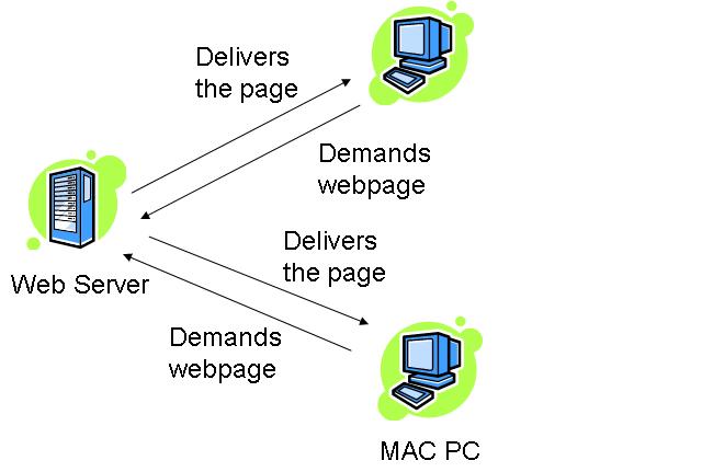

How this works??
The HTTP:TCP transport service uses sockets to transfer the data. The client initiates the TCP connection by using sockets on port 80 to the server. Then the server accepts the connection from the client. The client requests with the HTML pages and the objects which are then exchanged between the client browser and web server. After completing the request, the TCP connection is closed.
As HTTP is a stateless protocol. It does not keep user information about the previous client requests. So, this protocol is simple but if you have to maintain the past client records then it is complex. Since the server will maintain all the client requests and when the server crashes, it is very difficult to get the information back and makes the system very complex.
HTTP Connections[edit | edit source]
The web page consists of objects and URL’s. As there can be one or many objects or URL’s, the type of HTTP connection determines the order in which the objects are requested.
Since the HTTP is constantly evolving to improve its performance, there are two types of connections: • Non-Persistent (HTTP/1.0) • Persistent (HTTP/1.1)
The major difference between non-persistent and persistent connection is the number of TCP connection(s) required for transmitting the objects.
Non-Persistent HTTP – This connection requires that each object be delivered by an individually established TCP connection. Usually there is one round trip time delay for the initial TCP connection. Suppose user requests the page that contains text as well as 5 images. The number of TCP connections will be as follows:


Persistent HTTP -
This connection is also called as HTTP keep-alive, or HTTP Reuse. The idea is to use the same TCP connection to send and receive multiple HTTP requests/responses using the same connection. Using persistent connection is important to improve performance.
Persistent HTTP without Pipelining – In this connection, each client has to wait for the previously requested object received before issuing a new request for another object. Thus, not counting the initial TCP establishment (one RTT time), each object needs at least one RTT plus the transmission time of the object by the server.
Persistent HTTP with Pipelining – Can allow client to send out all (multiple) requests, so servers can receive all requests at once, and then sending responses (objects) one after another. The Pipelining method in HTTP/1.1 is default. The shortest time in pipelining is one initial RTT, RTT for request and response and the transmission time of all the objects by the server.
Thus, we can say that the number of RTT’s required in all the above types considering for some text and three objects would be:
- Non-persistent HTTP:
- Persistent HTTP
- Without Pipelining:
- With Pipelining:
Response Time (Modeling)[edit | edit source]
Round Trip Time (RTT): The time taken to send a packet to remote host and receive a response: used to measure delay on the network at a given time.
Response time:
The response time denotes the time required to initiate the TCP connection and the next response and requests to receive back along with the file transmission time.
The following example denotes the response time -


From the above fig. we can state that the response time is :
2 RTT + File transmit time.
HTTP Message Format :[edit | edit source]
There are two types of messages that HTTP uses – 1. Request message 2. Response message
1. Request Message:[edit | edit source]
The request line has three parts, separated by spaces: a method name, the local path of the requested resource and version of HTTP being used. The message format is in ASCII so that it can be read by the humans.
For e.g.:
GET /path/to/the/file.html HTTP/1.0
The GET method is the most commonly used. It states that “give me this resource”. The part of the URL is also called as Request URL. The HTTP is to be in uppercase and the next part denotes the version of HTTP.
HTTP Request Message: General Format
The HTTP Request message format is shown below:
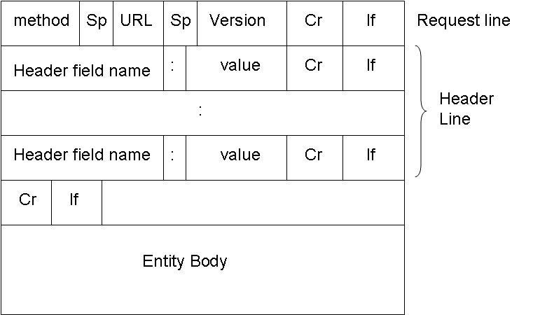

The method is the type of method used to request the URL. Like GET, POST or HEAD. The URL block contains the requested URL. Version denotes the HTTP version. Either HTTP/1.0 or HTTP/1.1. The header lines include the browser type, host , number of objects and file name and the type of language in the requested page. For e.g.:
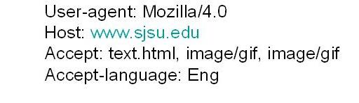

The entity body is used by the POST method. When user enters information on to the page, the entity body contains that information.
The HTTP 1.0 has GET, POST and HEAD methods. While the HTTP 1.1 has along with GET, POST and HEAD, PUT and DELETE.
Uploading the information in Web pages
The POST method
The Web pages which ask for input from user uses the POST method. The information filled by the web user is uploaded in server’s entity body.
The typical form submission in POST method. The content type is usually the application/x-www-form-urlencoded and the content-length is the length of the URL encoded form data.
The URL method
The URL method uses the GET method to get user input from the user. It appends the user information to be uploaded to server to the URL field.
2. Response Message:[edit | edit source]
The HTTP message response line also has three parts separated by spaces: the HTTP version, a response status code giving result of the request and English phrase of the status code. This first line is also called as Status line.
The HTTP Response message format is shown below:
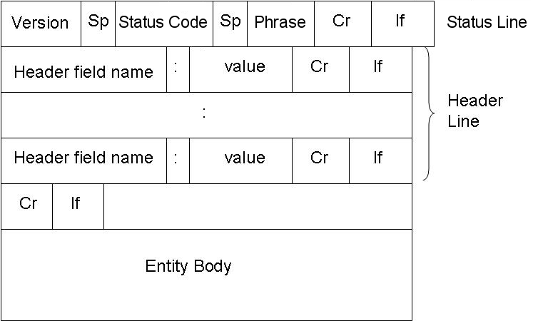

E.g.:
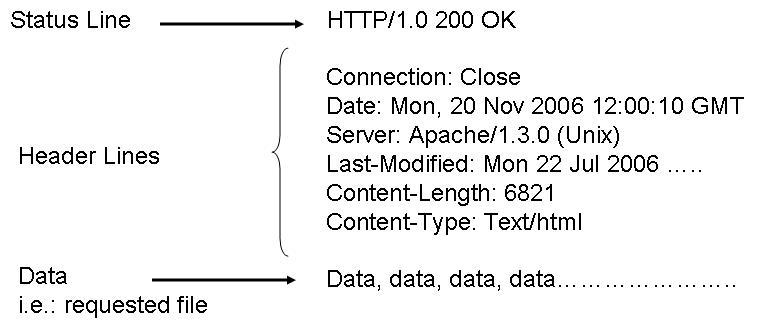

Below are the some HTTP response status codes:
200 OK The request succeeded, and the resulting resource (e.g. file or script output) is returned in the message body.
404 Not Found The requested resource doesn't exist.
301 Moved Permanently
302 Moved Temporarily
303 See Other (HTTP 1.1 only)
The resource has moved to another URL (given by the Location: response header), and should be automatically retrieved by the client. This is often used by a CGI script to redirect the browser to an existing file.
500 Server Error
An unexpected server error. The most common cause is a server-side script that has bad syntax, fails, or otherwise can't run correctly.
User Server Identification[edit | edit source]
The HTTP Protocol is a stateless protocol. So there should be an mechanism to identify the user using the web server. There are various techniques used:
1. Authentication 2. Cookies
1. Authentication:
The Client whenever request for the web page from the web server, the server authenticates the user. So each time whenever the web user or client requests any object, it has to provide a name and password to be identified by server. The need arises for the authentication so that the server has control over the documents. And, Since the HTTP protocol is stateless, it has to provide information each time it requests for web page. The authorization is done at the header line of the request. Generally, the cache is used to store the name and password of the web user. So that, each time it doesn’t have to provide the same information.
2. Cookies
Cookies are used by web servers to identify the web user. They are small piece of data stored into the web users disk. It is used in all major websites. As they have relatively much more importance in the web world. As said earlier, cookie is a small piece of data and not a code. This piece of small information is stored into web users machine whenever the browser visits the server site’s.
So how do the Cookie function exactly?
When the web users browser requests a file from web server, it send the file along with a cookie. So the next time whenever the web browser requests the same server a file, it sends the previous cookie to the web server so that it identifies that the browser had previously requested for a file. And so the web server coordinates your access to different pages from its website.
A typical example can be when you do online shopping., where cookie is used to traced your shopping basket .
The major four component of Cookie are:
1. Cookie header line in the HTTP response message. 2. Cookie header line in the HTTP request message. 3. Cookie file stored in User’s host and managed by User’s browser. 4. Back end database at the web site. So we can say that Cookies are used to keep the State of the web browser. Since HTTP is a stateless, so there should be some means for server to remember the state of the client’s request.
Cookies are in two flavors, one is persistent and the other is non-persistent. Persistent Cookies remain in the web browser’s machine memory for the specified time when it was first created. While non-persistent cookies are the ones which are deleted as soon as the web user’s browser is closed.
Cookies bring a number of useful applications in today’s Internet world. With the help of cookie, you can have: • User accounts • Online Shopping • Web Portals • Advertising
But with these cookies, you can secretly track down the web user’s habits. As whenever a web browser sends a request to web server, it includes its IP address, the type of browser you use and your operating system. So this information is also logged into the server’s file.
The Advertising is the main issue in cookies. Since, it is less admirable because of its use as a tracking of individual’s browsing and buying habits. As the server’s log file has all your information, so it becomes easier to track you. The advertisement firm has many clients which includes another several advertising firms. So it has contracts with many other agencies. They place an image file on their web site. Once you click on them, you are not clicking on the image but a link to another advertising firm’s site. So it sends a cookie to you when you request for that page. And thus, your IP address is tracked down. Whenever you request to their site’s page, they can track your number of visits to their site, which page you have visited and how often. Therefore, they come to know about your interests. So this important piece of information is valuable to them to track your preferences and target you based on your inferences.
Web Caching (Proxy Server) [edit | edit source]
The proxy server’s main goal is to satisfy client’s request without involving the original web server. It is a server acting like as a buffer between the Client’s web browser and the Web server. It accepts the requests from the user and responses to them if it contains the requested page. If it doesn’t have the requested page, then it requests to Original Web Server and responses to the client. It uses cache to store the pages. If the requested web page is in cache, it fulfills the request speedily.
Working of Proxy Server


The two main purpose of proxy server are:
1. Improve Performance –
As it saves the result for a particular period of time. If the same result is requested again and if it is present in the cache of proxy server then the request can be fulfilled in less time. So it drastically improves the performance. The major online searches do have an array of proxy servers to serve for a large number of web users.
2. Filter Requests -
Proxy server’s can also be used to filter requests. Suppose an company wants to restrict the user from accessing a specific set of sites, it can be done with the help of proxy servers.
Conditional GET
The conditional GET is the same as GET method. It only differs by including the If-modified-since, If-unmodified-since, If-match, If-None-Match or If-Range header field. The conditional GET method requests can be satisfied under the given conditions. This is method is used to reduce the network usage so that cache entities can be utilized to fulfill requests if they are not modified and avoids unnecessary transferring of data.
Working of Conditional GET:
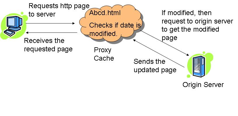

Whenever the client request to the server for html page, the proxy server checks the requested page in its cache. It checks the last-modified date entry in the header


If the requested page in the cache entry determined to be out of date, the proxy server requests the updated page from the main server. And then, the main server responds to that requests and sends updates to the page to the proxy server; which are then forwarded to the client, as well as stored in the proxy server cache.
HTTPS[edit | edit source]
The HTTPS is a secure version of HTTP. It indicates the port 443 should be used instead of port 80. It is widely used, both in security concern areas such as eCommerce, as well as crime prevention by attempting to make sure the end user is actually getting the sites he was looking for. The protocol identifier HTTPS instructs the user agent the user is looking for a secure channel.
The HTTPS follows a procedure to follow secure connection in the network. The secure connection is done automatically. The steps are:
- The client authenticates the server using the server’s digital certificate.
- The client and server negotiate with the cipher suite (a set of security protocols) they will use for the connection.
- The client and server generate session keys for encrypting and decrypting data.
- The Client and server establish a secure encrypted connection.
The HTTPS ends its session whenever the client or server cannot negotiate with the cipher suite. The cipher suite can be based on any of the following:
- Digest Based –
- Message Digest 5 (MD5)
- Secure Hash Algorithm 1 (SHA-1)
- Public Key-Based –
- Rivest-Shamir-Adelman (RSA) encryption/decryption.
- Digital Signature Algorithm (DSA)
- Diffie-Hellman Key-exchange/Key-generation.
- X.509 digital certificates.
SUMMARY[edit | edit source]
This chapter includes HTTP how the Web World is all about. The various methods used in TCP connection to transfer the data in the web world. It has detail information on requests and response methods. Also it contains the User Identification methods like Authentication and Cookies. The cookies part is explained in detail. Also the various connections in HTTP, like non-persistent and persistent connections. We have also mentioned about the proxy server and how does it works. And lastly, the secure version of HTTP.i.e. HTTPS.
File Transfer Protocol (FTP) is a standard network protocol used to exchange and manipulate files over a TCP/IP based network, such as the Internet. FTP is built on a client-server architecture and utilizes separate control and data connections between the client and server applications. FTP is also often used as an application component to automatically transfer files for program internal functions. FTP can be used with user-based password authentication or with anonymous user access.
Purpose[edit | edit source]
Objectives of FTP, as outlined by its RFC, are:
- To promote sharing of files (computer programs and/or data).
- To encourage indirect or implicit use of remote computers.
- To shield a user from variations in file storage systems among different hosts.
- To transfer data reliably, and efficiently.
- To grant readability to the end user.
Connection methods[edit | edit source]
FTP runs over the Transmission Control Protocol (TCP). Usually FTP servers listen on the well-known port number 21 (IANA-reserved) for incoming connections from clients. A connection to this port from the FTP client forms the control stream on which commands are passed to the FTP server and responses are collected. FTP uses out-of-band control; it opens dedicated data connections on other port numbers. The parameters for the data streams depend on the specifically requested transport mode. Data connections usually use port number 20.
In active mode, the FTP client opens a dynamic port, sends the FTP server the dynamic port number on which it is listening over the control stream and waits for a connection from the FTP server. When the FTP server initiates the data connection to the FTP client it binds the source port to port 20 on the FTP server.
In order to use active mode, the client sends a PORT command, with the IP and port as argument. The format for the IP and port is "h1,h2,h3,h4,p1,p2". Each field is a decimal representation of 8 bits of the host IP, followed by the chosen data port. For example, a client with an IP of 192.168.0.1, listening on port 49154 for the data connection will send the command "PORT 192,168,0,1,192,2". The port fields should be interpreted as p1×256 + p2 = port, or, in this example, 192×256 + 2 = 49154.
In passive mode, the FTP server opens a dynamic port, sends the FTP client the server's IP address to connect to and the port on which it is listening (a 16-bit value broken into a high and low byte, as explained above) over the control stream and waits for a connection from the FTP client. In this case, the FTP client binds the source port of the connection to a dynamic port.
To use passive mode, the client sends the PASV command to which the server would reply with something similar to "227 Entering Passive Mode (127,0,0,1,192,52)". The syntax of the IP address and port are the same as for the argument to the PORT command.
In extended passive mode, the FTP server operates exactly the same as passive mode, however it only transmits the port number (not broken into high and low bytes) and the client is to assume that it connects to the same IP address that was originally connected to.
While data is being transferred via the data stream, the control stream sits idle. This can cause problems with large data transfers through firewalls which time out sessions after lengthy periods of idleness. While the file may well be successfully transferred, the control session can be disconnected by the firewall, causing an error to be generated.
The FTP protocol supports resuming of interrupted downloads using the REST command. The client passes the number of bytes it has already received as argument to the REST command and restarts the transfer. In some commandline clients for example, there is an often-ignored but valuable command, "reget" (meaning "get again"), that will cause an interrupted "get" command to be continued, hopefully to completion, after a communications interruption.
Resuming uploads is not as easy. Although the FTP protocol supports the APPE command to append data to a file on the server, the client does not know the exact position at which a transfer got interrupted. It has to obtain the size of the file some other way, for example over a directory listing or using the SIZE command.
In ASCII mode (see below), resuming transfers can be troublesome if client and server use different end of line characters.
Data format[edit | edit source]
While transferring data over the network, several data representations can be used. The two most common transfer modes are:
- ASCII mode
- Binary mode: In "Binary mode", the sending machine sends each file byte for byte and as such the recipient stores the bytestream as it receives it. (The FTP standard calls this "IMAGE" or "I" mode)
In ASCII mode, any form of data that is not plain text will be corrupted. When a file is sent using an ASCII-type transfer, the individual letters, numbers, and characters are sent using their ASCII character codes. The receiving machine saves these in a text file in the appropriate format (for example, a Unix machine saves it in a Unix format, a Windows machine saves it in a Windows format). Hence if an ASCII transfer is used it can be assumed plain text is sent, which is stored by the receiving computer in its own format. Translating between text formats might entail substituting the end of line and end of file characters used on the source platform with those on the destination platform, e.g. a Windows machine receiving a file from a Unix machine will replace the line feeds with carriage return-line feed pairs. It might also involve translating characters; for example, when transferring from an IBM mainframe to a system using ASCII, EBCDIC characters used on the mainframe will be translated to their ASCII equivalents, and when transferring from the system using ASCII to the mainframe, ASCII characters will be translated to their EBCDIC equivalents.
By default, most FTP clients use ASCII mode. Some clients try to determine the required transfer-mode by inspecting the file's name or contents, or by determining whether the server is running an operating system with the same text file format.
The FTP specifications also list the following transfer modes:
- EBCDIC mode - this transfers bytes, except they are encoded in EBCDIC rather than ASCII. Thus, for example, the ASCII mode server
- Local mode - this is designed for use with systems that are word-oriented rather than byte-oriented. For example mode "L 36" can be used to transfer binary data between two 36-bit machines. In L mode, the words are packed into bytes rather than being padded. Some FTP servers accept "L 8" as being equivalent to "I".
In practice, these additional transfer modes are rarely used. They are however still used by some legacy mainframe systems.
The text (ASCII/EBCDIC) modes can also be qualified with the type of carriage control used (e.g. TELNET NVT carriage control, ASA carriage control), although that is rarely used nowadays.
Note that the terminology "mode" is technically incorrect, although commonly used by FTP clients. "MODE" in RFC 959 refers to the format of the protocol data stream (STREAM, BLOCK or COMPRESSED), as opposed to the format of the underlying file. What is commonly called "mode" is actually the "TYPE", which specifies the format of the file rather than the data stream. FTP also supports specification of the file structure ("STRU"), which can be either FILE (stream-oriented files), RECORD (record-oriented files) or PAGE (special type designed for use with TENEX). PAGE STRU is not really useful for non-TENEX systems, and RFC 1123 section 4.1.2.3 recommends that it not be implemented.
FTP return codes[edit | edit source]
FTP server return codes indicate their status by the digits within them. A brief explanation of various digits' meanings are given below:
- 1xx: Positive Preliminary reply. The action requested is being initiated but there will be another reply before it begins.
- 2xx: Positive Completion reply. The action requested has been completed. The client may now issue a new command.
- 3xx: Positive Intermediate reply. The command was successful, but a further command is required before the server can act upon the request.
- 4xx: Transient Negative Completion reply. The command was not successful, but the client is free to try the command again as the failure is only temporary.
- 5xx: Permanent Negative Completion reply. The command was not successful and the client should not attempt to repeat it again.
- x0x: The failure was due to a syntax error.
- x1x: This response is a reply to a request for information.
- x2x: This response is a reply relating to connection information.
- x3x: This response is a reply relating to accounting and authorization.
- x4x: Unspecified as yet
- x5x: These responses indicate the status of the Server file system vis-a-vis the requested transfer or other file system action.
Anonymous FTP[edit | edit source]
A host that provides an FTP service may additionally provide anonymous FTP access. Users typically login to the service with an 'anonymous' account when prompted for user name. Although users are commonly asked to send their email address in lieu of a password, little to no verification is actually performed on the supplied data.
As modern FTP clients typically hide the anonymous login process from the user, the ftp client will supply dummy data as the password (since the user's email address may not be known to the application). For example, the following ftp user agents specify the listed passwords for anonymous logins:
- Mozilla Firefox (3.0.7) —
mozilla@example.com - KDE Konqueror (3.5) —
anonymous@ - wget (1.10.2) —
-wget@ - lftp (3.4.4) —
lftp@
Commands[edit | edit source]
Enter ftp /? in Windows, or ftp --help in Unix, to get the command parameters.
Once connected to a server, type help to display the different possible commands.
To manipulate the files with the mouth, download a good FTP client which will do the interface (for example this Filezilla doesn't need any installation).
Routing[edit | edit source]
Routing is the process of getting information packets where they need to go. Routing is a surprisingly complicated task, and there are a number of different algorithms used to find the shortest route between two points.
Introduction[edit | edit source]
IP addressing is based on the concept of hosts and networks. A host is essentially anything on the network that is capable of receiving and transmitting IP packets on the network, such as a workstation or a router. Routing is a process of moving data from one host computer to another. The difference between routing and bridging is that bridging occurs at Layer 2 (the link layer) of the OSI reference model, whereas routing occurs at Layer 3 (the network layer). Routing determines the optimal routing paths through a network.
Routing Algorithms[edit | edit source]
The routing algorithm is stored in the router's memory. The routing algorithm is a major factor in the performance of your routing environment. The purpose of the routing algorithm is to make decisions for the router concerning the best paths for data. The router uses the routing algorithm to compute the path that would best serve to transport the data from the source to the destination. Note that you do not directly choose the algorithm that your router uses. Rather, the routing protocol you choose for your network determines which algorithm you will use. For example, whereas the routing protocol Routing Information Protocol (RIP) may use one type of routing algorithm to help the router move data, the routing protocol Open Shortest Path First (OSPF) uses another. The routing algorithm cannot be changed. The only way to change it is to change routing protocols. The overall performance of your network depends mainly on the routing algorithm, so you should research the algorithms each protocol uses before deciding which to implement on your network. There are two major categories of routing algorithms - distance vector or link-state. Every routing protocol named "distance vector" uses the distance vector algorithm, and every link-state protocol uses the link-state algorithm.
Routing Algorithms within Routing Protocols[edit | edit source]
One of the jobs of the routing protocol is to provide the information needed by the routing algorithm to compute its decisions. This is the point where many protocols differ. The information provided to the algorithm can be different from protocol to protocol.
The routing protocol gathers information about networks and routers from the surrounding environment and stores the information within a routing table in the router's memory. The routing algorithm is run using the information within this table to calculate the best path from one network to another. Calculating the new values within the formula then generates a sum. The result of this calculation is used then to determine where to send information. For example, the table below illustrates a sample routing table for a fictitious routing environment. The information that is passed to the routing algorithm within the routing table is gathered by the routing protocol through a process known as a routing update. Through a series of updates, each router will tell the other what information it has. Eventually, an entire routing table will be built.
| Router Link | Metric |
|---|---|
| Router A to Router B | 2 |
| Router B to Router C | 3 |
| Router A to Router C | 6 |
| Router C to Router D | 5 |
The sample routing algorithm states that the best path to any destination is the one that has the lowest metric value. A metric is a number that is used as a standard of measurement for the links of a network. Each link is assigned a metric to represent anything from monetary cost to use the line, to the amount of available bandwidth. When Router A is presented with a packet bound from Router C, the routing table shows two possible paths to choose from. The first choice is to send the packet from Router A directly over the link to Router C. The second option is to send the packet from Router A to Router B and then on to Router C. The routing algorithm is used to determine which option is best.
Some routing protocols might only provide one metric to the routing algorithm, whereas others might provide up to ten. On the other hand, whereas two protocols might both send only one metric to the algorithm, the origin of that metric might differ from protocol to protocol. One routing protocol might give an algorithm the single metric of cost, but that cost could represent something different than another protocol using the same metric.
The algorithm in our example states that the best path is the one with the lowest metric value. Therefore, by adding the metric numbers associated with each possible link, we see that the route from Router A to Router B to Router C has a metric value of 5, while the direct link to Router C has a value of 6. The algorithm selects the A-B-C path and sends the information along.
Distance Vector Algorithms[edit | edit source]

A distance vector algorithm uses metrics known as costs in order to help determine the best path to a destination. The path with the lowest total cost is chosen as the best path.
When a router utilizes a distance vector algorithm, different costs are gathered by each router. These costs can be completely arbitrary numbers. Costs can also be dynamically gathered values, such as the amount of delay experienced by routers when sending packets over one link as opposed to another. All the costs are compiled and placed within the router's routing table and then they are used by the algorithm to calculate a best path for any given network scenario.
Although there are many resources that will offer complex mathematical representations of what distance vector algorithms are and how they compute their decisions, the core concept remains the same - by adding the metrics for every optional path on a network, you will come up with at least one best path. The formula for this is as follows:
M(i,k) = min [M(i,t) + M(t,k)]
This formula states that the best path between two networks (M(i,k)) can be found by finding the lowest (min) value of paths between all network points. Let's look again at the routing information in the table above. Plugging this information into the formula, we see that the route from A to B to C is still the best path:
5(A,C) = min[2(A,B) + 3(B,C)]
Whereas the formula for the direct route A to C looks like this:
6(A,C) = min[6(A,C)]
This example shows how distance vector algorithms use the information passed to them to make informed routing decisions. The algorithms used by routers and routing protocols are not configurable, nor can they be modified.
Another major difference between distance vector algorithms and link state protocols is that when distance vector routing protocols update each other, all or part of the routing table (depending on the type of update) is sent from one router to another. By this process, each router is exposed to the information contained within the other router's tables, thus giving each router a more complete view of the networking environment and enabling them to make better routing decisions. Examples of distance vector algorithms include RIP and BGP, two of the more popular protocols in use today. Other popular protocols such as OSPF are examples of protocols which use the link state routing algorithm.
Distance vector algorithms are also known as Bellman-Ford routing algorithms and Ford-Fulkerson routing algorithms. In these algorithms, each router has a routing table which shows it the best route for any destination. A typical graph and routing table for router J is shown below.

| Destination | Weight | Line |
|---|---|---|
| A | 8 | A |
| B | 20 | A |
| C | 20 | I |
| D | 20 | H |
| E | 17 | I |
| F | 30 | I |
| G | 18 | H |
| H | 12 | H |
| I | 10 | I |
| J | 0 | N/A |
| K | 6 | K |
| L | 15 | K |
The table shows that if router J wants to get packets to router D, it should send them to router H first. When the packets arrive at router H, the current router checks its own table and makes a decision how to send the packets to D.
In distance vector algorithms, each router has to follow the following steps:
1. It counts the weight of the links directly connected to it and saves the information to its table.
2. In a particular period of time, the router sends its table to its neighbor routers (not to all routers) and receives the routing table of each of its neighbors.
3. Based on the information the router receives from its neighbors' routing tables, it updates its own.
Let's consider one more example (the figure represented below).

The cost of each link is set to 1. Thus, the least cost path is simply the path with the fewer hops. The table below represents each node knowledge about the distance to all other nodes:
| Information stored at node |
Distance to reach node | ||||||
|---|---|---|---|---|---|---|---|
| A | B | C | D | E | F | G | |
| A | 0 | 1 | 1 | 1 | 1 | ||
| B | 1 | 0 | 1 | ||||
| C | 1 | 1 | 0 | 1 | |||
| D | 1 | 0 | 1 | ||||
| E | 1 | 0 | |||||
| F | 1 | 0 | 1 | ||||
| G | 1 | 1 | 0 | ||||

Initially, each node sets a cost of 1 to its directly connected neighbors and infinity to all the other nodes. Below is shown the initial routing table at node A:
| Destination | Cost | Next Hop |
|---|---|---|
| B | 1 | B |
| C | 1 | C |
| D | - | |
| E | 1 | E |
| F | 1 | F |
| G | - |
During the next step, every node sends a message to its directly connected neighbors. That message contains the node's personal list of distances. Node F, for example, tells node A that it can reach node G at cost of 1; node A also knows that it can reach F at a cost of 1, so it adds these costs to get the cost of reaching G by means of F. Because 2 is less than the current cost of infinity, node A records that it can reach G at a cost of 2 by going trough F. Node A learns from C that node B can be reached from C at a cost of 1, so it concludes that the cost of reaching B via C is 2. Because this is worse than the current cost of reaching B, which is 1, the new information is ignored. The final routing table at node A is shown below:
| Destination | Cost | Next Hop |
|---|---|---|
| B | 1 | B |
| C | 1 | C |
| D | 2 | C |
| E | 1 | E |
| F | 1 | F |
| G | 2 | F |
The process of getting consistent routing information to all the nodes is called convergence. The final set of costs from each node to all other nodes is shown in the table below:
| Information stored at node |
Distance to reach node | ||||||
|---|---|---|---|---|---|---|---|
| A | B | C | D | E | F | G | |
| A | 0 | 1 | 1 | 2 | 1 | 1 | 2 |
| B | 1 | 0 | 1 | 2 | 2 | 2 | 3 |
| C | 1 | 1 | 0 | 1 | 2 | 2 | 2 |
| D | 2 | 2 | 1 | 0 | 3 | 2 | 1 |
| E | 1 | 2 | 2 | 3 | 0 | 2 | 3 |
| F | 1 | 2 | 2 | 2 | 2 | 0 | 1 |
| G | 2 | 3 | 2 | 1 | 3 | 1 | 0 |
The cost of each link is set to 1. Thus, the least cost path is simply the path with the fewer hops.
One of the problems with distance vector algorithms is called "count to infinity." Let's examine the following problem with an example:
Consider a network with a graph as shown below. There is only one link between D and the other parts of the network.

with vectors
d [A][A] = 0 d [A][B] = 1 d [A][C] = 2 d [A][D] = 3
| A | B | C | D | |
|---|---|---|---|---|
| A | 0 | 1 | 2 | 3 |
| B | 1 | 0 | 1 | 2 |
| C | 2 | 1 | 0 | 1 |
| D | 3 | 2 | 1 | 0 |
Now the C to D link crashes
So cost [C][D] = ∞
C used to forward any packets with address D directly on the CD link, but now link is down, so C has to recompute its distance vector (and make a new choice of how to forward packets to D) - similarly D has to update its vector. After updating their vectors at C and D, we have
| A | B | C | D | |
|---|---|---|---|---|
| A | 0 | 1 | 2 | 3 |
| B | 1 | 0 | 1 | 2 |
| C | 2 | 1 | 0 | 3 |
| D | 0 |
C views B as the best route to D, with cost 1 + 2, so C sends new vector to B. B learns that its former choice for sending to D via C now has higher cost, so B should recompute its vector.
| A | B | C | D | |
|---|---|---|---|---|
| A | 0 | 1 | 2 | 3 |
| B | 1 | 0 | 1 | 4 |
| C | 2 | 1 | 0 | 3 |
| D | 0 |
View of B is that routing to D can either go via A or C with equal cost - B sends updated vector. Both A and C get updated vector from B and learn that their preferred route to D now has higher cost, so they recompute their own vectors.
| A | B | C | D | |
|---|---|---|---|---|
| A | 0 | 1 | 2 | 5 |
| B | 1 | 0 | 1 | 4 |
| C | 2 | 1 | 0 | 5 |
| D | 0 |
Then A and C send their vectors, B has to update its vector again, sending another round to A and C, obtaining.
| A | B | C | D | |
|---|---|---|---|---|
| A | 0 | 1 | 2 | 7 |
| B | 1 | 0 | 1 | 6 |
| C | 2 | 1 | 0 | 7 |
| D | 0 |
Notice that the routing table is very slowly converging to the fact that
d [x][D] = ∞ for x = A or x = B or x = C
This process loops until all nodes find out that the weight of link to D is infinity. In this way, experts say that distance vector algorithms have a slow convergence rate. In conclusion, distance vector algorithm is not robust. One way to solve this problem is for routers to send information only to the neighbors that are not exclusive links to the destination. For example, in this case, B should not send any information to C about D, because C is the only way to D.
Link-State Algorithms[edit | edit source]

Distance vector algorithms and link-state algorithms both favor the path with the lowest cost. However, link-state protocols work in more localized manner. Whereas a router running a distance vector algorithm will compute the end-to-end path for any given packet, a link-state protocol will compute that path as it relates to the most immediate link. That is, where a distance vector algorithm will compute the lowest metric between Network A and Network C, a link-state protocol will compute it as two distinct paths, A to B and B to C.
This process is very efficient for larger environments. Link-state algorithms enable routers to focus on their own links and interfaces. Any one router on a network will only have direct knowledge of the routers and networks that are directly connected to it (or, the state of its own links). In larger environments, this means that the router will use less processing power to compute complicated paths.
The router simply needs to know which one of its direct interfaces will get the information where it needs to go the quickest. The next router in line will repeat the process until the information reaches its destination.
Another advantage to such localized routing processes is that protocols can maintain smaller routing tables. Because a link-state protocol only maintains routing information for its direct interfaces, the routing table contains much less information than that of a distance vector protocol that might have information for multiple routers.
Like distance vector protocols, link-state protocols require updates to share information with each other. These routing updates, known as Link State Advertisements (LSAs), occur when the state of a router's links changes.
When a particular link becomes unavailable (changes state), the router sends an update through the environment alerting all the routers with which it is directly linked.
In Link-State Algorithms, every router has to follow these steps:
1. Identify the routers that are physically connected to them and get their IP addresses
When a router starts working, it first sends a "HELLO" packet over network. Each router that receives this packet replies with a message that contains its IP address.
2. Routers measure the delay time (or any other important parameters of the network, such as average traffic) for neighbor routers. In order to do that, routers send echo packets over the network. Every router that receives these packets replies with an echo reply packet. By dividing round trip time by 2, routers can count the delay time. The delay time includes both transmission and processing times - the time it takes the packets to reach the destination and the time it takes the receiver to process it and reply.
3. Broadcast its information over the network for other routers and receive the other routers' information. In this step, all routers share their knowledge and broadcast their information to each other. In this way, every router can know the structure and status of the network.
4. Routers use an appropriate algorithm to identify the best route between two nodes of the network. In this step, routers choose the best route to every node. They do this using an algorithm, such as the Dijkstra shortest path algorithm. In this algorithm, a router, based on information that has been collected from other routers, builds a graph of the network. This graph shows the location of routers in the network and their links to each other. Every link is labeled with a number called the weight or cost. This number is a function of delay time, average traffic, and sometimes simply the number of hops between nodes. For example, if there are two links between a node and a destination, the router chooses the link with the lowest weight.
Dijkstra algorithm[edit | edit source]
The Dijkstra algorithm goes through the following steps:
- The router builds a graph of the network. Then it identifies source and destination nodes, for example R1 and R2. The router builds then a matrix, called the "adjacency matrix." In the adjacent matrix, a coordinate indicates weight. [i, j], for example, is the weight of a link between nodes Ri and Rj. If there is no direct link between Ri and Rj, this weight is identified as "infinity."
- The router then builds a status record for each node on the network. The record contains the following fields:
- Predecessor field - shows the previous node.
- Length field - shows the sum of the weights from the source to that node.
- Label field - shows the status of node; each node have one status mode: "permanent" or "tentative."
- In the next step, the router initializes the parameters of the status record (for all nodes) and sets their label to "tentative" and their length to "infinity".
- During this step, the router sets a T-node. If R1 is to be the source T-node, for example, the router changes R1's label to "permanent." Once a label is changed to "permanent," it never changes again.
- The router updates the status record for all tentative nodes that are directly linked to the source T-node.
- The router goes over all of the tentative nodes and chooses the one whose weight to R1 is lowest. That node is then the destination T-node.
- If the new T-node is not R2 (the intended destination), the router goes back to step 5.
- If this node is R2, the router extracts its previous node from the status record and does this until it arrives at R1. This list of nodes shows the best route from R1 to R2.

Dijkstra algorithm example:
Let’s find the best route between routers A and E. There are six possible routes between them (ABE, ACE, ABDE, ACDE, ABDCE, ACDBE), and it's obvious that ABDE is the best route because its weight is the lowest. But life is not always so easy, and there are some complicated cases in which we have to use algorithms to find the best route.
1. The source node (A) has been chosen as T-node, and so its label is permanent (permanent nodes are showed with filled circles and T-nodes with the -> symbol).

2. In this step, the status record of tentative nodes directly linked to T-node (B, C) has been changed. Also, because B has less weight, it has been chosen as T-node and its label has changed to permanent.

3. Like in step 2, the status records of tentative nodes that have a direct link to T-node (D, E), have been changed. Because router D has less weight, it has been chosen as T-node and its label has changed to permanent.

4. Because we do not have any tentative nodes, we just identify the next T-node. Because node E has the least weight, it has been chosen as T-node.
Now we have to identify the route. The previous node of E is node D, and the previous node of D is node B, and B's previous node is node A. So, we determine that the best route is ABDE. In this case, the total weigh is 4 (1+2+1). This algorithm works well, but it is so complicated that it may take a long time for routers to process it. That would cause the efficiency of the network to fail. Another note we should make here is that if a router gives the wrong information to other routers, all routing decisions will be ineffective.
The next example shows how to find the best routes among all the nodes in a network. The example uses the Shortest Path Dijkstra algorithm. Consider the network shown below:

Let's use the Dijkstra's algorithm to find the routes that A will use to transmit to any of the notes on the network. The Dijkstra's routing algorithm is represented in the following table:
| B | C | D | E | F | G | H | I | ||
|---|---|---|---|---|---|---|---|---|---|
| Step 1 | A | 2-A | 3-A | 5-A | |||||
| Step 2 | AB | 3-A | 5-A | 7-B | 9-B | ||||
| Step 3 | ABC | 4-C | 4-C | 9-B | |||||
| Step 4 | ABCD | 4-C | 9-B | 11-D | |||||
| Step 5 | ABCDE | 8-E | 12-E | 7-E | |||||
| Step 6 | ABCDEH | 8-E | 12-E | 11-H | |||||
| Step 7 | ABCDEHF | 10-F | 11-H | ||||||
| Step 8 | ABCDEHFG | 11-H | |||||||
| Step 9 | ABCDEHFGI |
This is how the network looks after all the updates, showing the shortest route among the nodes:

Interior Routing[edit | edit source]
Packet routing in the Internet is divided into two general groups: interior and exterior routing. Interior routing happens inside or interior to an independent network system. In TCP/IP terminology, these independent network systems are called autonomous systems. Within an autonomous system (AS), routing information is exchanged using an interior routing protocol chosen by the autonomous system's administration. The exterior routing protocols, on the other hand are used between the autonomous systems. Interior routing protocols determine the "best" route to each destination, and they distribute routing information among the systems on a network. There are several interior protocols:
- The Routing Information Protocol (RIP) is the interior protocol most commonly used on UNIX systems. RIP uses distance vector algorithm that selects the route with the lowest "hop count" (metric) as the best route. The RIP hop count represents the number of gateways through which data must pass to reach its destination. RIP assumes that the best route is the one that uses the fewest gateways.
- Hello is a protocol that uses delay as the deciding factor when choosing the best route. Delay is the length of time it takes a datagram to make the round trip between its source and destination.
- Intermediate System to Intermediate System (IS-IS) is an interior routing protocol from the OSI protocol suite. It is a link-state protocol. It was the interior routing protocol used on the T1 NSFNET backbone.
- Open Shortest Path First (OSPF) is another link-state protocol developed for TCP/IP. It is suitable for very large networks and provides several advantages over RIP.
Routing Information Protocol (RIP)[edit | edit source]
RIP (Routing Information Protocol) is a standard for exchange of routing information among gateways and hosts. It is a distance-vector protocol. RIP is most useful as an "interior gateway protocol". The network is organized as a collection of "autonomous systems". Each autonomous system has its own routing technology, which may well be different for different autonomous systems. The routing protocol used within an autonomous system is referred to as an interior gateway protocol, or "IGP". Routing Information Protocol (RIP) is designed to work with moderate-size networks using reasonably homogeneous technology. Thus, it is suitable as an Interior Gateway Protocol (IGP) for many campuses and for regional networks using serial lines whose speeds do not vary widely. It is not intended for use in more complex environments. RIP2 derives from RIP, which is an extension of the Routing Information Protocol (RIP) intended to expand the amount of useful information carried in the RIP messages and to add a measure of security. RIP2 is an UDP-based protocol.
What makes RIP work is a routing database that stores information on the fastest route from computer to computer, an update process that enables each router to tell other routers which route is the fastest from its point of view, and an update algorithm that enables each router to update its database with the fastest route communicated from neighboring routers:
Database - Each RIP router on a given network keeps a database that stores the following information for every computer in that network:
IP Address - The Internet Protocol address of the computer.
Gateway - The best gateway to send a message addressed to that IP address.
Distance - The number of routers between this router and the router that can send the message directly to that IP address.
Route change flag - A flag that indicates that this information has changed, used by other routers to update their own databases.
Timers - Various timers.
Algorithm - The RIP algorithm works like this:
Update - At regular intervals each router sends an update message describing its routing database to all the other routers that it is directly connected to. Some routers will send this message as often as every 30 seconds, so that the network will always have up-to-date information to quickly adapt to changes as computers and routers come on and off the network. The Protocol Structure for RIP & and RIP2 is shown in the figure below:
The Protocol Structure for RIP & and RIP2 is shown in the figure below:
| 8 bits | 16 bits | 32 bits |
|---|---|---|
| Command | Version | Unused |
| Address Family Identifier | Route Tag (only for RIP2; 0 for RIP) | |
| IP Address | ||
| Subnet Mask (only for RIP2; 0 for RIP) | ||
| Next Hop (only for RIP2; 0 for RIP) | ||
| Metric | ||
Command - The command field is used to specify the purpose of the datagram. There are five commands: Request, Response, Traceon (obsolete), Traceoff (obsolete) and Reserved.
Version - The RIP version number. The current version is 2.
Address family identifier - Indicates what type of address is specified in this particular entry. This is used because RIP2 may carry routing information for several different protocols. The address family identifier for IP is 2.
Route tag - Attribute assigned to a route which must be preserved and readvertised with a route. The route tag provides a method of separating internal RIP routes (routes for networks within the RIP routing domain) from external RIP routes, which may have been imported from an EGP or another IGP.
IP address - The destination IP address.
Subnet mask - Value applied to the IP address to yield the non-host portion of the address. If zero, then no subnet mask has been included for this entry.
Next hop - Immediate next hop IP address to which packets to the destination specified by this route entry should be forwarded.
Metric - Represents the total cost of getting a datagram from the host to that destination. This metric is the sum of the costs associated with the networks that would be traversed in getting to the destination.
Open Shortest Path First Protocol (OSPF)[edit | edit source]
OSPF is an interior gateway protocol used for between routers that belong to a single Autonomous System. OSPF uses link-state technology in which routers send each other information about the direct connections and links which they have to other routers. Each OSPF router maintains an identical database describing the Autonomous System’s topology. From this database, a routing table is calculated by constructing a shortest- path tree. OSPF recalculates routes quickly in the face of topological changes, utilizing a minimum of routing protocol traffic. An area routing capability is provided, enabling an additional level of routing protection and a reduction in routing protocol traffic. In addition, all OSPF routing protocol exchanges are authenticated. OSPF routes IP packets based solely on the destination IP address found in the IP packet header. IP packets are routed "as is" - they are not encapsulated in any further protocol headers as they transit the Autonomous System. OSPF allows sets of networks to be grouped together. Such a grouping is called an area. The topology of an area is hidden from the rest of the Autonomous System. This information hiding enables a significant reduction in routing traffic. Also, routing within the area is determined only by the area’s own topology, lending the area protection from bad routing data.
The OSPF algorithm works as described below:
Startup - When a router is turned on it sends Hello packets to all of its neighbors, receives their Hello packets in return, and establishes routing connections by synchronizing databases with adjacent routers that agree to synchronize.
Update - At regular intervals each router sends an update message called its "link state" describing its routing database to all the other routers, so that all routers have the same description of the topology of the local network.
Shortest path tree - Each router then calculates a mathematical data structure called a "shortest path tree" that describes the shortest path to each destination address and therefore indicates the closest router to send to for each communication; in other words - "open shortest path first".
The Protocol Structure of OSPF (Open Shortest Path First version 2) is shown below:
| 8 bits | 16 bits | 24 bits |
|---|---|---|
| Version No. | Packet Type | Packet Length |
| Router ID | ||
| Area ID | ||
| Checksum | AuType | |
| Authentication | ||
Version number - Protocol version number (currently 2).
Packet type - Valid types are as follows: 1 Hello 2 Database Description 3 Link State Request 4 Link State Update 5 Link State Acknowledgment.
Packet length - The length of the protocol packet in bytes. This length includes the standard OSPF header.
Router ID - The router ID of the packet’s source. In OSPF, the source and destination of a routing protocol packet are the two ends of an (potential) adjacency.
Area ID - identifying the area that this packet belongs to. All OSPF packets are associated with a single area. Most travel a single hop only.
Checksum - The standard IP checksum of the entire contents of the packet, starting with the OSPF packet header but excluding the 64-bit authentication field.
AuType - Identifies the authentication scheme to be used for the packet.
Authentication - A 64-bit field for use by the authentication scheme.
Intermediate System to Intermediate System Routing Protocol(IS-IS)[edit | edit source]
Intermediate System-to-Intermediate System (IS-IS) is a link-state protocol where IS (routers) exchange routing information based on a single metric to determine network topology. It behaves similar to Open Shortest Path First (OSPF) in the TCP/IP network. In an IS-IS network, there are End Systems, Intermediate Systems, Areas and Domains. End systems are user devices. Intermediate systems are routers. Routers are organized into local groups called "areas", and several areas are grouped together into a "domain". IS-IS is designed primarily providing intra-domain routing or routing within an area. IS-IS, working in conjunction with CLNP, ES-IS, and IDRP, provides complete routing over the entire network. IS-IS routing makes use of two-level hierarchical routing. Level 1 - routers know the topology in their area, including all routers and hosts, but they do not know the identity of routers or destinations outside of their area. Level 1 routers forward all traffic for destinations outside of their area to a level 2 router within their area which knows the level 2 topology. Level 2 routers do not need to know the topology within any level 1 area, except to the extent that a level 2 router may also be a level 1 router within a single area. IS-IS has been adapted to carry IP network information, which is called Integrated IS-IS. Integrated IS-IS has the most important characteristic necessary in a modern routing protocol: It supports VLSM and converges rapidly. It is also scalable to support very large networks. There are two types of IS-IS addresses: Network Service Access Point (NSAP) - NSAP addresses identify network layer services, one for each service running. Network Entity Title (NET) - NET addresses identify network layer entities or processes instead of services. Devices may have more than one of each of the two types of addresses. However NET’s should be unique and the System ID portion of the NSAP must be unique for each system. The Protocol Structure of IS-IS (Intermediate System to Intermediate System Routing Protocol) is shown below:
| 8 bits | 16 bits | |||
|---|---|---|---|---|
| Intradomain routing protocol discriminator | Length Indicator | |||
| Version/Protocol ID Extension | ID Length | |||
| R | R | R | PDU Type | Version |
| Reserved | Maximum Area Address | |||
Intra-domain routing protocol discriminator - Network layer protocol identifier assigned to this protocol
Length indicator - Length of the fixed header in octets.
Version/protocol ID extension - Equal to 1.
ID length - Length of the ID field of NSAP addresses and NETs used in this routing domain.
R - Reserved bits.
PDU type - Type of PDU. Bits 6, 7 and 8 are reserved.
Version - Equal to 1.
Maximum area addresses - Number of area addresses permitted for this intermediate systems area.
The format of NSAP for IS-IS is shown below:
| <-IDP-> | <-DSP-> | |||
|---|---|---|---|---|
| <-HO-DSP-> | ||||
| AFI | IDI | Contents assigned by authority identified in IDI field | ||
| <-Area Address-> | <-ID-> | <-SEL-> | ||
IDP - Initial Domain Part
AFI - Authority and Format Identifier (1-byte); Provides information about the structure and content of the IDI and DSP fields.
IDI - Initial Domain Identifier (variable length)
DSP - Domain Specific Part
HO-DSP - High Order Domain Specific Part
Area Address (variable)
ID - System ID 1- 8 bytes
SEL - n-selector (1-byte value that serves a function similar to the port number in Internet Protocol).
Exterior Routing[edit | edit source]
Exterior routing occurs between autonomous systems, and is of concern to service providers and other large or complex networks. The basic routable element is the Autonomous System.While there may be many different interior routing scheme, a single exterior routing system manages the global Internet, based primarily on the BGP-4 exterior routing protocol.
Border Gateway Protocol (BGP)[edit | edit source]
The Border Gateway Protocol (BGP) ensures that packets get to their destination network regardless of current network conditions. BGP is essentially a distance-vector algorithm, but with several added twists. First, BGP router establishes connections with the other BGP routers with which it directly communicates. The first thing it does is download the entire routing table of each neighboring router. After that it only exchanges much shorter update messages with other routers. BGP routers send and receive update messages to indicate a change in the preferred path to reach a computer with a given IP address. If the router decides to update its own routing tables because this new path is better, then it will subsequently propagate this information to all of the other neighboring BGP routers to which it is connected, and they will in turn decide whether to update their own tables and propagate the information further.
BGP uses the TCP/IP protocol on port 179 to establish connections. It has strong security features, including the incorporation of a digital signature in all communications between BGP routers. Each BGP router contains a Routing Information Base (RIB) that contains the routing information maintained by that router. The RIB contains three types of information:
- Adj-RIBs-In - The unedited routing information sent by neighboring routers.
- Loc-RIB - The actual routing information the router uses, developed from Adj-RIBs-In.
- Adj-RIBs-Out - The information the router chooses to send to neighboring routers.
BGP routers exchange information using four types of messages:
- Open - Used to open an initial connection with a neighboring router.
- Update - These messages do most of the work, exchanging routing information between neighboring routers, and contain one of the following pieces of information:
- Withdrawn routes - The IP addresses of computers that the router no longer can route messages to.
- Paths - A new preferred route for an IP address. This path consists of two pieces of information - the IP address, and the address of the next router in the path that is used to route messages destined for that address.
- Notification - Used to indicate errors, such as an incorrect or unreadable message received, and are followed by an immediate close of the connection with the neighboring router.
- Keepalive - Each BGP router sends a 19 byte Keepalive message to each neighboring router to let them know that it is still operational about every 30 seconds, and no more often than every three seconds. If any router does not receive a Keepalive message from a neighboring router within a set amount of time, it closes its connection with that router, and removes it from its Routing Information Base, repairing what it perceives as damage to the network.
Routing messages are the highest precedence traffic on the Internet, and each BGP router gives them first priority over all other traffic. This makes sense - if routing information can't make it through, then nothing else will.
The BGP algorithm is run after a BGP router receives an update message from a neighboring router, and consists of the following three steps performed for each IP address sent from the neighbor:
- Update - If the path information for an IP address in the update message is different from the information previously received from that router, then the Adj-RIBs-In database is updated with the newest information.
- Decision - If it was new information, then a decision process is run that determines which BGP router, of all those presently recorded in the Adj-RIBs-In database, has the best routing path for the IP address in the update message. The algorithm is not mandated, and BGP administrators can set local policy criteria for the decision process such as how long it takes to communicate with each neighboring router, and how long each neighboring router takes to communicate with the next router in the path. If the best path chosen as a result of this decision process is different from the one currently recorded in the Loc-RIB database, then the database is updated.
- Propagation - If the decision process found a better path, then the Adj-RIBs-Out database is updated as well, and the router sends out update messages to all of its neighboring BGP routers to tell them about the better path. Each neighboring router then runs their own BGP algorithm in turn, decides whether or not to update their routing databases, and then propagates any new and improved paths to neighboring routers in turn.
One of the other important functions performed by the BGP algorithm is to eliminate loops from routing information. For example, a routing loop would occur when router A thinks that router B has the best path to send messages for some computer and B thinks the best path is through C, but C thinks the best path is back through A. If these sort of routing loops were allowed to happen, then any message to that computer that passed through routers A, B, or C would circulate among them forever, failing to deliver the message and using up increasing amounts of network resources. The BGP algorithm traps and stops any such loops.
Hierarchical Routing[edit | edit source]
In both Link-State and Distance Vector algorithms, every router has to save some information about other routers. When the network size grows, the number of routers in the network increases. As a result, the size of routing tables increases, as well, and routers can not handle network traffic as efficiently. Hierarchical routing are used to overcome this problem. Let us examine an example:
Distance Vector algorithms algorithms are used to find best routes between nodes. In the situation depicted below, every node of the network has to save a routing table with 17 records.

Here is a typical graph and routing table for A:
| Destination | Line | Weight |
|---|---|---|
| A | N/A | N/A |
| B | B | 1 |
| C | C | 1 |
| D | B | 2 |
| E | B | 3 |
| F | B | 3 |
| G | B | 4 |
| H | B | 5 |
| I | C | 5 |
| J | C | 6 |
| K | C | 5 |
| L | C | 4 |
| M | C | 4 |
| N | C | 3 |
| O | C | 4 |
| P | C | 2 |
| Q | C | 3 |
In hierarchical routing, routers are classified in groups known as regions. Each router has only the information about the routers in its own region and has no information about routers in other regions. That way, routers just save one record in their table for every other region. In this example, we have classified our network into five regions (see below).

| Destination | Line | Weight |
|---|---|---|
| A | N/A | N/A |
| B | B | 1 |
| C | C | 1 |
| Region 2 | B | 2 |
| Region 3 | C | 4 |
| Region 4 | C | 3 |
| Region 5 | C | 2 |
If A wants to send packets to any router in region 2 (D, E, F or G), it sends them to B, and so on. As you can see, in this type of routing, the tables can be summarized, so network efficiency improves. The above example shows two-level hierarchical routing. We can also use three-level or four-level hierarchical routing.
In three-level hierarchical routing, the network is classified into a number of clusters. Each cluster is made up of a number of regions, and each region contains a number or routers. Hierarchical routing is widely used in Internet routing and makes use of several routing protocols.
Summary[edit | edit source]
In Distance Vector Algorithms send everything you know to your neighbors, since Link-State Algorithms send info about your neighbors to everyone.
The Message size is small with Link-State Algorithms, and it is potentially large with Distance Vector Algorithms
The message exchange is large in Link-State Algorithms, while in Distance Vector Algorithms, the exchangement is only to neighbors
Convergence speed:
– Link-State Algorithms: fast
– Distance Vector Algorithms: fast with triggered updates
Space requirements:
– Link-State Algorithms maintains entire topology
– Distance Vector Algorithms maintains only neighbor state
Robustness:
• Link-State Algorithms can broadcast incorrect/corrupted LSP – localized problem
• Distance Vector Algorithms can advertise incorrect paths to all destinations – incorrect calculation can spread to entire network
Exercises[edit | edit source]
1. For the network given below, give global distance-vector tables when
a) each node knows only the distances to its immediate neighbors
b) each node has reported the information it had in the preceding step to its immediate neighbors
c) step b) happens a second time

2. For the network in exercise 1, show how the link-state algorithm builds the routing vector table
for node D.
3. For the network given in the figure below, give global distance-vector tables when
a) each node knows only the distances to its immediate neighbors
b) each node has reported the information it had in the preceding step to its immediate neighbors
c) step b) happens a second time

4. Suppose we have the forwarding tables shown below for nodes A and F, in a network where all links have cost 1. Give a diagram of the smallest network consistent with these tables.
For node A we have:
| Node | Cost | Next Hop |
|---|---|---|
| B | 1 | B |
| C | 1 | C |
| D | 2 | B |
| E | 3 | C |
| F | 2 | C |
For node F we have:
| Node | Cost | Next Hop |
|---|---|---|
| A | 2 | C |
| B | 3 | C |
| C | 1 | C |
| D | 2 | C |
| E | 1 | E |
5. For the network below, find the least cost routes from node A as a source using the Shortest Path Dijkstra's algorithm.

Answers[edit | edit source]
1.
a)
| Information stored at node |
Distance to reach node | |||||
|---|---|---|---|---|---|---|
| A | B | C | D | E | F | |
| A | 0 | 3 | 8 | |||
| B | 0 | 2 | ||||
| C | 3 | 0 | 1 | 6 | ||
| D | 8 | 0 | 2 | |||
| E | 2 | 1 | 2 | 0 | ||
| F | 6 | 0 | ||||
b)
c)
| Information stored at node |
Distance to reach node | |||||
|---|---|---|---|---|---|---|
| A | B | C | D | E | F | |
| A | 0 | 6 | 3 | 6 | 4 | 9 |
| B | 6 | 0 | 3 | 4 | 2 | 9 |
| C | 3 | 3 | 0 | 3 | 1 | 6 |
| D | 6 | 4 | 3 | 0 | 2 | 9 |
| E | 4 | 2 | 1 | 2 | 0 | 7 |
| F | 9 | 9 | 6 | 9 | 7 | 0 |
2.
| D | Confirmed | Tentative |
|---|---|---|
| 1. | (D,0,-) | |
| 2. | (D,0,-) | (A,8,A) (E,2,E) |
| 3. | (D,0,-) (E,2,E) (C,3,E) |
(A,8,A) (B,4,E) |
| 4. | (D,0,-) (E,2,E) (C,3,E) |
(A,6,E) (B,4,E) (F,9,E) |
| 5. | (D,0,-) (E,2,E) (C,3,E) (B,4,E) |
(A,6,E) (F,9,E) |
| 6. | previous + (A,6,E) | |
| 7. | previous + (F,9,E) | |
3.
a)
| Information stored at node |
Distance to reach node | |||||
|---|---|---|---|---|---|---|
| A | B | C | D | E | F | |
| A | 0 | 2 | 5 | |||
| B | 2 | 0 | 2 | 1 | ||
| C | 2 | 0 | 2 | 3 | ||
| D | 5 | 2 | 0 | |||
| E | 1 | 0 | 3 | |||
| F | 3 | 3 | 0 | |||
b)
| Information stored at node |
Distance to reach node | |||||
|---|---|---|---|---|---|---|
| A | B | C | D | E | F | |
| A | 0 | 2 | 4 | 5 | 3 | |
| B | 2 | 0 | 2 | 4 | 1 | 4 |
| C | 4 | 2 | 0 | 2 | 3 | 3 |
| D | 5 | 4 | 2 | 0 | 5 | |
| E | 3 | 1 | 3 | 0 | 3 | |
| F | 4 | 3 | 5 | 3 | 0 | |
c)
| Information stored at node |
Distance to reach node | |||||
|---|---|---|---|---|---|---|
| A | B | C | D | E | F | |
| A | 0 | 2 | 4 | 5 | 3 | 6 |
| B | 2 | 0 | 2 | 4 | 1 | 4 |
| C | 4 | 2 | 0 | 2 | 3 | 3 |
| D | 5 | 4 | 2 | 0 | 5 | 5 |
| E | 3 | 1 | 3 | 5 | 0 | 3 |
| F | 6 | 4 | 3 | 5 | 3 | 0 |
4.

5.
Step 1:

Step 2:

Step 3:

Step 4:

Step 5:

References[edit | edit source]
- http://e-books.amagrammer.net/
- Computer Networks, 3rd Ed., 2003, Peterson and Davie
- http://www.eng.ucy.ac.cy/christos/Courses/ECE360/Lectures.htm
Coding and Security[edit | edit source]
Basic Coding[edit | edit source]
It turns out that we can actually improve the performance of our system simply by changing the bits in our system. We can change the order of bits, or we can change the number of bits that we send, to help decrease error rates. This chapter will talk about transmission codes that can help increase system performance.
Gray Codes[edit | edit source]
Let us look at a basic QASK system:
- "00" = +5V
- "01" = +1.66V
- "10" = -1.66V
- "11" = -5V
We will call these "symbol 1" (for 00), "symbol 2" (for 01), "symbol 3" (for 10) and "symbol 4" (for 11).
Now, let us make a basic assumption that the only errors we get will be errors between adjacent symbols. For instance, Symbol 1 can be mistaken for symbol 2, but symbol 1 can never be mistaken for symbol 3. In reality, there is always a very small chance that this could happen, but we will simply ignore it for our purposes.
Now, we have 6 error conditions:
- Symbol 1 looks like Symbol 2
- Symbol 2 looks like Symbol 1
- Symbol 2 looks like Symbol 3
- Symbol 3 looks like Symbol 2
- Symbol 3 looks like Symbol 4
- Symbol 4 looks like Symbol 3
We can also see that in error conditions 1, 2, 5, and 6, a symbol error only produces 1 bit error. The other bit is actually not transmitted in error. The only time where we see 2 bits transmitted in error is when there is a mixup between symbols 2 and 3. We can calculate our probability of bit error as such:

Pone bit error is the probability that 1 bit from the symbol will be in error. Ptwo bits error is the probability that both symbols will be received in error.
To alleviate this problem, we can reorder our symbols, and map them the following way:
- "00" = +5V
- "01" = +1.66V
- "11" = -1.66V
- "10" = -5V
Now, when any symbol is received in error, there is only one bit error. This small trick is called "Gray Coding", and is a useful (but simple) method to improve system performance in terms of net bit errors.
Using Gray Codes[edit | edit source]
Gray codes are a simple example of how using an encoding/decoding mechanism in a communications system can have an effect on the error rate of the system. In future chapters we will discuss error correction codes (ECC) that can be used to find and fix single-bit errors in a signal. If we use Gray codes to ensure that the majority of errors are single-bit errors, we can then use more advanced ECC codes to resolve these errors.
Gray codes are typically not used on their own, but are combined with more robust coding methods, like described above.
For further reading[edit | edit source]
Spread Spectrum[edit | edit source]
There are multiple ways in which multiple clients can share a single transmission medium. Time-Division Multiplexing (TDM) is the system where different clients get "time slices", periods of time where one client gets to transmit and other clients cannot. Since nobody else is transmitting, each client gets to use the entire spectrum, which means high bandwidth and a fast data rate. There is also Frequency-Division Multiplexing (FDM), where each client transmits at the same time, but on different frequencies. In FDM there is less available bandwidth, but each client gets to transmit for more time.
There is one more type that we need to discuss: Code-Division Multiplexing (CDM). CDM is also known as Spread-Spectrum multiplexing. In CDM, all clients can transmit at all times on all frequencies.
Other benefits to CDM, that we will discuss later, is it's use in encryption and the inability for another client to jam or interfere with a transmission.
Why CDM?[edit | edit source]
CDM, and the related CDMA, are technologies that were originally designed for use in the military. Many of the techniques described earlier in this book are designed to make optimal use of a transmission medium, in terms of higher bitrate while simultaneously minimizing the necessary bandwidth. CDM, however, takes the opposite approach of maximizing bandwidth in order to pursue other valuable qualities. CDM techniques specifically widen and flatten the transmitted signal, in some instances the signal becomes so wide and so short that it actually falls below the noise floor, and is impossible to discern. In addition, CDM signals rely on a special type of code called a PN code to decipher. These two qualities together mean that CDM transmissions are virtually immune to eavesdropping or interception.
Another benefit to CDM is that since the bandwidth being used is spread out, it is nearly impossible for another person to jam the transmission with interference. Also, since the transmission energy is spread out across a wide frequency range, the data signal can be indistinguishable from the background noise, which can prevent eavesdropping.
A third benefit, as if we need a third, is that CDM transmissions have the nearly magical property that we can simultaneously transmit multiple transmissions in the same time slice, and in the same frequency band, without ISI problems. This is how modern cellphone networks operate: multiple cell phones can talk at the same time in the same frequency band.
Direct CDM[edit | edit source]
Let's start out with an exercise. Let's say that we want to send some digital data, for instance 1011. What we will do is combine this data with another code, called the spreading code that is 3 times as long, and travelling 3 times as fast.
But wait a minute, if the spreading code is moving 3 times as fast (3 times the bit rate), then it will require 3 times the bandwidth to transmit! Well, this is correct. CDM requires more bandwidth to transmit a single signal than either TDM or FDM, but we will see in a minute why this doesn't matter to us.
Let's say that our spreading code is as follows: 101100111000. Now, we will combine our information signal (1011) with the spreading code as follows: We will logically XOR each digit of the information signal with 3 consecutive digits of the spreading code (because the spreading code is moving 3 times as fast. We will use the "X" symbol to denote the XOR operation:
  1     0     1     1
X 101 X 100 X 111 X 000
----- ----- ----- -----
  010   100   000   111
And now our resulting code is the value 010100000111. This will be called our transmission code. Now, we can pick one of our binary transmission methods(ASK, M-ary PSK, QAM, etc...) to transmit this resultant digital signal over the channel to the receiver.
To demultiplex a CDM signal, we make use of the following mathematical rule:
a X b X b = a
Remember, the "X" symbol here is the XOR operation. It would seem that if we XOR the transmission code with the spreading code, we will get back our original information signal! The only problem is that we need to have the same exact spreading code on the receiving end, to demultiplex the signal.
Benefits of CDM[edit | edit source]
So what exactly is the benefit of CDM? First, let's take a look at the spreading code:
Spreading Code[edit | edit source]
The spreading code is selected to have a number of different properties, but the most important is that the spreading code must be a pseudo-random number (PN). PN numbers look random, but since we must be able to generate the same signal on the receiving end, the spreading code can't be completely random. Because of this property, it can be very difficult for an eavesdropper to intercept our data, because other people do not necessarily know our spreading code. Even if other people did know our spreading code, they would not necessarily know what point in the code we were at. Some spreading codes can be very long.
Increased Bitrate[edit | edit source]
Our spreading code is being generated at a much higher bitrate than our data code is. According to Shannon's channel capacity, for the same SNR and a larger bit rate, our signal will be spread out over a much larger bandwidth.
Security[edit | edit source]
Now, since we know that the Spreading code looks like noise, it is safe to assume that when we XOR in our information signal, the result will look like noise as well. In fact, the transmitted signal looks so much like noise, that unless the receiver has a perfectly synchronized spreading code to use in demultiplexing, the signal is impossible to recover. This makes CDM relatively secure.
Multiplexing[edit | edit source]
Using CDM, we can transmit multiple signals simultaneously over exactly the same frequency band. This is important because TDM allows us to use the same frequency band but it separates out time slices. FDM doesn't need time slices, but it separates out signals into different frequency bands. CDM allows us to transmit signals at exactly the same time, in exactly the same frequency band.
Now, when we receive the multiplexed signals simultaneously, each receiver can XOR with the spreading code, to get back the original signal. Remember, each transmission signal looks like noise, so the receivers will simply ignore the signals that don't correlate with the spreading code. --Mangosrgr8 (discuss • contribs) 15:33, 4 December 2013 (UTC)I think this needs expanding; how does this (non)correlation occour? Why don't other signals (including 'real' noise) affect the transmission?
direct CDM (DSS)[edit | edit source]
Direct CDM, also called direct spread spectrum (DSS), multiplexes data using a trick with the digital XOR operation.
Examples of Direct CDM[edit | edit source]
Direct CDM techniques are used in Cellular phone transmissions in North America. This is because there are far too many cellphones to give each phone its own frequency range, or its own time slice. Using CDM, all the phones can simultaneously talk over the same frequency band at the same time.
Frequency Hopping CDM (FHSS)[edit | edit source]
Frequency Hopping CDM, also called frequency hopping spread spectrum (FHSS), transmits on only one narrow frequency band for a very short amount of time, then "hops" to some other frequency.
Let's say we have our PN generator, which is creating a spreading code in real time. We take a certain number of bits from that PN generator at a time, and use them to pick a frequency range. We then transmit a short burst of data on that range, and then hop to the next frequency range for the next burst of data.
If we have the same PN generator on the receiving end, we can then use that spreading code to pick which frequency bands to listen to at any given time. Using frequency hopping, our signal will take more bandwidth than normal (because we are using multiple bands to send information on. Frequency Hopping has several advantages including the fact that it allows us to make better use of more bandwidth simultaneously, and—if we hop fast enough—it provides some protection against reflections ("fading") and noise sources obliterating a few of the narrow bands.
Frequency hopping has the disadvantage the receiver cannot use PSK, QPSK, or M-ary PSK techniques, because it is just too hard to synchronize the different phase angles at different times on different frequency bands. However M-ary FSK is frequently used, with great success.
Fast and Slow Hops[edit | edit source]
A system is called a "Slow Hopping System" if the hop rate is slower than the symbol rate (an integer number of symbols transmitted per hop). A system is called a "Fast Hopping System" if the symbol rate is slower than the hop rate (an integer number of hops per each symbol). Fast hop systems are more complicated to implement, but are more immune to channel distortion.
COFDM[edit | edit source]
An orthogonal frequency division multiplexing (OFDM) system is similar to a frequency hopping system in that part of the information is transmitted at one narrowband frequency, and other information is transmitted at a different narrowband frequency. However, rather than transmitting at only one narrowband frequency at a time, an OFDM system transmits at all of its frequencies all the time. Because any one narrow band it transmitted constantly, it's fairly easy to synchronize phase angles and use the best modulation technique for that band (QPSK). Because all the frequencies are generated by one transmitter, it is possible to pack them far more tightly together without interference than a system that dedicated each frequency to a different transmitter.
Reflections ("fading") and noise sources often obliterate a few of the narrow bands. To overcome this, the bits are "coded" (COFDM). A forward error correction (Data Coding Theory/Forward Error Correction) code is spread across every channel, such that even if 2 channels are completely obliterated, only 2 bits of the code word are lost. Then the receiver uses the FEC to reconstruct the obliterated data.
In practice, practically all OFDM systems are coded orthogonal frequency division multiplexing (COFDM) systems.
Data Compression[edit | edit source]
When transmitting digital data, we find that frequently we can't send our information as quickly as we would like. Specific limits, such as Shannon's Channel Capacity, restrict the amount of digital information that can be transmitted over a given channel. Therefore, if we want to transmit more data, we need to find a way to make our data smaller.
To make data smaller, we implement one of a number of techniques known as data compression. There are a number of different compression algorithms, but they can all be broken down into two categories: Lossless algorithms, and lossy algorithms.
The fundamental function of a compression is to remove redundancy, where redundancy is all that could be removed or expressed in a different way, whilst not removing it's meaning.
Lossy Algorithms[edit | edit source]
Lossy algorithms are techniques that can be used to transmit a "pretty good" version of the data. With a lossy algorithm, there is always going to be a certain amount of data lost in the conversion. Lossy algorithms provide much higher compression rates then lossless algorithms, but the downfall is that information must be lost to attain those high rates. An example of a lossy compression algorithm is .jpeg image files, or mp3 music files. If the lossy algorithm is good enough, the loss might not be noticeable by the recipient.
Lossless Algorithms[edit | edit source]
Lossless algorithms decrease the size of a given signal, while at the same time not losing any information from the original. For this reason, Lossless compression algorithms are preferable to lossy algorithms, especially when the data needs to arrive at the recipient intact. Examples of lossless compression algorithms are ZIP files, and GIF images.
Run-Length Encoding[edit | edit source]
Run-length encoding (RLE) is probably one of the best known compression techniques. Here is how it works: Let's assume we have some input data: 'aaaabbbc' Now RLE compresses this by expressing the amount of times each symbol occurs, if it occurs more than 2 times. This 'compresses' to '4a3bc' which means as much as 4 x a, 3 x b, 1 x c. We don't express a data item explicitly if it occurs twice or just once. We would just lose space.
Huffman Coding[edit | edit source]
Huffman coding is a very powerful compression technique that can be used as an optimal lossless encoding technique. It tries to assign most recurring words(data) with fewer number bits and least recurring words with a greater number of bits.
Huffman at wikipedia: w:Huffman coding
Variable-Length Encoding[edit | edit source]
Notes[edit | edit source]
Data compression, while a related field to coding theory, is not strictly in the scope of this book, and so we will not cover it any further here.
Further reading[edit | edit source]
- Data Compression
- The hydrogenaudio wiki has a comparison of popular lossless audio compression codecs.
- a data compression wiki
- a data compression wiki
Introduction[edit | edit source]
Transfer of information from one place to another faces many difficulties. Principal among them is noise. For example suppose 01010101 is sent from one end. Due to noise, it may be received as 11010101, with the first digit changed by noise. Clearly if what is sent is not what is received, communication can be problematic. Error correcting codes have been developed to solve this type of problem.
In practical applications it makes sense to send messages in blocks, i.e. a series of digits one after another, e.g. 11111100. It is well known that electronic data are represented using 0's and 1's. Each digit (0 or 1) is called a bit. A byte is made up of 8 bits. A byte allows us to represent symbols. Let's suppose for the moment that data is sent a byte at time. As before, due to noise that is sent may not always be what is received.

Computer scientists came up with a simple error detection method called parity check. With this method, we represent data using only the first 7 bits. The last bit is always chosen so that together with the other seven there are an even number of 1's in the byte. When the data arrives at the other end, the receiver counts the number of 1's in the byte. If it's odd, then the byte must have been contaminated by noise so the receiver may ask for retransmission.
This method only detects errors but it can not correct them other than ask for retransmission. If retransmission is expensive (e.g. satellite), parity check is not ideal. Also its error detection ability is very low. If two bits were changed by noise, then the receiver will assume the message is correct. More sophisticated error correction codes address these problems.
Hamming Code[edit | edit source]
Hamming code is an improvement on the parity check method. It can correct 1 error but at a price. In the parity check scheme, the first 7 bits in a byte are actual information so different symbols may be represented using a byte. But for Hamming code each block of data contains 7 bits (not 8) and only 4 bits in a block are used to represent data, so only symbols may be represented in a block. Therefore, to send the same amount of info in Hamming code, we will need to send a lot more bits. Anyhow let's see how Hamming Code works.


In this section we will see that Hamming code has some amazing properties, although we will not discuss why it works just yet. In fact, if only one error is introduced in transmission, i.e. only one bit got changed, then the decoding method employed by the receiver will definitely be able to correct it. It is easy to appreciate then, that if 2 or more errors are made, correction and even detection may not be possible.
For now, we will describe how Hamming code works, but only later do we develop the mathematics behind it. Therefore, this section can be skipped if one wishes.
We let each of a, b, c and d take the value 0 or 1, and these are called information bits. A Hamming code is a block of 7 bits in the form of
- (a + b + d, a + c + d, a, b + c + d, b, c, d) (mod 2)
..give matrix repn as can be seen, the digits a, b, c and d appear on their own in component 3, 5, 6, and 7. All other components are a combination of a, b, c and d. So we call the 3rd, 5th, 6th and 7th component the information component, all other components are check components, and these components carry extra information that allows us to detect and correct single errors. We will explain the funny notation above in turn. The (mod 2) notation means that we take each of the values in the bracket, separated by commas, and look at its value modular 2 (we will see an example later).
We have represented the block of 7 bits in vector form, where each component corresponds to a bit. E.g. let a = b= c = d = 1, then we have
- (1 + 1 + 1, 1 + 1 + 1, 1 , 1 + 1 + 1, 1, 1, 1) (mod 2)
which is
- (1, 1, 1, 1, 1, 1, 1)
therefore 1111111 is the block of bits we are sending.
To detect single errors, it's also very simple. Suppose the codeword received is , we compute 3 values


then we declare the error is at the th position.

Suppose 1111111 is sent but 1111011 is received. The receiver computes


so the error is at the th position as predicted!

If no error is made in transmission, then .

Summary
If one wishes to send a block of information consisting of 4 bits. Let these 4 bits be abcd, say.
- To send: abcd
- we compute and send (a + b + d, a + c + d, a, b + c + d, b, c, d) (mod 2)
- To decode:
-
- if e = 0 then assume no error, otherwise declare a single error occurred at the eth position.

Exercise[edit | edit source]
...compute some codewords and decode them
Basics[edit | edit source]
The mathematical theory of error correcting codes applies the notion of a finite field, called also Galois field (after the famous French mathematician, Evariste Galois, 1811–1832). In particular, the 2-element set {0,1} supports the structure of a finite field of size 2. In general, a finite field may have q elements, where q is a prime power (no other number of elements is possible in a finite field; any two finite fields with the same number of elements are essentially alike, i.e. isomorphic). E.g. a 7-element field may consist of elements 0,1,2,3,4,5,6, and its arithmetic operations + - * are performed modulo 7.
We denote the finite field of size q as or GF(q). GF stands for Galois Field.

Some Definitions[edit | edit source]
Code & Codeword
- Let A be a finite set, called alphabet; it should have at least two different elements. Let n be a natural number. A code of length n over alphabet A is any set C of n-long sequences of elements from A; the sequences from C are called codewords of C.
If alphabet A = {0,1} then codes over A are called binary.
For example, let C be a code over alphabet A := GF(5) := {0,1,2,3,4}. Let C := {000,111,222,333,444}. It has codewords 000, 111, 222, 333 and 444.
Now we should discuss some properties of a code. Firstly, we can have the notion of distance between two codewords.
Hamming Distance
- Let C be a code, and x and y (bold to signify that each codeword is like a vector) are codewords of C. The Hamming distance of x and y denoted
- d(x,y)
- is the number places in which x and y differ.
E.g. d(000,111) = 3.
Hamming distance enjoys the following three fundamental metric properties:
- d(x,y) = 0 <==> 'x' = 'y'
- d(x,y) = d(y,x)
- d(x,y) ≤ d(x,z) + d(z,y); triangle inequality
Minimum distance
- The minimum distance of a code C denoted d(C) is the minimum distance possible between two different codewords of C
E.g. Let C = {000,111,110,001}, then d(C) = d(000,001) = 1, as the distance between any other codewords are greater than or equal to 1.
The significance of minimum distance[edit | edit source]
The minimum distance of a code C is closely related to its ability to correct errors. Let's illustrate why, using a hypothetical code C. Let say this code has minimum distance 5, i.e. d(C) = 5. If a codeword, x is sent and only up to 2 errors were introduced in transmission, then it can be corrected.
Suppose x is sent but x + e is received, where e corresponds to some vector with up to 2 non-zero components. We see that x + e is closer to x than any other codeword! This is due to the fact that d(C) = 5.
E.g. let C = {00000,11111,22222} and 00000 is sent but 00012 is received. It is easy to see that 00000 is the closet codeword to 00012. So we decode 00012 as 00000, we have in effect corrected 2 errors. But if 3 or more errors are made and we decode using the closest codeword, then we might be in trouble. E.g. if 11111 is sent but 11222 is received. We decode 11222 as 22222, but this is wrong!
No error correcting code is perfect (although we call some perfect codes). No code can correct every possible error vector. But it is also reasonable to assume that only a small number of errors are made each transmission and so we only need codes that can correct a small number of errors.
Nearest Neighbour decoding[edit | edit source]
If m > n, then it is reasonable to assume that it is more likely that n errors were made than m errors. In any communication channel, it is reasonable to assume that the more errors, the less likely. Therefore it is very reasonable to decode a received block using nearest neighbour decoding, i.e. if y is received, we look for a codeword x (of C) so that d(x,y) is minimum.
Using the above scheme, it is easy to see that if a code C has minimum distance d(C) = 2t + 1, then up to t errors can be corrected.
Exercises[edit | edit source]
If a code C has minimum distance d(C) = 2t + 2. How many errors can it correct using nearest neighbour decoding?
Linear Codes[edit | edit source]
Basic linear algebra assumed from here on.
Notation
- Let and both denote the n-dimensional vector space with components coming from {0,1,2,..,q - 1} with arithmetic performed modulo q


A linear code C is a q-ary [n,k,d] code, if
- C is a set of vectors of length n,
- each component (of a codeword) takes a value from GF(q),
- all the codewords of C are spanned by k linearly independent vectors, and
- d(C) = d
Note that if x and y are codewords then so is x + y. In other words, we can think of C as a vector-subspace of , of dimension k. So C can be completely determined by providing a basis of k vectors that span the codewords. Let { | i = 1, 2, ..., k} be a basis for C, we call the matrix


the generator matrix of C.
E.g. let C be a 5-ary [5,3,3] code spanned by {10034,01013,00111} then the generator matrix is

Information rate
A q-ary [n,k,d] code can have different codewords as each codeword c is of the form


where may take values 0, 1, .., q - 1 (as arithmetic is performed modulo q). So this code can represent symobols.

We see that the row span of G are all the codewords, so suppose one wants to send , we can compute the corresponding codeword c by


E.g. let C and G be as above and we wish to send 012 to the receiver, we compute the codeword

Notice how the first 3 digits of the codeword is actually the message we want to send, so the last 2 digits are not needed if we don't want any error-correction ability in the code.
A linear code is in standard form if it's generator matrix is of the form (I|N) (has an identiy matrix at the left end of the generator matrix). The matrix G above is in standard form. It turns out that if G is in standard then it's easy for the receiver to read the intended message. It has another advantage which will be discussed in the next section.
Decoding[edit | edit source]
One advantage of using linear code is that detection of errors is easy. Actually, we can find a matrix H such that if and only if x is a codeword. So if y is received and then we can confidently say that y has been contaminated by noise.


To find such a H, let's suppose C is a q-ary [n,k,d] code and C is spanned by i = 1, 2, .., k.
Definition—Inner Product & Orthogonality
Define the inner product of any two vectors to be

we say two vectors v and w are orthogonal if <v,w> = 0.
E.g. let C be a 7-ary [7,4,3] code, then
- <(0,1,2,4,5,6,3), (1,4,5,0,3,2,0)> = 4 + 10 + 15 + 12 = 41 ≡ 6 (mod 7)
Firstly note that H must be a n by j matrix for some j. Think of H as a linear transformation in . By definition kerH = C, and by the rank-nullity theorom


so H has rank n - k. In fact, the row span of H is the span of n - k linearly independent vectors, i = 1,2,..,n - k where are orthogonal to each codeword in C.

Notice that C = imH and kerH are vectors subspaces (exercise). In fact we denote

where means the vector subspace where any vector is orthogonal to every vector in C.

So we need to find a basis for and let H be the matrix whose rows the basis vectors! If the generator matrix G of C is in standard form, then H is very easy to compute. Indeed if

then

For example, let G be as above i.e.
then we can conclude

look at the values modulo 5 (recall that G generates a 5-ary code), we get

We call H the parity check matrix as H can tell us whether a code has been contamniated with.
To see that each codeword , all we need to do if multiply H by each row of G (transposed) since the rows of G span C (exercise).

Exercises[edit | edit source]
1. Let H be the parity check matrix of a code C, i.e. HxT = 0 for all codewords x of C. Think of H as a linear transformation. Prove that C = imH and kerH are vectors subspaces.
2. If G (the generator matrix) is in standard form, prove that H as constructed above is spanned by all the vectors orthogonal to the row span of G.
Why Hamming code works[edit | edit source]
The binary Hamming code is a [7,4,3] code. Since the minimum distance is 3, so it can correct 1 error. The Hamming code is special as it tells the receiver where the error is. To construct a Hamming code, it is easier to construct the parity check matrix first

We will not discuss how to find G, it is left as an exercise. Notice the columns of H are just the binary representation of the number 1,2,.., and 7 in increasing order. This is how Hamming code can tell us where the error is.
Let x be a codeword of the Hamming Code, and suppose x + ej is received, where ej is the vector where only the jth position is 1. In other words, one error is made in the jth position.
Now notice that

but is just the j column of H which is the binary representation of j.

Appendices[edit | edit source]
The 802 portion of the IEEE is responsible for publishing standards on a number of different protocols. Any chapter with a note such as (IEEE 802.3) is referring to the group below that has published the currently accepted standard for that topic.
| Working Group | Task | Status |
| 802.1 | Higher Layer LAN Protocols Working Group | Active |
| 802.2 | Logical Link Control Working Group | Inactive |
| 802.3 | Ethernet Working Group | Active |
| 802.4 | Token Bus Working Group | Disbanded |
| 802.5 | Token Ring Working Group | Inactive |
| 802.6 | Metropolitan Area Network Working Group | Disbanded |
| 802.7 | Broadband TAG | Disbanded |
| 802.8 | Fiber Optic TAG | Disbanded |
| 802.9 | Isochronous LAN Working Group | Disbanded |
| 802.10 | Security Working Group | Disbanded |
| 802.11 | Wireless LAN Working Group | Active |
| 802.12 | Demand Priority Working Group | Inactive |
| 802.14 | Cable Modem Working Group | Disbanded |
| 802.15 | Wireless Personal Area Network (WPAN) Working Group | Active |
| 802.16 | Broadband Wireless Access Working Group | Active |
| 802.17 | Resilient Packet Ring Working Group | Active |
| 802.18 | Radio Regulatory TAG | Active |
| 802.19 | Coexistence TAG | Active |
| 802.20 | Mobile Broadband Wireless Access (MBWA) Working Group | Active |
| 802.21 | Media Independent Handoff Working Group | Active |
| 802.22 | Wireless Regional Area Networks | Active |
Further reading[edit | edit source]
Wikibooks[edit | edit source]
- Communication Theory
- Voice over IP
- Internet Technologies
- Networking:Ports and Protocols
- Internet Engineering
- Serial Communications Bookshelf
- Analog and Digital Conversion
- Wireless Mesh Networks
Wikipedia Articles[edit | edit source]
Books[edit | edit source]
- Garcia and Widjaja, "Communication Networks: Fundamental Concepts and Key Architectures", Second Edition, McGraw Hill, 2004. ISBN 007246352X
- Stern and Mahmoud, "Communication Systems: Analysis and Design", Prentice Hall, 2004. ISBN 0130402680
- Silage, Dennis, "Digital Communication Systems Using SystemVue", DaVinci Engineering Press, 2006. ISBN 1584508507
- Haykin and Moher, "Modern Wireless Communications", Prentice Hall, 2005. ISBN 0130224723
- Gibson, Jerry D. "Principles of Digital and Analog Communications, Second Edition", Macmillan Publishing Company, 1989. ISBN 0023418605