This chapter will present an analog to vector calculus where space now consists of discrete "lumps". The purpose of this chapter is to provide an intuitive basis for vector calculus. The portrayal of vector calculus in this chapter will enable the generalization of vector calculus to non-Euclidean geometries.
The key approach to calculus is to start with a model where each variable, using as an example, takes on discrete quantities separated by small intervals of width . is a measure of the model's "coarseness" (when is increasing) or "fineness" (when is decreasing). When handling quantities at the scale of , an approximation for which the error relative to vanishes as becomes infinitely small, becomes exact when is treated as a continuous variable.
As an example, let be small, and restrict to the quantities . Let for any integer .
The difference approaches 0 as , but it is not accurate to approximate with 0, as the error relative to does not vanish as : in truth, as .
It is however, accurate to approximate with since the error relative to does vanish as : it is the case that as .
When we articulate continuous space into small but non-zero volumes for the purpose of approximating vector calculus, it is important to note that the only approximations that will be made, will be those that entail relative errors that vanish as the articulation of space becomes more and more fine.
In order to demonstrate the necessity of having the error relative to the differential approach 0 as as opposed to the absolute error, the following example will be used:
Consider the closed interval divided into intervals: where . From each choose a representative point , and let . Let and be two functions whose first parameter is a representative point, and the second parameter is the interval width. Both and will be assumed to approach 0 as the interval width becomes infinitely small. Consider the two sums and . It will be assumed that and converge to and respectively as and .
The question of interest are circumstances under which . If other words, as the interval becomes more and more articulated into smaller and smaller intervals, what is required so that approximating with becomes exact?
If as , this is not sufficient to guarantee that . In contrast, if as , this will force . To prove this, the following derivation will be used:
For each , it is assumed that as . Therefore and hence as and . Therefore .
The left image shows the sums and . The white area of each strip depicts , and the red area of each strip depicts . The total area highlighted in red depicts the difference between and . As increases, the center image shows how the total red area does not decrease if it is not the case that for each strip that the "ratio of red area to the strip width", which is the height of the red area, fails to approach 0 for all strips. This is despite the fact that the red area (absolute difference) in each strip is approaching 0. The right image shows how the total red area approaches 0 if the "red area to strip width ratio" for each strip is approaching 0.
The lumped approximation of space will require the use of a "directed graph".
A "directed graph" consists of a set of nodes/vertices and a set of directed edges. For each edge , has an origin node that is the beginning of edge , and a terminal node that is the end of edge . It will also be allowed that edges can form loops () and that multiple edges can have both the same beginning and end ( and ), though this will be irrelevant for the cases that will be considered.
An arbitrary function over the set of nodes will be referred to as a "node based function", and is effectively a scalar field. The notation will be used if the input parameter is ambiguous. A node based function can also be denoted by exhaustively listing the assignment to each node: . If a node based function is denoted by a complex expression , then the evaluation of at a single node will be denoted using the pipe-subscript notation: .
An arbitrary function over the set of edges will be referred to as an "edge based function", and is effectively a scalar or vector field. The notation will be used if the input parameter is ambiguous. An edge based function can also be denoted by exhaustively listing the assignment to each edge: . If an edge based function is denoted by a complex expression , then the evaluation of at a single edge will be denoted using the pipe-subscript notation: . When a real number assigned to an edge denotes a "vector", a positive value denotes an orientation along the edge's preferred direction, and a negative value denotes an orientation against the edge's preferred direction.
An example directed graph.
An example directed graph is shown to the right. The node set is and the edge set is . The origin and terminal nodes of each edge are: ; ; ; ; ; and .
Two irregular volumes with an irregular boundary are characterized as two points linked by a curve. Each point is a node in a directed graph, and the curve denotes the directed edge that links the two points. The "length" of the directed edge is the distance between the two points, and the "cross-sectional area" of the directed edge is the area of the projection of the boundary surface onto a plane that is perpendicular to the displacement between the two points.
Each node will correspond to both a point in space, and a volume that contains . will denote the volume of , also referred to as the volume of node . The volume of each node must be positive: for all . In the example directed graph, an example choice of volumes for each node is .
Each edge will correspond to both a curve originating from and terminating at , and a surface that separates from oriented from to .
will denote the distance from to , which will be referred to as the length of edge . The length of each edge must be positive: for all .
will denote the area of projected onto a plane that is perpendicular to the displacement , which will be referred to as the cross-sectional area, thickness, or width of edge . The cross-sectional area of each edge must be positive: for all .
In the example directed graph, an example choice of lengths for each edge is , and an example choice of areas for each edge is .
In summary an arbitrary directed graph will be characterized by:
the set of nodes
the set of edges
the start and end of each edge
the volume of each node
the length and area of each edge
The point and space associated with each node , and the curve and surface associated with each edge , are not given consideration after the approximate directed graph model has been established. The parameters in the above list are all that is needed to utilize the directed graph model.
A "point" in space is quantified by a single node , which corresponds to the space point .
Point can be denoted by the node based function where for each node it is the case that . The term arises from the fact that the point is "spread out" over the volume of . The notation denotes with the parameter not shown.
A superposition of points is a "multi-point". A multi-point is effectively a set of points with varying weights, which can be any real number. Let the set of node/weight pairs denote a multi-point. For each : is the weight associated with node . The node based function that denotes multi-point is: . Any node based function that returns real values can denote a multi-point.
Any node based function that denotes "density" is best interpreted as a multi-point.
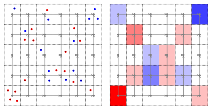
Below is shown two examples of a multi-point and the corresponding node based function . On the left, there is a collection of points with a weight of +1 denoted by red dots, and points with a weight of -1 denoted by blue dots. For each volume , the weights of all of the contained points are added together and the total weight is divided by to spread it out over the volume . On the right, shades of red denote positive values for , while shades of blue denote negative values for . White means that for the current node .
Multi point example on the left, and function on the right.
Multi point example on the left, and function on the right.
The example directed graph with the example multi-volume.
The discrete analog to volumes using a directed graph is that a volume is a collection of nodes: . The combined volume region denoted by is and the total volume amount is .
Volume can be denoted by a node based membership function: where for each node , it is the case that . The notation denotes with the parameter not shown.
A superposition of volumes forms a "multi-volume". Any node based function that returns real values can be the membership function of a multi-volume. For example, given the node based function can be expressed as the following superpositions:
is the superposition of volumes with the respective weights .
is the superposition of volumes with the respective weights .
It is important to note that given an arbitrary node based function, decomposing the multi-volume denoted by the function into a superposition of volumes is not unique, as shown above where a node based function is decomposed into multiple superpositions of volumes.
Any node based function that denotes a "potential" is best interpreted as a multi-volume.
The example directed graph with the example multi-path.
The discrete analog to paths using a directed graph is that a path is a series of edges and orientations: where is the edge and is an indicator that is if is traversed in the preferred direction, and is if is traversed in the opposite direction. The path must be unbroken: for each it must be that . The combined path denoted by is (path is path the orientation reversed) and the total length is .
A path can be denoted by the edge based function where for each edge , it is the case that where . The term arises from the fact that the path is "spread out" over the thickness of . The notation denotes with the parameter not shown.
A superposition of paths forms a "multi-path". Any edge based function that returns real values can denote a multi-path. For example, assuming that for all , the edge based function can be expressed as the following superpositions:
is the superposition of paths , and with the respective weights .
is the superposition of paths , and with the respective weights .
It is important to note that given an arbitrary edge based function, decomposing the multi-path denoted by the function into a superposition of paths is not unique, as shown above where an edge based function is decomposed into multiple superpositions of paths.
Any edge based function that denotes "flow density" (flow per unit cross-sectional area) is best interpreted as a multi-path.
Below is shown two examples of a multi-path and the corresponding edge based function . On the left a superposition of multiple paths is shown. For each surface , the total "flow" through is computed and is then divided by to spread it out over the surface . On the right, the flow enters a surface through the green side and leaves through the red side. The density of the flow is depicted by the strength of the shading. If the green to red orientation coincides with the orientation of , then is positive. If the green to red orientation is opposite the orientation of , then is negative.
Multi path example on the left, and edge based function on the right.
Multi path example on the left, and edge based function on the right.
The example directed graph with the example multi-surface.
The discrete analog to oriented surfaces using a directed graph is that an oriented surface is a collection of edges and orientations: where all of the edges are distinct and is an indicator that describes the surface's orientation. Each edge is an edge that passes through the surface, and is if passes through the surface in the preferred direction, and is if passes through the surface in the opposite direction. The combined surface denoted by is (surface is surface with the orientation reversed) and the total area is .
A surface can be denoted by the edge based function where for each edge , it is the case that . The term arises from the fact that the surface is "spread out" over the length of . The notation denotes with the parameter not shown.
A superposition of surfaces forms a "multi-surface". Any edge based function that returns real values can denote a multi-surface. For example, assuming that for all , the edge based function can be expressed as the following superpositions:
is the superposition of surfaces and with the respective weights .
is the superposition of surfaces and with the respective weights and .
It is important to note that given an arbitrary edge based function, decomposing the multi-surface denoted by the function into a superposition of surfaces is not unique, as shown above where an edge based function is decomposed into multiple superpositions of surfaces.
Any edge based function that denotes the "rate of gain" (rate of gain per unit length) is best interpreted as a multi-surface.
Below is shown two examples of a multi-surface and the corresponding edge based function . On the left a superposition of multiple surfaces is shown. For each curve , the net number of times edge penetrates in the preferred direction, referred to as the "gain" across , is computed and is then divided by to spread the gain out over the curve . On the right, the net gain is positive if an edge is traversed from the green end to the red end. The amount of gain is depicted by the strength of the shading. If the green to red orientation coincides with the orientation of , then is positive. If the green to red orientation is opposite the orientation of , then is negative.
Multi surface example on the left, and edge based function on the right.
Multi surface example on the left, and edge based function on the right.
A multi-volume and a multi-point is shown. The red volumes and points have a weight of +1, and the cyan volumes and points have a weight of -1. The intersection contributed by a point is its weight times the weight assigned to the volume that contains the point. The total intersection weight in this image is: N = (+1)x(+1+1+1-1-1) + 0x(+1+1-1-1-1) + (-1)x(+1-1) = +1.
Given an arbitrary point and volume , let denote an indicator function that returns 1 if point is contained by volume and returns 0 if otherwise.
Node based function denotes the point , and node based function denotes the volume .
The indicator function can be computed via the following sum:
.
The term cancels out the in .
counts the number of times point occurs in volume which can only be 0 or 1 for simple points and volumes. This count can be generalized to sets of points. Let denote a collection of points. The collection of points can be denoted by the node based function . The number of points from that are contained by volume can again be computed by the sum:
.
In the general case, given a node based function that denotes a multi-point, and a node based function that denotes a multi-volume, then the total weight of all the occurrences of being inside of is . The quantity is called the net intersection or the total intersection weight of with .
A path is shown intersecting a surface multiple times. The boundary of the surface has a counter-clockwise orientation. The net number of times that the surface is crossed in the preferred direction is +1-1+1+1+1 = 3.
Given an arbitrary path and surface , let denote the number of times path passes through surface in the preferred direction minus the number of times path passes through surface in the opposite direction. For an arbitrary , and an arbitrary , if then the link of path coincides with the segment of surface . If , then and passes through in the preferred direction. If , then and passes through in the opposite direction.
can be computed via the following sum:
. The term cancels out the from , and the term cancels out the from .
In the general case, given an edge based function that denotes a multi-path, and an edge based function that denotes a multi-surface, then the total weight of all the intersections of with is . The quantity is called the net intersection or the total intersection weight of with .
A directed graph that models the Cartesian coordinate system. One dimension is suppressed for simplicity.
The discrete model used for Cartesian coordinates will consist of an infinite 3 dimensional grid of nodes that spans . To establish the model, the following is needed:
A spacing for the x-coordinates.
A spacing for the y-coordinates.
A spacing for the z-coordinates.
For each triplet of integer indices , there exists a node and 3 edges , , and .
The origin and terminal nodes of are and
The origin and terminal nodes of are and
The origin and terminal nodes of are and
The Cartesian coordinate associated with node is , and the space associated with node is .
The volume of node is .
The length of edge is .
The length of edge is .
The length of edge is .
The area of edge is .
The area of edge is .
The area of edge is .
Given a scalar field over Cartesian coordinates, will be approximated by the node based function . Function is defined by for each .
Given a vector field over Cartesian coordinates, will be approximated by the edge based function . Function is defined by ; ; and .
A directed graph that models the cylindrical coordinate system. For simplicity, the vertical/z dimension is not shown.
The discrete model used for Cylindrical coordinates will consist of an infinite 3 dimensional cylindrical grid of nodes that spans . To establish the model, the following is needed:
A spacing for the coordinate .
A large positive integer that will yield a spacing for the coordinate .
A spacing for the coordinate .
Each node will correspond to a unique triplet of integers, and will be denoted by . The cylindrical coordinate denoted by will be .
Clearly, due to the nature of cylindrical coordinates (such as the fact that coordinate is cyclical), not every triplet will be allowed. The following three domains will be defined: , , and .
There exists a node for each .
There exists an edge for each such that and
There exists an edge for each such that and
There exists an edge for each such that and
Next, the volume of each node and the lengths and area of each edge will be calculated. To simplify notation, let for any nonnegative real number .
For each the cylindrical coordinate that corresponds to is , and the space (described using cylindrical coordinates) associated with is
For each the volume of node is
For each the length and area of edge is and respectively.
For each the length and area of edge is and respectively.
For each the length and area of edge is and respectively.
Given a scalar field over cylindrical coordinates, will be approximated by the node based function . Function is defined by for each .
Given a vector field over cylindrical coordinates, will be approximated by the edge based function . Function is defined by:
A directed graph that models the spherical coordinate system. The image is a cross-section that contains the vertical/z axis, which is "up" in the image.
The discrete model used for Spherical coordinates will consist of an infinite 3 dimensional spherical grid of nodes that spans . To establish the model, the following is needed:
A spacing for the coordinate .
A large positive integer that will yield a spacing for the coordinate .
A large positive integer that will yield a spacing for the coordinate .
Each node will correspond to a unique triplet of integers, and will be denoted by . The spherical coordinate denoted by will be .
Clearly, due to the nature of spherical coordinates (such as the fact that coordinate is cyclical), not every triplet will be allowed. The following three domains will be defined: , , , and .
There exists a node for each .
There exists an edge for each such that and
There exists an edge for each such that and
There exists an edge for each such that and
Next, the volume of each node and the lengths and area of each edge will be calculated. To simplify notation, let for any nonnegative real number , and let for any nonnegative real number and any real number .
For each the spherical coordinate that corresponds to is , and the space (described using spherical coordinates) associated with is
For each the volume of node is
For each the length and area of edge is and
respectively.
For each the length and area of edge is and respectively.
For each the length and area of edge is and respectively.
Given a scalar field over spherical coordinates, will be approximated by the node based function . Function is defined by for each .
Given a vector field over spherical coordinates, will be approximated by the edge based function . Function is defined by:
A curvilinear coordinate system is a coordinate system such as cylindrical or spherical coordinates where the position may not follow a straight line as one of the coordinates is changed. To model an arbitrary curvilinear coordinate system in 3 dimensional space, let the coordinates be denoted by .
To avoid unnecessary repetition, the following notation will be used:
Given any number , and subset , then denotes the triple
Given any two triples of numbers , then
Given any two triples of numbers , then
denotes an arbitrary curvilinear coordinate .
denotes an arbitrary triplet of differences in the coordinates .
Let denote the position given by coordinate .
For each , the rate of change in the position at coordinate with respect to is given by: .
It will be assumed that , , and are all mutually perpendicular, which is the case for Cartesian, cylindrical, and spherical coordinates.
In addition, for each , vector will also denote a unit length normalization of .
For the purposes of simplicity, it will be assumed that the coordinates can be any triple of real numbers. Singularities such as the z-axis in cylindrical and spherical coordinates will not be considered by this model. Since singularities are not considered, this model will be considerably simpler than the models given for cylindrical and spherical coordinates.
To model the curvilinear coordinate system, a lattice of nodes connected by directed edges will be established:
Start by choosing "resolutions" for each coordinate denoted by . The quantities should all be strictly positive, and ideally should be as small as possible.
For each triplet of integer indices , a node will be created at position .
For each and for each triplet of integer indices , there will exist edge such that and .
For each , the volume of node is
For each and , the length and area of edge are and respectively.
Any node for which should be deleted along with all connecting edges.
For any edge for which and , then nodes and should be fused into a single node, and edge should be discarded. For any edge for which and , then edge should be discarded. Either action may be pursued when .
Given a scalar field over the curvilinear coordinate system, will be approximated by the node based function . Function is defined by for each .
Given a vector field over the curvilinear coordinates, will be approximated by the edge based function . Function is defined by for each and for each .
Let denote an arbitrary volume. Given a node based function , the "volume integral" of over is (recall that is the volume of node , and is the volume of space represented by ).
If node based function is an approximation of a scalar field , where , then is an approximation of the volume integral .
Recall that can be described via the node based function . This allows the expression . If node based function denotes a multi-volume, then .
most often denotes a density function, and denotes the total "mass" contained by multi-volume . The equality means that if is interpreted as a multi-point, then the total "mass" contained by is the total intersection weight of with .
Let denote an arbitrary path. Given an edge based function , the "path integral" of along is (recall that is the length of edge , and is the curve represented by ).
If edge based function is an approximation of a vector field , where , then is an approximation of the path integral .
Recall that can be described via the edge based function . This allows the expression . If edge based function denotes a multi-path, then .
most often denotes a rate of gain function, and denotes the total "gain" caused by along multi-path . The equality means that if is interpreted as a multi-surface, then the total "gain" generated along is the total intersection weight of with .
Let denote an arbitrary surface. Given an edge based function , the "surface integral" of over is (recall that is the cross-sectional area of edge , and is the surface which separates and ).
If edge based function is an approximation of a vector field , where , then is an approximation of the surface integral .
Recall that can be described via the edge based function . This allows the expression . If edge based function denotes a multi-surface, then .
most often denotes a flow density function, and denotes the total "flow" through multi-surface . The equality means that if is interpreted as a multi-path, then the total "flow" through is the total intersection weight of with .
Given an arbitrary multi-volume denoted by node based function , the multi-surface which is the inwards oriented surface of the multi-volume is denoted by the edge based function . When traversing an arbitrary edge, the net number (positive - negative) of transitions through surfaces is the change in .
Consider an arbitrary volume . The inwards oriented surface of is a surface defined by and . Volume is denoted by the node based function . The inwards oriented surface is denoted by the edge based function:
More generally, if node based function denotes a multi-volume, then the edge based function is the inwards oriented multi-surface boundary of . One required property of the inwards oriented multi-surface boundary is that it must obey linearity: meaning that if multi-volumes and have inwards oriented multi-surface boundaries and respectively, then the inwards oriented multi-surface boundary of is . In addition, given an arbitrary coefficients , the inwards oriented multi-surface boundary of is . The definition satisfies this linearity condition.
Given a node based function , the "gradient" of is the edge based function . For all , . The gradient denotes both the inwards oriented surface when is treated as a multi-volume, and the rate of change in along each edge in the preferred direction when is treated as a potential. Note that the gradient satisfies linearity as described above.
Computing potential differences from the gradient[edit | edit source]
The path integral along path of the gradient of is the difference in between the endpoints. The value of at each node is shown, and along the path the value of is shown at each edge. (the edge orientations are not shown for simplicity)
Let be two nodes that are linked by edge . Let be reached from by traversing edge in the direction specified by orientation .
The difference in between and is:
When given an arbitrary path that begins at node and ends at node , the difference in between and can be computed by adding the differences along each edge:
The equation is referred to as the "gradient theorem".
The following sections will demonstrate that the gradient defined for node based functions is consistent with the gradient for scalar fields in . This consistency will be shown for Cartesian, cylindrical, and spherical coordinates.
The Gradient in Various Coordinate Systems[edit | edit source]
All of Cartesian, cylindrical, and spherical coordinate systems will be modeled using the discrete model of curvilinear coordinates. The same shorthand notation will be used.
Starting with an arbitrary scalar field , the node based function that approximates is for all .
For each and , the gradient along edge is:
Given an arbitrary coordinate , let index the node whose position is "closest" to .
The gradient of scalar field is a vector quantity with components that are multiples of the basis vectors . The coefficient of is the gradient of along edges that are parallel to , and similarly for and . The fact that , , and are of unit length and mutually orthogonal (perpendicular) is important.
The gradient of scalar field at can now be approximated by the following:
Applying the curvilinear coordinate model to Cartesian coordinates means that , , and . It is also the case that , , and . Applying the formula for the gradient that was derived from the discrete model of curvilinear coordinates gives:
which is consistent with the formula for the gradient derived for continuous functions over Cartesian coordinates.
Applying the curvilinear coordinate model to cylindrical coordinates means that , , and . It is also the case that , , and . Applying the formula for the gradient that was derived from the discrete model of curvilinear coordinates gives:
which is consistent with the formula for the gradient derived for continuous functions over cylindrical coordinates.
Applying the curvilinear coordinate model to spherical coordinates means that , , and . It is also the case that , , and . Applying the formula for the gradient that was derived from the discrete model of curvilinear coordinates gives:
which is consistent with the formula for the gradient derived for continuous functions over spherical coordinates.
When an edge based function is depicted as a superposition of paths, the divergence denotes the starting point density minus the end point density. In this image, the flow is depicted using the brown arrows along each edge. More arrows means more flow. The numbers indicate the total flow generation at each node, which is also the net starting point weight.
If the edge based function denotes the "flow density" across each edge, then for an arbitrary edge , the total flow across in the preferred direction is . For an arbitrary node , the total flow being generated at node is . The "flow generation density" or "divergence" at node is:
Using a similar argument, given a multi-path denoted by edge based function , then for an arbitrary edge , the total "path weight" that traverses in the preferred direction is (recall that is the path weight per unit thickness of ). The total "path weight" that is "left behind" at an arbitrary node is . The path weight that is left behind is the starting point weight minus the ending point weight, no matter how multi-path is decomposed into a superposition of paths. The starting point weight minus the ending point weight is the "net starting point weight". By diffusing the net starting point weight over the volume of node , the node based function that denotes the "net starting point" is derived. This is the divergence .
It is a relatively simple matter to show that for an a simple path that starts at node and ends at node , that due to the fact that only the end points of may have a non-zero starting point weight. is a node based function that denotes the superposition of the starting node of with the final node of with respective weights of and .
A depiction of the discrete analog of Gauss's divergence theorem. The rate () and direction of the flow along each edge is shown by the number and direction of the arrows, and each node is labeled with the rate of flow generation (). A net flow of -4 is flowing out from the highlighted boundary, and the total flow generation contributed by the nodes inside the boundary is also -4.
Let denote an arbitrary volume, and let denote the outwards oriented surface of .
The total flow generation inside is:
The total flow generated inside is the total outwards flow through : . This is the discrete analog to Gauss's Divergence Theorem.
Given an arbitrary multi-volume and a multi-path, the net intersection weight of the path's net starting point with the volume is equal to the net intersection weight of the path with the volume's outwards oriented surface. In this case the net intersection is 3.
Interpreting as a multi-path, and as the net starting point of , then Gauss's Divergence Theorem can be expressed as: . Due to the fact that is the outwards oriented surface of , it must be the case that , since is the inwards oriented surface of . This gives:
Replacing with a multi-volume gives the generalization:
This equation can be interpreted as follows: The total intersection of the net starting point of multi-path with multi-volume is the net intersection of with the outwards oriented surface of .
It should also be noted that the equation can be reformatted to read as:
When is a simple path that starts at node and ends at node , the above equation reduces to the gradient theorem:
The gradient theorem and Gauss's Divergence Theorem are therefore equivalent with the general form: .
The following sections will demonstrate that the divergence defined for edge based functions is consistent with the divergence for vector fields in . This consistency will be shown for Cartesian, cylindrical, and spherical coordinates.
The Divergence in Various Coordinate Systems[edit | edit source]
All of Cartesian, cylindrical, and spherical coordinate systems will be modeled using the discrete model of curvilinear coordinates. The same shorthand notation will be used.
Starting with an arbitrary vector field , the edge based function that approximates is for all and .
For each , the divergence at node is:
Given an arbitrary coordinate , let index the node whose position is "closest" to .
The divergence of vector field at can now be approximated by the following:
Applying the curvilinear coordinate model to Cartesian coordinates means that , , and . It is also the case that , , and . Applying the formula for the divergence that was derived from the discrete model of curvilinear coordinates to vector field gives:
which is consistent with the formula for the divergence derived for continuous vector fields over Cartesian coordinates.
The Divergence in Cylindrical Coordinates[edit | edit source]
Applying the curvilinear coordinate model to cylindrical coordinates means that , , and . It is also the case that , , and . Applying the formula for the divergence that was derived from the discrete model of curvilinear coordinates to vector field gives:
which is consistent with the formula for the divergence derived for continuous vector fields over cylindrical coordinates.
Applying the curvilinear coordinate model to spherical coordinates means that , , and . It is also the case that , , and . Applying the formula for the divergence that was derived from the discrete model of curvilinear coordinates to vector field gives:
which is consistent with the formula for the divergence derived for continuous vector fields over spherical coordinates.
Consider an arbitrary path that begins and finishes on the same node. is a closed loop, and the edge based function that denotes satisfies for all nodes . The divergence-free property of arises from the fact that closed loops have no starting or ending points and leave every node that they enter.
A divergence-free edge based function is a superposition of closed loops.A directed graph with a set of basis loops highlighted in different colors.
A multi-loop is a superposition of loops, and any edge-based function that denotes a multi-loop is divergence-free. Moreover, any edge-based function that is divergence free can be expressed as a superposition of closed loops and hence denotes a multi-loop.
Given an arbitrary graph , a set of "basis" loops can be formed such that every multi-loop can be expressed as a unique linear superposition of the basis loops. A set of basis loops provides a means of expressing an arbitrary multi-loop as a list of coefficients. Each coefficient is a weight that is assigned to each basis loop. When the basis loops are multiplied by their respective weights and added together, the multi-loop that is represented by the list of coefficients is retrieved.
The set of all edge based functions is a vector space with dimension , and each edge based function is a vector whose entries are the list of values assigned to each edge. The set of all multi-loops is a subspace of the set of all edge based functions, and each multi-loop can be interpreted as a vector that is a linear combination of the loops from a set of basis loops.
Three approaches for generating a set of basis loops for an arbitrary graph will now be given:
To start, the following definitions are required:
A path component of graph is an "island" of where any two nodes on the island can be linked by a continuous path, and any edge that is connected to a node in the path component is part of the same component and vice versa.
A bridge is an edge that when removed breaks its host path component into two path components.
An arc, also referred to as a simple path, is a path where with the exception of the start and end nodes does not visit or traverse the same node or edge more than once.
A simple loop is a closed loop that does visit a node or edge twice on the same cycle.
A tree is a graph where any two nodes can be linked by exactly one simple path.
A spanning tree is a sub-graph of a path component that is both a tree and which includes every node from .
Generating Basis Loops Approach 1:
A depiction of how approach 1 generates basis loops by repeatedly including arcs. The original loop is shown in red, and successive colors add each arc.
To start, all edges that are "bridges" should be removed. After all bridges have been removed, any nodes that are not connected to any edges and are themselves path components are themselves removed. Let denote the resultant path components of . Let the set of basis loops start out empty. Let denote the set of nodes visited by the loops from . Let denote the set of edges that are traversed by loops from .
The following steps are now repeated for each path component for each :
Start by choosing an arbitrary simple loop from . Add loop to . For as long as there are nodes or edges in that are not contained by or , find an arc that starts and ends at nodes from . With the exception of the starting and ending nodes, arc must not visit a node or edge from or . The end nodes of can be linked by a path through the nodes and edges from and to form a simple loop that is then added to .
The above process forms a set of basis loops for .
Let denote the number of path components of . As bridges and single nodes are removed from , the quantity remains constant. After all bridges and single nodes have been removed, path component yields basis loops where and are the number of nodes and edges from respectively. The total number of basis loops is therefore . The vector space of multi-loops has dimensions.
Generating Basis Loops Approach 2:
A depiction of how approach 2 generates basis loops by using a spanning tree. The solid edges are included in the spanning tree. Each dashed edge corresponds to a basis loop formed from the dashed edge and the unique path through the spanning tree.
Let denote the path components of graph . is the number of path components of . For each , let denote a "spanning tree" for path component . Each edge from that is not part of the spanning tree corresponds to a basis loop. This basis loop is formed from edge and the unique arc that connects the end points of through the spanning tree .
For path component , let and respectively denote the number of nodes and edges from . The spanning tree contains edges, so edges from are not part of the spanning tree, and hence correspond to basis loops. The total number of basis loops from is .
Generating Basis Loops Approach 3:
A third approach to generating a set of basis loops for graph proceeds by identifying the loops that pass through each node. To start, the set of nodes is ordered to form .
For each node , a set of basis loops is assigned to . These basis loops are confined to the nodes and are required to pass through . These loops will be chosen such that no nonzero linear superposition of these loops will result in an edge based function where all edges that connect to are assigned 0.
Each edge has 2 endings: and . With respect to node , let denote the set of all edge endings that connect to , excluding any edges that connect to nodes from . The set can now be partitioned into subsets according to the following equivalence relation: two edge endings belong to the same partition if and only if there exists a simple loop that is confined to the nodes and that visits node exactly once, arriving through or and leaving through the other ending. Let denote the partitioning of .
For each partition , choose an ending that will serve as the "prime ending". Each other ending from will correspond to a basis loop that leaves through and returns to through , never visiting any nodes from .
For each and , each ending from corresponds to exactly 1 basis loop. Each edge will contribute at most 1 ending to the total set , including edges that start and end on the same node. To count the number of basis loops, it is necessary to count the number of edges that do not contribute any endings to . These edges are the edges that contain a "prime ending" and do not begin and end on the same node.
To determine , let denote graph where the nodes and any connected edges have been removed. will denote the number of path components of . where is the number of path components of , and . Start with and reintroduce node and any connected edges to restore . Introducing creates a new path component. Connecting to a disconnected path component via an edge will reduce the number of path components by 1, but will also create an edge that contains a prime ending. Connecting to an already connected path component via an edge will not change the number of path components, nor create an edge with a prime ending. The number of prime endings that are connected to node not counting edges that start and end on is (the +1 compensates for the path component that introduces by default).
so the number of basis loops is which is in agreement with the other approaches.
Given an arbitrary oriented closed surface and an arbitrary oriented closed path, this image demonstrates how the number of times the path leaves the surface is equal to the number of times the path enters the surface.
Consider an arbitrary surface . Surface is "closed" if it has the following property: any path that is also closed must cross surface in the preferred direction and against the preferred direction an equal number of times. In mathematical terms, this means that given any closed path that .
Any conservative edge based function (denoted by arrows in this image) is the superposition of closed surfaces (denoted by the dashed lines).
An edge based function is "conservative" if any path integral of along an arbitrary closed path is 0: . In a similar manner to how any divergence free edge based function denotes a multi-loop, any conservative edge based function denotes a "multi-closed surface", which is the superposition of any number of closed surfaces.
An example of multiple surfaces sharing the same boundary.
A surface that is not closed is said to have a "boundary". Non-closed surfaces that share a common boundary can be grouped into "equivalence classes" and treated as though they are identical. It is relatively simple to observe that if surfaces and share a common boundary then the surface denoted by the edge based function is a closed surface since surfaces and form the two halves of a "clam shell" that when added form a closed surface ( is with the orientation reversed). The edge based function is therefore conservative. The difference between edge based functions that denote multi-surfaces with a common boundary denotes a multi-closed surface, and is hence conservative. If edge based function denotes an arbitrary multi-surface, then when given any conservative edge based function , the edge based function denotes a multi-surface with the same boundary as .
Given an arbitrary edge based function that denotes a multi-surface, will denote the boundary of , and will denote the set of all edge based functions that have the same boundary as . For any edge based function , if and only if . Moreover, if and only if is conservative.
Multi-surfaces, and their corresponding edge based functions, that all share a common boundary will be grouped into a single "equivalence class" and treated as if they are identical. An edge based function "represents" its equivalence class . An equivalence class effectively denotes the common boundary shared by all surfaces , and will be referred to as a "boundary".
The property of an edge based function being conservative is linear, which means that given conservative edge based functions and and coefficients and , it will be the case that the linear superposition is also conservative. The linearity of being conservative implies that: given edge based functions and where and , then for any coefficients . The previous property implies that the linear superposition of boundaries and can be performed unambiguously by choosing "representative" surfaces and and generating a surface that represents the linear superposition .
The set of all conservative edge based functions (the set of all closed surfaces) is a vector space, and the set of all equivalence classes/boundaries is a vector space.
A set of basis closed surfaces can be generated by the following simple process: Let denote the path components of . For each , a set of basis closed surfaces for path component can be produced by wrapping each node except for 1 in a basis surface as shown below. Any "bubble" can be generated by adding the bubbles that individually wrap each node inside the bubble. A surface that only wraps the remaining node can be generated by adding all of the bubbles that wrap the other nodes in the path component, and then reversing the orientation. The number of basis closed surfaces is where is the number of nodes from path component . The total number of basis closed surfaces for graph is .
A set of basis equivalence classes/boundaries can be generated by the following simple process: Let denote the path components of . For each , let denote a "spanning tree" for path component . Each edge from that is not part of the spanning tree corresponds to a basis equivalence class which consists of all edge based functions that can be formed by adding a conservative edge based function to the edge based function that is only at edge and for all other edges. The number of basis equivalence classes for path component is where and are the number of nodes and edges from path component respectively. is the number of edges from spanning tree . The total number of basis equivalence classes is . This is the same as the number of basis closed loops.
The fact that the previously mentioned set of basis of equivalence classes is in fact a basis, which means that every equivalence class is a unique linear superposition of the basis equivalence classes, can be confirmed by the following observations: Let be an arbitrary edge based function. A conservative edge based function can be created by letting for all edges that are in the spanning trees, and choosing values for at the edges that are not in the spanning trees such that is conservative. The difference is 0 for all edges in the spanning trees. The coefficients for each basis equivalence class are the values that attains at each non spanning tree edge. Moreover, any non-zero choice of coefficients for the basis equivalence classes will always create a non-conservative edge based function.
In the images below, the left image shows a set of basis closed surfaces, the middle image shows a set of basis non-closed surfaces, and the right image shows how any edge based function/surface (shown in blue) is the linear combination of basis non-closed surfaces plus a closed surface (shown in black).
A set of basis closed surfaces for the shown graph. Any closed surface is a linear combination of the basis surfaces. A surface that wraps the bottom right node can be formed by adding all of the shown basis surfaces, and then reversing the orientation.
A set of basis open surfaces for the shown graph. The edges in the spanning tree do not correspond to any basis surface. Any surface is a unique linear combination of the shown open surfaces plus a closed surface.
A non-closed surface, shown in blue, is the linear superposition of basis non-closed surfaces and a closed surface. Observe how the blue arrows on the edges are the sum of the black arrows (opposites cancel out).
The number of dimensions of the set of multi-loops is . The number of dimensions of the set of surface equivalence classes is also . This equivalence implies that it is possible to form a bijective (one to one and onto) linear mapping between the set of multi-loops and surface equivalence classes. In simpler terms, any multi-loop corresponds to a unique equivalence class of surfaces, and any equivalence class of surfaces corresponds to a unique multi-loop. The correspondence is linear, which means that given multi-loops and which respectively correspond to equivalence classes and , and coefficients and , then multi-loop corresponds to equivalence class .
Previously, when given a multi-surface denoted by edge based function , the boundary of was a hypothetical boundary assumed to be shared by all edge based functions whose difference with was a conservative edge based function. The boundary is now an edge based function that denotes the "counter-clockwise oriented boundary of ". Since the boundary of any surface is a loop, it will be required that is a multi-loop: . Mapping each surface to its boundary should also be linear: given surfaces and coefficients , then .
The bijective linear mapping between the set of multi-loops and surface equivalence classes maps each multi-loop to the equivalence class of surfaces which have as their common boundary.
A path is shown intersecting a surface multiple times. The boundary of the surface has a counter-clockwise orientation. The net number of times that the surface is crossed in the preferred direction is N = +1-1+1+1+1 = 3
Given path and surface , the net number of times that path intersects surface in the preferred direction is . This formula generalizes to edge based functions that denote multi-paths and multi-surfaces. Given edge based function that denotes a multi-path and edge based function that denotes a multi-surface, then the net number of times intersects in the preferred direction is .
It is also important to note that is linear with respect to and : and . It is also important to note that if is a multi-loop, and is a multi-closed surface (conservative), then . This latter property implies that given surfaces with a common boundary (), then since is conservative.
Two surfaces, each with a counter-clockwise oriented boundary, are shown. The net number of times each boundary intersects the other surface is the same. The red boundary passes through the green surface in the preferred direction 2 times, and the green boundary passes through the red surface in the preferred direction 2 times.
One requirement of the mapping of a boundary to each surface equivalence class is that given multi-surfaces and , the net number of times the counter clockwise oriented boundary passes through in the preferred direction is identical to the net number of times passes through in the preferred direction: . See the 2nd image on the right for an example of this property.
Since is linear with respect to and , and is linear with respect to , the condition is linear with respect to and :
Since the condition is linear, mapping each multi-loop to the surface equivalence class that have the multi-loop as their common boundary is done by determining a set of basis multi-loops and a set of basis surface equivalence classes such that for all , it is the case that . For each , corresponds to and the rest of the mapping is determined via linearity. Given an arbitrary multi-surface , expressing the equivalence class as a linear combination of basis surface equivalence classes: means that .
One such choice of basis multi-loops and basis surface equivalence classes can be determined as follows: Let denote the path components of . For each , let denote a "spanning tree" for path component . Each edge that is not part of any spanning tree corresponds to both a basis loop and a basis surface equivalence class. The basis loop is the loop that passes through edge and the unique path through a spanning tree that links the endpoints of . A surface that is part of the basis surface equivalence class is the surface that contains edge alone. It is easy to check that , and when given different edges and , that . This is only one example of a pair of a set of basis multi-loops and a set of basis surface equivalence classes (this example also does not make sense, as the prescribed boundary of each basis surface passes through the surface itself).
This example will demonstrate the duality of loops and surfaces using an example from electrical engineering: two simple circuits that are magnetically linked to themselves and to each other.
Three images describing the scenario are shown below:
The left image depicts a circuit diagram that denotes the circuits that are the subject of this example. Each loop consists of a voltage source in series with a resistor, and a self inductance followed by a mutual inductance. At the bottom of the image, the "magnetic circuit" is shown. The magnetic circuit carries magnetic flux instead of electric current, and helps to quantify the self and mutual inductance between the two loops of current.
The center image depicts the orientation of the magnetic circuit relative to the electric circuit. As can be seen, the magnetic flux through the first loop is measured relative to "down", while the magnetic flux through the second loop is measured relative to "up".
The right image depicts the directed graph that model the electric circuit. The set of nodes is and the set of edges is .
The origin and terminal nodes of each edge are: ; ; ; ; ; ; and .
There are 4 basis loops: ; ; ; and . These loops are the respective counterclockwise boundaries of the following 4 surfaces: ; ; ; and . It can be determined that the paths intersect the surfaces the following numbers of times:
Note that the above table is symmetric along its diagonal.
An electric and magnetic circuit that will be subject of this example.
The magnetic circuit is upright relative to the electric circuit. "Up" in the magnetic circuit protrudes from the page in the electric circuit.
A directed graph that will be used to model the electric and magnetic circuits, along with chosen basis loops and their corresponding surfaces.
The goal will be to derive expressions for the self inductances , and the mutual inductance .
An edge based function will denote the magnetic field density at each edge in the edge's preferred orientation.
A total current of flows around loop . This current flows outwards through surface , so due to Ampere's law, the total path integral of around is ( is the magnetic permeability of free space). Therefore:
A total current of flows around loop . This current flows outwards through surface , so due to Ampere's law, the total path integral of around is . Therefore:
The divergence of the magnetic field at any node is 0: . Therefore:
The following equations describe the magnetic field which is present in the magnetic circuit:
Solving the above equations yields:
The magnetic flux through the first loop (surface ) is:
The magnetic flux through the second loop (surface ) is:
This means that the self inductances of the first and second loop are respectively:
(the coefficient of in the expression for )
and
(the coefficient of in the expression for )
The mutual inductance is:
(the coefficient of in the expression for , or the coefficient of in the expression for )
Given an arbitrary edge based rate-of-gain function , and an arbitrary multi-loop (), the "circulation" of around is . With fixed, the circulation is a linear function of : .
A large loop can be decomposed into an ensemble of tiny loops.A large loop can be decomposed into an ensemble of tiny loops.
As seen in the images to the right, a large loop can be decomposed into a sum of smaller loops, and since the circulation is linear with respect to the loop that is being followed, the total circulation around the large loop is simply the sum of the circulations around the little loops.
Each edge is its own little surface: , and any surface is a linear combination of these basis surfaces. Any surface can be expressed as the following linear combination: . The length term cancels out the factor of in . If the circulation of around the counter clockwise boundary of each basis surface is computed, then the total circulation around the counter clockwise boundary of can be computed via the same linear combination:
The circulation per unit area of surface is . This "circulation density" at edge will be referred to as the "curl" and denoted by the edge based function .
The total circulation around the counter clockwise boundary of is . This is the discrete analog to Stokes' Theorem.
Computing the counter-clockwise boundary of a surface[edit | edit source]
The counter-clockwise boundary of the red surface is generated by the curl around each of the blue loops that wrap around the boundary.Given an oriented surface, a cross-section of which is shown here, the circulation around a tiny loop is only non-zero at the boundaries. The curl is oriented in the direction of the counter-clockwise boundary.
Let be an arbitrary multi-surface. Since can be expressed as the linear combination , the counterclockwise boundary is the linear combination of boundaries: .
Given arbitrary edges , it is the case that due to the requirement placed on the boundaries of surfaces. This restriction can also be expressed as: .
The linear combination that describes becomes:
The counterclockwise boundary of multi-surface is therefore the curl: .
Stoke's theorem becomes:
which is equivalent to:
which is an exact rephrasing of the condition .
All of Cartesian, cylindrical, and spherical coordinate systems will be modeled using the discrete model of curvilinear coordinates. The same shorthand notation will be used. However, the graph will be modified as follows:
Applying the curvilinear coordinate model to Cartesian coordinates means that , , and . It is also the case that , , and . Applying the formula for the curl that was derived from the discrete model of curvilinear coordinates to vector field gives:
Applying the curvilinear coordinate model to cylindrical coordinates means that , , and . It is also the case that , , and . Applying the formula for the curl that was derived from the discrete model of curvilinear coordinates to vector field gives:
Applying the curvilinear coordinate model to spherical coordinates means that , , and . It is also the case that , , and . Applying the formula for the curl that was derived from the discrete model of curvilinear coordinates to vector field gives:


![{\displaystyle [a,b]}](https://wikimedia.org/api/rest_v1/media/math/render/svg/9c4b788fc5c637e26ee98b45f89a5c08c85f7935)

![{\displaystyle [x_{0},x_{1}],[x_{1},x_{2}],...,[x_{N-1},x_{N}]}](https://wikimedia.org/api/rest_v1/media/math/render/svg/a7153a308a53d3f179be19e493bdc740ba6e6db2)


![{\displaystyle x_{i}^{*}\in [x_{i-1},x_{i}]}](https://wikimedia.org/api/rest_v1/media/math/render/svg/dafeab86f1179399f11208ee27a15c76434aed3d)


![{\displaystyle \max _{x\in [a,b]}|f(x,\Delta x)-g(x,\Delta x)|\to 0}](https://wikimedia.org/api/rest_v1/media/math/render/svg/227d4790e966eaddead5ad14495c0c5bc46981b5)
![{\displaystyle \max _{x\in [a,b]}{\frac {|f(x,\Delta x)-g(x,\Delta x)|}{\Delta x}}\to 0}](https://wikimedia.org/api/rest_v1/media/math/render/svg/e7d2e6e4cad984715da85fc0f8c0de7f7dc65b0e)


 Multi point example on the left, and function on the right.
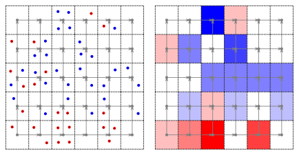 Multi point example on the left, and function on the right.


 Multi path example on the left, and edge based function on the right.
 Multi path example on the left, and edge based function on the right.


 Multi surface example on the left, and edge based function on the right.
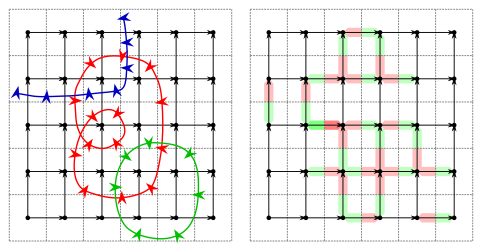 Multi surface example on the left, and edge based function on the right.


![{\displaystyle \omega _{3}(n_{(i,j,k)})=\left[i\Delta x-{\frac {\Delta x}{2}},i\Delta x+{\frac {\Delta x}{2}}\right]\times \left[j\Delta y-{\frac {\Delta y}{2}},j\Delta y+{\frac {\Delta y}{2}}\right]\times \left[k\Delta z-{\frac {\Delta z}{2}},k\Delta z+{\frac {\Delta z}{2}}\right]}](https://wikimedia.org/api/rest_v1/media/math/render/svg/d60cabe408721c39a5b2fba0cc3a88567b0cd22a)


![{\displaystyle \omega _{3}(n_{(i,j,k)})=\left\{{\begin{array}{cc}[(i-{\frac {1}{2}})\Delta \rho ,(i+{\frac {1}{2}})\Delta \rho ]\times [(j-{\frac {1}{2}})\Delta \phi ,(j+{\frac {1}{2}})\Delta \phi ]\times [(k-{\frac {1}{2}})\Delta z,(k+{\frac {1}{2}})\Delta z]&(i>0)\\{[0,{\frac {\Delta \rho }{2}}]}\times [0,2\pi ]\times [(k-{\frac {1}{2}})\Delta z,(k+{\frac {1}{2}})\Delta z]&(i=0)\\\end{array}}\right.}](https://wikimedia.org/api/rest_v1/media/math/render/svg/dca51828436233a68d9ce29a75168b4583ac9e03)


![{\displaystyle j_{\text{real}}\in [0,N_{\theta }]}](https://wikimedia.org/api/rest_v1/media/math/render/svg/fb70e94b8bb8f93d6118e80584005fc4f19a5e82)
![{\displaystyle \omega _{3}(n_{(i,j,k)})=\left\{{\begin{array}{cc}[(i-{\frac {1}{2}})\Delta r,(i+{\frac {1}{2}})\Delta r]\times [(j-{\frac {1}{2}})\Delta \theta ,(j+{\frac {1}{2}})\Delta \theta ]\times [(k-{\frac {1}{2}})\Delta \phi ,(k+{\frac {1}{2}})\Delta \phi ]&(i>0\;{\text{and}}\;0<j<N_{\theta })\\{[(i-{\frac {1}{2}})\Delta r,(i+{\frac {1}{2}})\Delta r]}\times [0,{\frac {\Delta \theta }{2}}]\times [0,2\pi ]&(i>0\;{\text{and}}\;j=0)\\{[(i-{\frac {1}{2}})\Delta r,(i+{\frac {1}{2}})\Delta r]}\times [\pi -{\frac {\Delta \theta }{2}},\pi ]\times [0,2\pi ]&(i>0\;{\text{and}}\;j=N_{\theta })\\{[0,{\frac {\Delta r}{2}}]}\times [0,\pi ]\times [0,2\pi ]&(i=0)\\\end{array}}\right.}](https://wikimedia.org/api/rest_v1/media/math/render/svg/77673c85705504f63b6ef77632c3d3a315eded56)


![{\displaystyle [k]_{C}}](https://wikimedia.org/api/rest_v1/media/math/render/svg/1595ef65d9d48d5c5b6e224304e0c8f732a47763)
![{\displaystyle [k]_{C}=\left(\left\{{\begin{array}{cc}k&(1\in C)\\0&(1\notin C)\end{array}}\right.,\left\{{\begin{array}{cc}k&(2\in C)\\0&(2\notin C)\end{array}}\right.,\left\{{\begin{array}{cc}k&(3\in C)\\0&(3\notin C)\end{array}}\right.\right)}](https://wikimedia.org/api/rest_v1/media/math/render/svg/dc5dbdd6edacf23ee05a0720f02c657b248fd499)


![{\displaystyle t^{\bullet }(e_{\xi _{c},I})=n_{I+[1]_{c}}}](https://wikimedia.org/api/rest_v1/media/math/render/svg/4c611fe8d491c6a0e84f2968b63e33861de1d9ae)


![{\displaystyle \tau _{1}(e_{\xi _{c},I})=\Delta \xi _{c}|\mathbf {u} _{\xi _{c}}((I+[0.5]_{c})\Delta \Xi )|}](https://wikimedia.org/api/rest_v1/media/math/render/svg/b67126d5863d2579342eea26e0cd7ab33bb85abc)
![{\displaystyle \tau _{2}(e_{\xi _{c},I})=\prod _{c'\neq c}\Delta \xi _{c'}|\mathbf {u} _{\xi _{c'}}((I+[0.5]_{c})\Delta \Xi )|}](https://wikimedia.org/api/rest_v1/media/math/render/svg/12e698360ecc6b95cebb0628880284a6b7e93e99)


![{\displaystyle F_{\text{approx}}(e_{\xi _{c},I})=F_{\xi _{c}}((I+[0.5]_{c})\Delta \Xi )}](https://wikimedia.org/api/rest_v1/media/math/render/svg/ebd847ee39a5433143a41a9951086a09742396d3)


![{\displaystyle ={\frac {f_{\text{approx}}(n_{I+[1]_{c}})-f_{\text{approx}}(n_{I})}{\Delta \xi _{c}|\mathbf {u} _{\xi _{c}}(I\Delta \Xi )|}}}](https://wikimedia.org/api/rest_v1/media/math/render/svg/cd70330f4a31a30ebcc652a30c8f409f70d8f0e8)
![{\displaystyle ={\frac {f(I\Delta \Xi +[\Delta \xi _{c}]_{c})-f(I\Delta \Xi )}{\Delta \xi _{c}|\mathbf {u} _{\xi _{c}}((I+[0.5]_{c})\Delta \Xi )|}}}](https://wikimedia.org/api/rest_v1/media/math/render/svg/da3d3e96a22f09ac19cd6482c021e911a97931c0)


![{\displaystyle =\sum _{c=1}^{3}{\frac {f(I(\Xi )\Delta \Xi +[\Delta \xi _{c}]_{c})-f(I(\Xi )\Delta \Xi )}{\Delta \xi _{c}|\mathbf {u} _{\xi _{c}}((I(\Xi )+[0.5]_{c})\Delta \Xi )|}}\mathbf {v} _{\xi _{c}}(I(\Xi )\Delta \Xi )}](https://wikimedia.org/api/rest_v1/media/math/render/svg/188b76e036f61632e3c9baeff486f19f3e3079e0)
![{\displaystyle \approx \sum _{c=1}^{3}{\frac {f(\Xi +[\Delta \xi _{c}]_{c})-f(\Xi )}{\Delta \xi _{c}|\mathbf {u} _{\xi _{c}}(\Xi )|}}\mathbf {v} _{\xi _{c}}(\Xi )}](https://wikimedia.org/api/rest_v1/media/math/render/svg/07857585a258227b57988cd0936c7deda2556891)


![{\displaystyle ={\frac {1}{\prod _{c=1}^{3}\Delta \xi _{c}|\mathbf {u} _{\xi _{c}}(I\Delta \Xi )|}}\sum _{c=1}^{3}(\tau _{2}(e_{\xi _{c},I})F_{\text{approx}}(e_{\xi _{c},I})-\tau _{2}(e_{\xi _{c},I-[1]_{c}})F_{\text{approx}}(e_{\xi _{c},I-[1]_{c}}))}](https://wikimedia.org/api/rest_v1/media/math/render/svg/c149b65a5883aae9c4b092f002fd0149af913dbd)
![{\displaystyle ={\frac {1}{\prod _{c=1}^{3}\Delta \xi _{c}|\mathbf {u} _{\xi _{c}}(I\Delta \Xi )|}}\sum _{c=1}^{3}\left((\prod _{c'\neq c}\Delta \xi _{c'}|\mathbf {u} _{\xi _{c'}}(I\Delta \Xi +[0.5\Delta \xi _{c}]_{c})|)F_{\xi _{c}}(I\Delta \Xi +[0.5\Delta \xi _{c}]_{c})-(\prod _{c'\neq c}\Delta \xi _{c'}|\mathbf {u} _{\xi _{c'}}(I\Delta \Xi -[0.5\Delta \xi _{c}]_{c})|)F_{\xi _{c}}(I\Delta \Xi -[0.5\Delta \xi _{c}]_{c})\right)}](https://wikimedia.org/api/rest_v1/media/math/render/svg/5accc3e521f5db57feb515b5d34ac6c039274dbf)

![{\displaystyle ={\frac {1}{\prod _{c=1}^{3}\Delta \xi _{c}|\mathbf {u} _{\xi _{c}}(I(\Xi )\Delta \Xi )|}}\sum _{c=1}^{3}{\bigg (}(\prod _{c'\neq c}\Delta \xi _{c'}|\mathbf {u} _{\xi _{c'}}(I(\Xi )\Delta \Xi +[0.5\Delta \xi _{c}]_{c})|)F_{\xi _{c}}(I(\Xi )\Delta \Xi +[0.5\Delta \xi _{c}]_{c})}](https://wikimedia.org/api/rest_v1/media/math/render/svg/05f78a878cb9893c0e758f11b43bdca6a1763960)
![{\displaystyle -(\prod _{c'\neq c}\Delta \xi _{c'}|\mathbf {u} _{\xi _{c'}}(I(\Xi )\Delta \Xi -[0.5\Delta \xi _{c}]_{c})|)F_{\xi _{c}}(I(\Xi )\Delta \Xi -[0.5\Delta \xi _{c}]_{c}){\bigg )}}](https://wikimedia.org/api/rest_v1/media/math/render/svg/a1d50fe76b9f6fa57cfc6fa2e93b53ff65eee952)
![{\displaystyle \approx {\frac {1}{\prod _{c=1}^{3}\Delta \xi _{c}|\mathbf {u} _{\xi _{c}}(\Xi )|}}\sum _{c=1}^{3}\left((\prod _{c'\neq c}\Delta \xi _{c'}|\mathbf {u} _{\xi _{c'}}(\Xi +[0.5\Delta \xi _{c}]_{c})|)F_{\xi _{c}}(\Xi +[0.5\Delta \xi _{c}]_{c})-(\prod _{c'\neq c}\Delta \xi _{c'}|\mathbf {u} _{\xi _{c'}}(\Xi -[0.5\Delta \xi _{c}]_{c})|)F_{\xi _{c}}(\Xi -[0.5\Delta \xi _{c}]_{c})\right)}](https://wikimedia.org/api/rest_v1/media/math/render/svg/f676464bc6f3fb76c400cddd7262b2356253543b)
![{\displaystyle ={\frac {1}{\prod _{c=1}^{3}|\mathbf {u} _{\xi _{c}}(\Xi )|}}\sum _{c=1}^{3}{\frac {1}{\Delta \xi _{c}}}\left((\prod _{c'\neq c}|\mathbf {u} _{\xi _{c'}}(\Xi +[0.5\Delta \xi _{c}]_{c})|)F_{\xi _{c}}(\Xi +[0.5\Delta \xi _{c}]_{c})-(\prod _{c'\neq c}|\mathbf {u} _{\xi _{c'}}(\Xi -[0.5\Delta \xi _{c}]_{c})|)F_{\xi _{c}}(\Xi -[0.5\Delta \xi _{c}]_{c})\right)}](https://wikimedia.org/api/rest_v1/media/math/render/svg/1b76366fc167067c309c7f27e74896a07e06204e)


![{\displaystyle {\mathfrak {B}}[f]}](https://wikimedia.org/api/rest_v1/media/math/render/svg/8783f2b11a6380327c80b1b5a248c5ce38e49833)

![{\displaystyle g\in {\mathfrak {B}}[f]}](https://wikimedia.org/api/rest_v1/media/math/render/svg/ae4a133a18a3f7dfb46296a37b6d497afee668e9)


 A set of basis closed surfaces for the shown graph. Any closed surface is a linear combination of the basis surfaces. A surface that wraps the bottom right node can be formed by adding all of the shown basis surfaces, and then reversing the orientation.
 A set of basis open surfaces for the shown graph. The edges in the spanning tree do not correspond to any basis surface. Any surface is a unique linear combination of the shown open surfaces plus a closed surface.
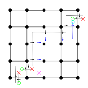 A non-closed surface, shown in blue, is the linear superposition of basis non-closed surfaces and a closed surface. Observe how the blue arrows on the edges are the sum of the black arrows (opposites cancel out).


![{\displaystyle \{{\mathfrak {B}}[g_{1}],{\mathfrak {B}}[g_{2}],...,{\mathfrak {B}}[g_{|{\mathcal {E}}|-|{\mathcal {N}}|+H}]\}}](https://wikimedia.org/api/rest_v1/media/math/render/svg/cc19563a5ed2b1545ad8d85b73d163126900166c)


![{\displaystyle {\mathfrak {B}}[g_{i}]}](https://wikimedia.org/api/rest_v1/media/math/render/svg/94f8777accfe94776b460aeba5abee330729794d)

![{\displaystyle {\mathfrak {B}}[g]}](https://wikimedia.org/api/rest_v1/media/math/render/svg/a0158ff1879fcf5668dec6af66681c4d42e78705)
![{\displaystyle {\mathfrak {B}}[g]=\sum _{i=1}^{|{\mathcal {E}}|-|{\mathcal {V}}|+H}c_{i}{\mathfrak {B}}[g_{i}]}](https://wikimedia.org/api/rest_v1/media/math/render/svg/8949276d703c4ed4e505dd4da4af54a4bbe3ecda)


![{\displaystyle \tau _{2}(e_{\xi _{c},I})=\prod _{c'\neq c}(\Delta \xi _{c'}|\mathbf {u} _{\xi _{c'}}((I+[0.5]_{c})\Delta \Xi )|)}](https://wikimedia.org/api/rest_v1/media/math/render/svg/378b485aefeb92a9aa4de302727abfd5218f601e)


![{\displaystyle \langle (e_{\xi _{c+1},I+[0.5]_{c}-[0.5]_{c+1}-[0.5]_{c+2}},+1),(e_{\xi _{c+2},I+[0.5]_{c}+[0.5]_{c+1}-[0.5]_{c+2}},+1),(e_{\xi _{c+1},I+[0.5]_{c}-[0.5]_{c+1}+[0.5]_{c+2}},-1),(e_{\xi _{c+2},I+[0.5]_{c}-[0.5]_{c+1}-[0.5]_{c+2}},-1)\rangle }](https://wikimedia.org/api/rest_v1/media/math/render/svg/ff4d0a4f54c4eb4938949575c8284b7447cd71cf)
![{\displaystyle n_{I+[0.5]_{c}-[0.5]_{c+1}-[0.5]_{c+2}};n_{I+[0.5]_{c}+[0.5]_{c+1}-[0.5]_{c+2}};n_{I+[0.5]_{c}+[0.5]_{c+1}+[0.5]_{c+2}};n_{I+[0.5]_{c}-[0.5]_{c+1}+[0.5]_{c+2}}}](https://wikimedia.org/api/rest_v1/media/math/render/svg/b76f1a4527b27d2a08e0e1cda4a4336700468fef)


![{\displaystyle F_{\text{approx}}(e_{\xi _{c+1},I+[0.5]_{c}-[0.5]_{c+1}-[0.5]_{c+2}})\tau _{1}(e_{\xi _{c+1},I+[0.5]_{c}-[0.5]_{c+1}-[0.5]_{c+2}})}](https://wikimedia.org/api/rest_v1/media/math/render/svg/7a2431dbb1ad9eaf6b0bd0cd00fd1e00eeda6151)
![{\displaystyle +F_{\text{approx}}(e_{\xi _{c+2},I+[0.5]_{c}+[0.5]_{c+1}-[0.5]_{c+2}})\tau _{1}(e_{\xi _{c+2},I+[0.5]_{c}+[0.5]_{c+1}-[0.5]_{c+2}})}](https://wikimedia.org/api/rest_v1/media/math/render/svg/e3c84fa1895f95a577a9e5f3c06bcbea1ffb8a85)
![{\displaystyle -F_{\text{approx}}(e_{\xi _{c+1},I+[0.5]_{c}-[0.5]_{c+1}+[0.5]_{c+2}})\tau _{1}(e_{\xi _{c+1},I+[0.5]_{c}-[0.5]_{c+1}+[0.5]_{c+2}})}](https://wikimedia.org/api/rest_v1/media/math/render/svg/e56a2d4448b6006df78d6b7bcf44b5553d49cee6)
![{\displaystyle -F_{\text{approx}}(e_{\xi _{c+2},I+[0.5]_{c}-[0.5]_{c+1}-[0.5]_{c+2}})\tau _{1}(e_{\xi _{c+2},I+[0.5]_{c}-[0.5]_{c+1}-[0.5]_{c+2}}){\bigg )}}](https://wikimedia.org/api/rest_v1/media/math/render/svg/e541bbebc88b9092354547f45f47528460f7fa1a)
![{\displaystyle ={\frac {1}{|\mathbf {u} _{\xi _{c+1}}((I+[0.5]_{c})\Delta \Xi )||\mathbf {u} _{\xi _{c+2}}((I+[0.5]_{c})\Delta \Xi )|\Delta \xi _{c+1}\Delta \xi _{c+2}}}{\bigg (}}](https://wikimedia.org/api/rest_v1/media/math/render/svg/a0b9c1ba2e2f34b5979f7b6045c300c91142f8c8)
![{\displaystyle F_{\xi _{c+1}}((I+[0.5]_{c})\Delta \Xi -[0.5\Delta \xi _{c+2}]_{c+2})|\mathbf {u} _{\xi _{c+1}}((I+[0.5]_{c})\Delta \Xi -[0.5\Delta \xi _{c+2}]_{c+2})|\Delta \xi _{c+1}}](https://wikimedia.org/api/rest_v1/media/math/render/svg/112f9074370c0df472caf60f1a43e38264fe3abe)
![{\displaystyle +F_{\xi _{c+2}}((I+[0.5]_{c})\Delta \Xi +[0.5\Delta \xi _{c+1}]_{c+1})|\mathbf {u} _{\xi _{c+2}}((I+[0.5]_{c})\Delta \Xi +[0.5\Delta \xi _{c+1}]_{c+1})|\Delta \xi _{c+2}}](https://wikimedia.org/api/rest_v1/media/math/render/svg/fa8b25b8fe28d7ac9f66d4a9c61a0dcdb2ec7c8e)
![{\displaystyle -F_{\xi _{c+1}}((I+[0.5]_{c})\Delta \Xi +[0.5\Delta \xi _{c+2}]_{c+2})|\mathbf {u} _{\xi _{c+1}}((I+[0.5]_{c})\Delta \Xi +[0.5\Delta \xi _{c+2}]_{c+2})|\Delta \xi _{c+1}}](https://wikimedia.org/api/rest_v1/media/math/render/svg/a613d316f943aff9047e9a1860def541f86df6ae)
![{\displaystyle -F_{\xi _{c+2}}((I+[0.5]_{c})\Delta \Xi -[0.5\Delta \xi _{c+1}]_{c+1})|\mathbf {u} _{\xi _{c+2}}((I+[0.5]_{c})\Delta \Xi -[0.5\Delta \xi _{c+1}]_{c+1})|\Delta \xi _{c+2}}](https://wikimedia.org/api/rest_v1/media/math/render/svg/b11245a33d26f3d22913f3bc887d3b9a5348c879)


![{\displaystyle (I+[0.5]_{c})\Delta \Xi }](https://wikimedia.org/api/rest_v1/media/math/render/svg/31be0fc1f2da99d0001f602ffd3c3770ad44e3a5)

![{\displaystyle F_{\xi _{c+1}}(\Xi -[0.5\Delta \xi _{c+2}]_{c+2})|\mathbf {u} _{\xi _{c+1}}(\Xi -[0.5\Delta \xi _{c+2}]_{c+2})|\Delta \xi _{c+1}}](https://wikimedia.org/api/rest_v1/media/math/render/svg/a8bfdcf6821f13dad41a57845e6dd8d1c8799a68)
![{\displaystyle +F_{\xi _{c+2}}(\Xi +[0.5\Delta \xi _{c+1}]_{c+1})|\mathbf {u} _{\xi _{c+2}}(\Xi +[0.5\Delta \xi _{c+1}]_{c+1})|\Delta \xi _{c+2}}](https://wikimedia.org/api/rest_v1/media/math/render/svg/589ef44809e226f870183b991d141111cf4b130c)
![{\displaystyle -F_{\xi _{c+1}}(\Xi +[0.5\Delta \xi _{c+2}]_{c+2})|\mathbf {u} _{\xi _{c+1}}(\Xi +[0.5\Delta \xi _{c+2}]_{c+2})|\Delta \xi _{c+1}}](https://wikimedia.org/api/rest_v1/media/math/render/svg/218da4eebfaa7ab52cccd5fafa78b8c5f0cd9c0c)
![{\displaystyle -F_{\xi _{c+2}}(\Xi -[0.5\Delta \xi _{c+1}]_{c+1})|\mathbf {u} _{\xi _{c+2}}(\Xi -[0.5\Delta \xi _{c+1}]_{c+1})|\Delta \xi _{c+2}}](https://wikimedia.org/api/rest_v1/media/math/render/svg/51e079eae7cfa3954133f0c7760f9945fdc861d8)


![{\displaystyle {\frac {1}{\Delta \xi _{c+1}}}(F_{\xi _{c+2}}(\Xi +[0.5\Delta \xi _{c+1}]_{c+1})|\mathbf {u} _{\xi _{c+2}}(\Xi +[0.5\Delta \xi _{c+1}]_{c+1})|-F_{\xi _{c+2}}(\Xi -[0.5\Delta \xi _{c+1}]_{c+1})|\mathbf {u} _{\xi _{c+2}}(\Xi -[0.5\Delta \xi _{c+1}]_{c+1})|)}](https://wikimedia.org/api/rest_v1/media/math/render/svg/9e8c97090b880fc48bf303a9a54d9387dd5fbdd5)
![{\displaystyle -{\frac {1}{\Delta \xi _{c+2}}}(F_{\xi _{c+1}}(\Xi +[0.5\Delta \xi _{c+2}]_{c+2})|\mathbf {u} _{\xi _{c+1}}(\Xi +[0.5\Delta \xi _{c+2}]_{c+2})|-F_{\xi _{c+1}}(\Xi -[0.5\Delta \xi _{c+2}]_{c+2})|\mathbf {u} _{\xi _{c+1}}(\Xi -[0.5\Delta \xi _{c+2}]_{c+2})|)}](https://wikimedia.org/api/rest_v1/media/math/render/svg/13fb6e10035a7915c7b2aca7d348dbb7f0de0cae)


