Trigonometry/For Enthusiasts/Lissajous Figures
Lissajous Curve
[edit | edit source].jpg)
A Lissajous curve is the graph of the equations:

with chosen values of and and with varying.


This is a generalisation of the graph we drew of the circle in the exercise plotting cos t vs sin t.
In fact we get that circle if we put
- and


in the Lissajous curve equation.
|
Check this
|
This family of curves was investigated by Nathaniel Bowditch in 1815, and later in more detail by Jules Antoine Lissajous in 1857.
Examples
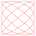
[edit | edit source]Below are examples of Lissajous figures, all with δ = 0.
-
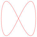 a = 1, b = 2 (1:2)
 -
 a = 3, b = 2 (3:2)
 -
 a = 3, b = 4 (3:4)
 -
 a = 5, b = 4 (5:4)
 -
 a = 5, b = 6 (5:6)
 -
 a = 9, b = 8 (9:8)


The appearance of the figure is highly sensitive to the ratio a/b. For a ratio of 1, the figure is an ellipse, with special cases including circles (A = B, δ = π/2 radians) and lines (δ = 0). Another simple Lissajous figure is the parabola (a/b = 2, δ = π/2). If δ = 0, the curve must pass through the origin, since in that case when t = 0 both x and y are 0. Very different curves may arise from the same value of a/b but different values of δ.
|
Check this
|
Other ratios produce more complicated curves, which are closed only if a/b is rational. The visual form of these curves is often suggestive of a three-dimensional knot, and indeed many kinds of knots, including those known as Lissajous knots, project to the plane as Lissajous figures.
Lissajous figures where a = 1, b = N (N is a natural number) and

are Chebyshev polynomials of the first kind of degree N.
Generation
[edit | edit source]Prior to modern computer graphics, Lissajous curves were typically generated using an oscilloscope (as illustrated). Two phase-shifted sinusoid inputs are applied to the oscilloscope in X-Y mode and the phase relationship between the signals is presented as a Lissajous figure.
On an oscilloscope, we suppose x is CH1 and y is CH2, A is amplitude of CH1 and B is amplitude of CH2, a is frequency of CH1 and b is frequency of CH2, so a/b is a ratio of frequency of two channels, finally, δ is the phase shift of CH1.
Application for the case of a = b
[edit | edit source]When the input to an LTI system is sinusoidal, the output is sinusoidal with the same frequency, but it may have a different amplitude and some phase shift. Using an oscilloscope that can plot one signal against another (as opposed to one signal against time) to plot the output of an LTI system against the input to the LTI system produces an ellipse that is a Lissajous figure for the special case of a = b. The eccentricity of the resulting ellipse is a function of the phase shift between the input and output, with an eccentricity of 1 corresponding to a phase shift of and an eccentricity of corresponding to a phase shift of 0 or 180 degrees. The figure below summarizes how the Lissajous figure changes over different phase shifts. The arrows show the direction of rotation of the Lissajous figure.


Lissajous figures were first mentioned by Nathaniel Bowditch in 1815, and rediscovered by Jules Antoine Lissajous in 1857. If the periods are equal, the curve is always an ellipse. If one period is twice the other, we get a quartic curve; a special case is the lemniscate of Bernouilli.