Transportation Geography and Network Science/Network growth models
Background
[edit | edit source]Christaller (1933) examines the formation of central places according to the economic principle of traffic, stating, “the demand of the population, the cost of transportation, the cost of invested capital, etc., decisively influence the formation of a traffic system”. Transportation networks and land use are interdependent shapers of urban form. First, changes in land use alter travel demand patterns. Second, increased traffic drives officials to respond by expanding transportation facilities. Third, new transportation facilities change the accessibility pattern, which drives the location of activities and travel behavior.
Life-cycle Models
[edit | edit source]The life-cycle model predicts the share of deployment of a technology at a particular point in time.

Where:
= fractional share of technology (technology’s share of final market share)
= time
= model parameters


The literature on transportation network growth is not vast. Several researchers have considered the problem of modeling the structure of the network. Taaffe, et al. (1963) look at how roads emerge from a port in a developing country, Garrison and Marble (1965) consider the order in which links were constructed in Irish railroads, Helbing et al. (1997) adopt the active walker model of Lam and Pochy (1993) allowing walkers moving on a landscape to change it, Watts and Strogatz. (1998) propose a small worlds model and Barabasi et al. (1999a,b) suggest preferential attachment so that already connected nodes get more connections, which explains hubbing, while Yamins et al. (2003) co-evolve roads with urban settlements.
Empirical Models
[edit | edit source]A line of research estimating empirical models of the expansion of existing transportation facilities and the construction of new links has also been undertaken (Levinson and Karamalaputi 2003a, b).
Agent-based Models
[edit | edit source]Several papers developed an agent-based model (using link-agents) to treat the organization, growth, and contraction of network elements with fixed or random land use patterns (Yerra and Levinson 2004, Levinson and Yerra 2005). These models have been extended in a series of papers (collected in Xie and Levinson 2011), relaxing assumptions of fixed network topology, fully decentralized agents, and lack of congestion.
System of Network Growth (SONG) model
[edit | edit source]The SONG model can be accessed at [1]

Overview
[edit | edit source]The components of the System of Network Growth (SONG) model include travel demand, revenue, cost, and investment. The travel demand model converts population and employment data into traffic using the given network topology and determines the link flows by following the traditional planning steps of trip generation, trip distribution, and traffic assignment (for simplicity, a single mode is assumed). A revenue model determines the price the traffic must pay for using the road depending on speed, flow and length of the link. In the experiments below, link length is fixed, and so revenue is independent of link length, however that assumption, like all assumptions in the model, can be relaxed. A cost model calculates the cost required to maintain link speeds depending on traffic flow. Revenue in excess of maintenance costs will be invested on the link to improve its condition using an investment model until all revenue is consumed. After upgrading (or downgrading) each link in the network, the time period is incremented and the whole process is repeated until an equilibrium is reached or it is clear that it cannot be achieved. An overview and inter-connection of these models is shown in Figure 1.
Complex systems consist of numerous autonomous agents, the interaction of which results in system properties different from agent properties (the speed of an individual link cannot tell you of the existence of a road, a single road does not of itself indicate the existence of a hierarchy of roads (with distinct freeways, signalized arterials, local streets). A hierarchy describes the scale of particular network elements compared to other elements of the same type. Modeling a transportation network as a complex system involves modeling nodes (which act both as intersections and what in conventional travel demand literature would be considered traffic zone centroids), links (road sections), land use cells, and traveler properties and their interactions. In SONG, network topology is taken as a given, and link and system properties are modeled as a function of alternative inputs.
SONG models network evolution as a bottom-up, rather than a top-down process. Planners and engineers would argue that transportation network investments are decisions that are now driven, or coordinated, by centralized organizations such as state departments of transportation or metropolitan planning organizations that make major investment decisions using a forecasting model and planning process to test and evaluate alternative scenarios. Local jurisdictions, of which there are many in some metropolitan areas, make investments on lower level roads. Certainly these organizations do affect new investment, but the decision to build or expand a link is also constrained by many facts on the ground, actual traffic on the link, competing parallel links, and complementary and upstream and downstream links, the costs of expansion, and limited budgets. If we can generate convincing representations of network structure without any centralized planning or direction, perhaps planning is not as important in shaping urban areas as it is sometimes given credit for, and instead is following demand in a relatively simple way.
The examples here use a grid network structure for several reasons. First, the examples presented test alternative land use patterns; simultaneously altering both the network topology and the land use makes drawing conclusions about effects more difficult. Second, the grid is a widely used topology that can be found throughout most of the United States, (particularly the Midwest and West since the Land Ordinance of 1785 established the Public Land Survey System) where the basic structure of the grid was laid out before more detailed factors like the width of streets (and thus their importance), and the associated land uses were determined. Third, the grid is not limited to the United States, it has been used in various forms in a variety of places, among them Giza in Egypt, Mohenjo-daro in the Indus Valley, Babylon in the time of Hammurabi, various capital cities in China and other Asian countries, the Greek cities designed by Hippodamus such as Miletus, most Roman city planning, Teotihuancan in Mexico, and Spanish colonies throughout the Americas. Certainly other network topologies (or the absence of topology) are possible to test, and are left as an exercise for the student.
Land Use and Trip Generation
[edit | edit source]Land use is modeled as a grid arrangement of land blocks called land use cells. Each land use cell stores its location, population density and market density (an aggregation of retail and office space). Using this data a trip generation model calculates trips attracted and produced from each land use cell. In order to keep the analysis simple it is assumed that trips produced from a land use cell are directly proportional to population density and trips attracted to a land use cell are directly proportional to market density. Therefore the information that a land use cell holds can be considered trips generated.
Let be the ordered pair that represent the location of land use cell, with being the position of the cell in the x-direction, being position of the cell in the y-direction. Let and represent total number of land use cells in the and direction respectively. Let and be the trips produced from and trips attracted to land use cell respectively. Since the total number of trips produced in a geographical area equals the total number of trips attracted, the following equation always holds true.


Each land use cell is assigned to the closest network node. The cost of commuting between a land use cell and its nearest network node is neglected. The total trips produced and attracted from a network node by summing up trips of all the land use cells assigned to that network node. Let be the set of all the land use cells that are closer to network node than to any other network node. The nearest network node to a land use cell is assigned by comparing the distances between the land use cell and network nodes around it. The trips at each network node are simply the trips of all the cells allocated to it.


Where,
is trips produced from (originating at) network node ,


is trips attracted to (destined for) network node .


Network Layer
[edit | edit source]Any network can be considered as a collection of nodes (or vertices) that are connected by links (or edges or arcs). The transportation network here is a directed graph . Let denote sequentially numbered nodes and set denote sequentially numbered directed links that connects nodes in . Let denote the number of elements (number of nodes) in set and denote the number of elements (number of links (or arcs)) in set . Let denote a set of origin nodes and denote a set of destination nodes. Note that in the networks modeled herein, i.e. each node acts as both origin and destination. A link connected from origin node to destination node is represented as .


Let and represent the and coordinates of node in Cartesian coordinates. Let be the length of the link . Then and are static variables of a node and is the static property of a link . Let be the average speed of a vehicle on link at time step and is referred as link speed. Travel time on the link, which is the ratio of link length to link speed, is the impedance to flow. It is assumed that there is no impedance to the flow at a network node. Since the links in the graph are directional – i.e. a link from node 1 to 2 differs from a link from 2 to 1 – we have a directed graph.


Trip Distribution Models
[edit | edit source]Trip distribution assigns trips generated at an origin to a destination, resulting in an origin-destination matrix (OD matrix), where rows sum to origin trips by zone and columns to destination trips.
Let be the number of trips generated from network node and ending at network node in time step . Then the following relationships hold at every time step .


The singly constrained gravity model is adopted in this research (Hutchinson, 1974). The number of trips in each OD pair is:

where the negative exponential model is used:

such that

where: is dummy variable equal to 1 if link belongs to the shortest path between and , 0 otherwise.

is the generalized cost of commuting on arc

is the generalized cost of commuting between nodes and .

To define the generalized cost of commuting between any two nodes, it is necessary to define the generalized cost of commuting on a link. The generalized cost of commuting on a link in time step is assumed to consist of two parts; travel time converted to monetary value and a toll, which is allowed to vary depending on link length and speed.

where:
is the generalized cost of commuting on arc

is a base toll (the fixed cost of using a link of unit length and speed)

is a coefficient representing the pricing structure with link length: the elasticity of tolls with respect to length

is a coefficient representing the pricing structure with link speed: the elasticity of tolls with respect to speed

Route Assignment
[edit | edit source]Using the OD matrix and the shortest path information computed using Dijkstra’s Algorithm (Chachra et al., 1979), flow on each link can be calculated by summing the trips between any origin and destination that passes through that link.

where, is the traffic flow on the link in time step .

Revenue Model
[edit | edit source]The revenue model estimates how much revenue is collected, where revenue is simply the product of the toll and the flow. The toll itself is a generalized function described in equation of above, which varies with length and speed. The revenue () is the money available for each link in year .


where: is a model parameter to annualize flow.

Cost Model
[edit | edit source]Cost of highway maintenance and expansion is often found to be well-represented by the Cobb-Douglas form in empirical models (e.g. Levinson and Gillen 1998 and Levinson and Yerra 2002, which both found better fits with the Cobb-Douglas model than other functional forms). The costs are typically a function of output (e.g. flow by vehicle type), network size, prices, and a measure of quality. This model does not consider prices (which are assumed to be exogenous and fixed over time (or rising at the same rate as incomes)), but does consider the other three variables. The cost of maintaining the links in a given year is given by


where:
is the (annual) unit cost of maintenance for a link,

are coefficients indicating economies or diseconomies of scale with respect to length, flow, speed respectively.

Investment Model
[edit | edit source]In the proposed investment model, if a link-agent has excess revenue in a given year (beyond what is required to maintain the link at its current speed), it can use the revenue for improving the link (making it faster). If a link runs a deficit, it cannot afford full maintenance, and the link speed deteriorates. An equation reflecting this is given by:

In the literature, there are to date no empirical investment models to go by, so there is some arbitrariness to this function. The investment model is admittedly simple and myopic, which we believe is a strength of the model if it can reproduce results that are thought to be generated by much more complicated processes. Future research can test alternative investment models, including the use of centralized agents like governments or banks to redirect the investment of excess funds, or to ensure that basic levels of service are provided even if the link is unprofitable.
An averaging rule is applied to ensure links and their opposites share the same design, which is typical of roadways.

This condition need not be applied in cases where symmetric conditions from the traffic assignment model are applied, as those symmetric conditions automatically ensure that and have same flows.

Experiments
[edit | edit source]Three land use patterns are considered: random, uniform, and bell shaped. Each of these categories is elaborated in the following sub-sections.
Randomly Distributed Land Use
[edit | edit source]The spatial distribution of land use properties like population and employment depends on many factors and some of these variables are interdependent. In randomly distributed land use, trips produced and trips attracted are each randomly distributed for each land use cell in the geography. The trips produced and attracted are distributed between given minimum and maximum values:

Uniform Land Use
[edit | edit source]A uniform land use pattern in which every cell throughout the geography has identical properties can be assigned by using the distribution shown in equation (14) by using identical and values. This kind of land use pattern is required to control the effect of land use on formation of hierarchies of roads.


Bell Shaped Land Use
[edit | edit source]
In reality the distribution of land use is not completely random. The distribution of land use variables in an urban area with a central business district can often be represented as bell or inverted bell shaped surfaces. In such a case the trips attracted are modeled to increase as the center of the geography is approached along a radial. Trips produced, which are proportional to residential density, are assumed to be at a minimum at the center, resembling an inverted bell shaped surface. The schematic representation of a cross-section of assumed distributions of trips produced and trips attracted along a radial direction are shown in Figure 2. The spatial distribution of trips attracted function is as shown in the equation:

where, is the position of the land use cell at the center of the downtown along x-axis,

is the position of the land use cell at the center of the downtown along y-axis, is a factor that depends on the spread of the downtown.


Substituting from the equation above into the initial equation gives:

Assuming an inverted bell shaped surface for trips produced, the distribution for is calculated using

where,

Model Parameters
[edit | edit source]Table 1 gives the values value of parameters in the model. These have been fixed where noted to allow comparability on the variables of interest in this study (land use patterns). The initial speed is assigned a unit value, and land use (number of trips produced and attracted per cell) is 10 units in the base scenario. The coefficient of the trip distribution model () in the land use experiments is taken to be 0.01, except where otherwise noted; a higher coefficient would imply travelers are more sensitive to travel costs, and thus make shorter trips, which are tested separately. Tolls are set to be increase linearly with link length and to be insensitive to road quality (speed). The revenue and cost coefficients are scaled to assume that every one of 365 days is equal, to annualize values (this is clearly an idealization that ignores, e.g., weekends). Costs increase linearly with length. There are economies of scale however, so as flow increases by 1%, costs increase by only 0.75%. Similarly as speed increases by 1%, cost only increases by 0.75%. This general assumption of economies of scale is supported by the literature, though the exact magnitude is debated. Small, Winston, and Evans (1989) reported significant economies of scale associated with pavement thickness, which represents its ability to handle loads. They also found evidence that there are slight economies of scale in the provision of road capacity; i.e. the capacity to handle traffic. Yerra and Levinson (2002) also report economies of scale for cars and trucks. These parameters are again fixed to allow us to explore the variables of interest.

| Variable | Description | ' | Base assumption |
| Initial Speed (integer) | 1 | ||
| Land use properties of cell z | 10 | ||
| Coefficient in Trip Distribution Model (land use experiments) | 0.01 | ||
| Coefficient in Revenue Model | 1.0 | ||
| Length power in Revenue Model | 1.0 | ||
| Speed power in Revenue Model | 0.0 | ||
| Tax rate in Revenue Model | 1.0 | ||
| Revenue Model parameter | 365 | ||
| μ | Unit cost in Cost Model | 365 | |
| Length power in Cost Model | 1.0 | ||
| Flow power in Cost Model | 0.75 | ||
| Speed power in Cost Model | 0.75 | ||


Results
[edit | edit source]Land Use Experiments
[edit | edit source]-
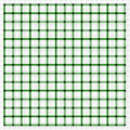 Base Case: Uniform Initial Speeds and Land use (U/U) - Spatial distribution of uniform speed for the initial network
 -
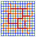
 Base Case: Uniform Initial Speeds and Land use (U/U) - Spatial distribution of speed for the network at equilibrium reached after 8 iterations.
 -
 Uniform initial speeds and random initial land use (U/R) -Spatial distribution of speed for experiment U/R after reaching equilibrium
 -
 Random initial speeds and random initial land use (R/R) - Spatial distribution of initial speed for experiment R/R (random initial speeds and random initial land use)
 -
 Random initial speeds and random initial land use (R/R) - Spatial distribution of speeds for the network after reaching equilibrium; The color and thickness of the link shows its relative speed or flow.
 -
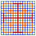
 Uniform initial speeds and bell-shaped initial land use (U/B) - Spatial distribution of final speeds for experiment U/B (uniform initial speeds and bell shaped land use)


The land use results presented are shown in Figures 3-7. Figure 3 presents the base case, with uniform initial network and uniform initial land use (denoted (U/U)). In the base case, an undifferentiated network evolves to a highly differentiated one, with both a major north-south and east-west axis, and two ring roads. The other figures are similar to the base case in that there is a hierarchy, but differ as the hierarchy is not so regular or symmetric. Those cases begin identically to the base case except for the treatment of initial speeds and land use characteristics. In the experiments with random land use, land use characteristics of the cells are randomly distributed between 10 and 15 trips. In this case, trips produced and trips attracted from a land use cell need not be the same though total trips produced and trips attracted by all land use cells are same. Link speeds in this model are dealt with in two ways; firstly (experiment U/R), speeds are assumed to be same for each link with magnitude 1, as in the base case. Secondly (experiment R/R), speeds are randomly distributed between 1 and 5. Typical solutions are shown in Figures 4 and 5.
Notice the similarity of resulting networks of experiments U/R and R/R. We believe the differences in land use distribution (and speeds) and the boundaries are responsible for the hierarchies in this case.
Figures 6 (U/B) and 7 (R/B) employ an urban bell-shaped land use distribution. Urban land use is distributed such that the network center coincides with the centers of the cup-shaped trips attracted and trips produced functions. Since more trips are attracted to the center of the network, it is natural to expect the links that lead to the center carry high traffic. Notice the uniform spacing of major roads in both the X and Y directions in Figure 6 and also the major roads are leading towards the center of the network where much of the activity lies. In Figure 6 there are three rings around the center, in contrast with Figure 3 that had only two major rings. Further, the major north-south and east-west axes divide, with some traffic diverted to the ring road, and other traffic proceeding through the center. Figure 7, with random initial speeds, has a similar pattern to Figures 4 or 5, with a single asymmetric ring around the center, though it is offset as the random initial conditions lead to different resulting networks. Spatial Interaction Experiments
Spatial Interaction Parameter Experiments
[edit | edit source]-
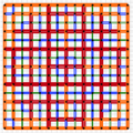
 Gravity model parameter variations with uniform network and land use (U/U) Spatial distribution of relative speeds at equilibrium for (top) (less sensitive to travel cost)
 -
 Gravity model parameter variations with uniform network and land use (U/U) Spatial distribution of relative speeds at equilibrium for (more sensitive to travel cost).
 -
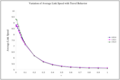 Variation of average link speed with w for 10X10, 11X11 and 15X15 networks.


In another experiment the coefficient in the friction factor () that represents travel behavior is tested for its sensitivity and the results are compared. In these experiments, the network and land use are both uniform with the base assumptions, so this is a variation of (U/U). If w is zero, trip distribution is independent of the cost of traveling. A higher (lower) value of w represents a society in which shorter (longer) trips are more frequent. The equilibrium spatial distribution of speeds for two w values that represent societies that prefer short-trips and long-trips are compared in Figure 8. As expected the spatial distribution of speeds for larger is much flatter with more relatively high-speed links than communities with a preference for long-trips, which are more hierarchical. However note, that while communities with a preference for short trips have more relatively high-speed links, they do not have more absolutely high-speed links, that is, their average link speed is lower than the community with a preference for long trips.
The variation of average traffic flow and speed with respect to the coefficient w for a few network sizes is as shown in Figures 9 and 10. As w increases the average traffic flow (speed) on the network drops as expected, indicating that societies where trips are longer produce more transportation revenue, and thus produce a better transportation infrastructure.
Conclusions
[edit | edit source]This analysis tested the effects three different types of land use (random, uniform, and bell-shaped) on a grid network. Each land use produced a different resulting hierarchy of roads, some producing more significant belt-roads, others a flatter network pattern. An experiment which varied the friction factor in the trip distribution (spatial interaction) model should that this parameter highly influences the spatial distribution of roads. We might observe that sometimes it is advantageous to have a flatter hierarchical distribution of link flows especially in cases where congestion (an externality of the system) is a problem, or where there are concerns about the reliability of vulnerable links. All of the scenarios lead us to conclude that the hierarchy of roads is an emergent property of transportation networks interacting with users. This finding occurred under very simple revenue, cost, and investment assumptions. The emergence of roads suggests networks are capable of self-organization.
Can self-organizing networks be planned? The difficulty of planning arises because the long-term morphological dynamics of transportation networks have long been unpredictable in nature due to the lack of proper forecasting tools, and they depend on many exogenous social, economical, political, and technological changes. We observe that in many ways cities are self-organizing, and the recent literature on fractal cities (Batty and Longley 1994) would support that point. Individual investment decisions that differ from a “market” equilibrium will shape the future evolution of the market or network. Clearly cities are both self-organizing and planned. Networks can be as well. Models such as the ones developed in this paper allow us to model the effects of planning decisions and decision-rules on the future morphology of networks. When combined with land use models, complete models of urban systems can be generated, allowing us to more fully understand what drives urban issues like congestion and sprawl. These tools enable the exploration of these problems, and possible solutions, in models, which should be more cost-effective in the long-run than running real-world experiments on functioning cities, which generally is infeasible. It is posited that agent-based network dynamics modeled according to principles of complex systems similar to the one presented in this research might prove to be useful.
For instance, in reality the land use distribution is neither uniform nor a perfect bell shaped surface. It is a very bumpy terrain with discontinuities and only certain small areas showing trends. The methods presented here provide the flexibility to use realistic land use patterns (e.g. Zhang and Levinson 2004), which provide more evidence of the utility of the model framework, but have the disadvantage of having multiple simultaneous aspects that cannot be disentangled as easily as with artificial networks and land use patterns.
In the face of self-organizing networks some mechanism is required to eliminate negative externalities. The points of intervention with travelers are well known (e.g. properly pricing travel), but the intervention with agents that build the network has to date been left to politics. There are rules those agents used (highly simplified here), that lead agencies to expand links, these rules are often made based on limited criteria (e.g. expand when average daily traffic exceeds X and pavement condition is poor). Better understanding these rules, and how they play out over time in a systems dynamics framework, gives us another way to reduce the negative effects associated with transportation.
As mentioned earlier the relationship between land use and transportation network dynamics is crucial. Many of the current urban problems are due to congestion and sprawl, which are byproducts of (or the solution to) imbalances between land use and travel demand and transportation infrastructure supply. Although the model presented in this paper does not explicitly consider the effects of networks on land use, it is speculated that modeling this feedback relationship will help planning transportation projects that supply the necessary infrastructure to manage congestion and sprawl. Moreover such models can be effective tools for both urban and transportation planners. Most of the traditional transportation planning models considers land use as a given variable (as in this model) but by including the dynamics of land use richer transportation as well as urban dynamics can be captured.
References
[edit | edit source]- Barabasi A, Albert R 1999 “Emergence of scaling in random networks.” Science 286 509-512
- Barabasi A, Albert R, Jeong H 1999 “Scale-free characteristics of random networks: the topology of the world wide web” Physica A 272 173-187
- Batty M, Longley P 1994 Fractal Cities (Academic Press, London)
- Chachra V, Ghare P, and Moore J 1979 Applications of Graph Theory Algorithms. (North Holland, New York)
- Christaller W 1933 Central Places in Southern Germany (Fischer, Jena, Germany) (English translation by Baskin, C (Prentice Hall, London 1966)).
- Fujita M, Krugman P, Venables, A 1999. The Spatial Economy: Cities, Regions, and International Trade (MIT Press, Cambridge, MA)
- Garrison W, Marble, D 1965 A Prolegomenon to the Forecasting of Transportation Development. United States Army Aviation Material Labs Technical Report (Office of Technical Services, United States Department of Commerce, Washington, DC)
- Helbing D, Keltsch J, Molnár P 1997 “Modeling the evolution of human trail systems” Nature 388: 47.
- Hutchinson B 1974 Principles of Urban Transportation Systems Planning. (McGraw-Hill, New York)
- Lam L, Pochy R 1993 “Active-walker models: growth and form in non-equilibrium systems” Computation simulation 7, 534.
- Lam L 1995 “Active walker models for complex systems” Chaos, Solitons and Fractals 6, 267-285.
- Levinson, D and Gillen, D 1998, “The Full Cost of Intericty Highway Transportation” Transportation Research part D 3:4 207-223,
- Levinson D and Karamalaputi R 2003a “Predicting the construction of new highway links” Journal of Transportation and Statistics 6(2/3) 81–89
- Levinson D and Karamalaputi R 2003b, “Induced supply: a model of highway network expansion at the microscopic level” Journal of Transport Economics and Policy, 37(3) 297–318
- Levinson, D and Yerra, B. 2002 “Highway Costs and the Efficient Mix of State and Local Funds” Transportation Research Record: Journal of the Transportation Research Board 1812 27-36
- Levinson D and Yerra B 2005 “Self Organization of Surface Transportation Networks” Transportation Science (in press)
- Lösch A 1954 The Economics of Location (Yale University Press, New Haven)
- Schweitzer F, Schimansky-Geier L 1994 “Clustering of active walkers in a two-component system” Physica A 206 359-379
- Small, K, Winston, C & Evans, C 1989 Road Work: A New Highway Investment Policy. Washington, DC: Brookings Institute.
- Taaffe E, Morrill R, Gould P 1963 “Transport expansion in underdeveloped countries: a comparative analysis.” Geographical Review 53 (4) 503-529
- Watts D, Strogatz S 1998 “Collective dynamics of ‘small-world’ networks”, Nature 393: 440-442.
- Yamins D, Rasmussen S, Fogel, D 2003 “Growing urban roads” Networks and Spatial Economics 3 69-85
- Yerra B, Levinson D 2004 “The emergence of hierarchy in transportation networks” Annals of Regional Science (in press).
- Xie, F., Levinson D 2011 Evolving Transportation Networks, Springer.
- Zhang L, Levinson D 2004 “A model of the rise and fall of roads” paper presented at the MIT Engineering Systems Symposium, March 2004, Cambridge, MA; copy available from Levinson, Department of Civil Engineering, University of Minnesota, Minneapolis