Strategy for Information Markets/Network Externalities/Demand Structure with Network Externalities
Graphs are a useful tool for exploring economics, so we want to be able to use them in studying markets with network externalities. However, the simple graphs of downward-sloping demand which get us so far in many markets are misleading when studying a market with strong demand-side economies of scale. Here, we're going to figure out what demand would look like in such a market, so we can use the graphs to answer questions later.
Influence of expected quantity
[edit | edit source] |
| Figure 1: Actual quantity demanded (Q) at $50 given expected quantity (QX) |
Start with the basic idea of network externalities: when more people consume a product, that product becomes more valuable to others. If we want to show this on a graph, we need to think carefully about exactly what we're showing, and what we want to leave off. To begin with, we'll leave off price. Price is important, so we'll leave it off by holding it constant, say at p = $50. Now, that $50 is important, but it will be the same for everything on the graph so we can ceteris paribus ignore it for the time being.
What should go on the graph? We're concerned with how many people want to purchase the product, but how many people want to purchase it depends on how many people purchase it. Graphing quantity versus itself doesn't seem likely to be productive, but we can make a tweak and get somewhere with it. Rather than graphing quantity versus quantity, we'll graph expected quantity versus quantity demanded.
Figure 1 shows a typical demand for a good with strong network externalities. The expected quantity (Qx) is on the horizontal axis, and the actual quantity demanded (Q) is on the vertical axis. Q is given as a function of Qx and of price, but price is being held constant. Notice some things about the shape of the curve:
- When expected quantity is low, actual quantity demanded is zero. This isn't always true in products with network externalities, but often can be. Nobody wants to pay $50 for a telephone if there's nobody else on the network they're interested in talking to. We'll consider this a typical case, and look at exceptions later.
- Quantity demanded is increasing. The curve for quantity demanded is sloping upwards. As more people join the network, more people want to join the network.
- Quantity demanded is increasing at a decreasing rate. A bigger network is always better[1], but it doesn't keep getting better as fast. When 20 people have a telephone, a new person joining the network is a big deal that increases the value of the network a lot. When 2 billion people have a telephone, one more person joining the network doesn't noticeably change the value for most telephone users. Since the value of the network doesn't change very much, it doesn't influence many more people to demand the product.
Demand equilibrium
[edit | edit source] |
| Figure 2: Equilibrium quantity demanded at a fixed price. |
We see a complete curve of possible quantities at the given price, but not all of those quantities are reasonable, at least not in the long run. We need to think about the relationship between expectations and the actual quantity demanded. Suppose that the actual quantity demanded is greater than the expected quantity. Then more will be purchased and expectations will change to more closely match the reality. What if the actual quantity demanded is lower than the expected quantity? Eventually, consumers will notice that few people are purchasing the product and expectations will lower to match the reality.
We're concerned with these demand equilibrium points--the quantities where the expectations match the reality, and so expectations have no reason to change.
We can find these points graphically by overlaying a 45-degree line on the graph. In Figure 2, along the 45-degree line Q = Qx, but the line doesn't show demand equilibria itself because it may be that the actual amount that will be demanded is less or more. To identify the demand equilibria, look at where the 45-degree line intersects the demand curve. At these intersection points expectations don't need to change because they are correct and the actual quantity demanded for those expectations are the same as the expectations. Each of those overlapping spots is a demand equilibrium.
In Figure 2, with this kind of strong network externalities, there are 3 demand equilibria. These are labeled (L) for "Low", (H) for "High", and (C), which will be explained shortly. We now want to think more precisely about how the market might move if it's not at one of those equilibria.
- Figure 3: Market response to being out of demand equilibrium
-
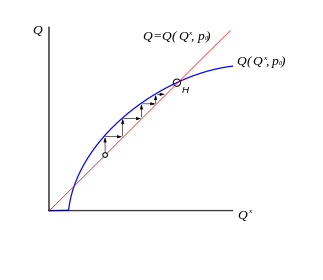 Figure 3(a)
 -
 Figure 3(b)
 -
 Figure 3(c)


Figure 3 shows three situations where the quantities are not at a demand equilibrium.
- In Figure 3(a), at the initial expectations, consumers will demand more. So the first arrow shows an increase in the quantity demanded. Expectations then need to catch up with this reality, so the second arrow shows expectations increasing until they reach the 45-degree line again where Q = Qx. At this expected quantity, a greater quantity is demanded, and so the third arrow shows the quantity demanded increasing again, and so forth toward demand equilibrium (H).
- In Figure 3 (b), at the initial expectations, consumers will demand less. So the first arrow shows a decrease in the quantity demanded. Expectations then catch up by falling, so the second arrow shows expectations decreasing until they reach the 45-degree line, and so forth toward demand equilibrium (H).
- In Figure 3 (c), just as in 3 (b), at the initial expectations, consumers will demand less. Quantity demanded and expectations decrease toward demand equilibrium (L).
 |
| Figure 4: General response to being out of demand equilibrium. |
Figure 4 gives a shorthand in arrows for the dynamics shown in Figure 3. Overall, if expectations are below (C), the market will move to demand equilibrium (L). If expectations are above (C), the market will move to demand equilibrium (H) (whether the market is originally between (C) and (H) or is greater than (H)).
Points (L), (C) and (H) are all demand equilibria, but (C) has a different character. It's an unstable equilibrium. A small shift away from (C) on the low side will send the market toward (L) and a small shift away on the high side will send the market toward (H). We'll refer to (c) as the critical mass for the market. If the market can achieve the critical mass, then it should go to the high-quantity demand equilibrium, but if it falls short of the critical mass, it will fall to the low-quantity demand equilibrium (likely with quantity demanded being zero).
Finding the demand curve
[edit | edit source] |
| Figure 5: Constructing a demand curve for a product with network externalities. |
In the previous section we found demand equilibria, but those are only equilibria for a specific price. We want to be able to use demand curves as we usually do in economic analysis. Figure 5 shows how we can use the demand equilibria to find the demand curve.
Instead of a single price, we choose 3 different prices: p1, p2 and p3, with p3 > p2 > p1. When the price goes up, the quantity-demanded curve goes down, because--at any given expected quantity--people aren't willing to buy as much. This is shown on the top graph as three curves for each of the three prices.
For each of the prices, we find the three demand equilibria: the (L), (C) and (H). The (L) in this example is always zero. It's marked with three points at p1, p2 and p3. The high demand has three levels for the three different prices, H1 at price p1, H2 at p2 and H3 at p3. We find those levels by finding the (H) demand equilibrium for each of the three prices, and tracing it down from the top graph to the bottom demand graph. As you'd expect on any typical demand graph, higher prices give you lower quantities demanded and this part of the demand curve slopes downward.
We similarly trace the critical mass for each of the three prices, and this gives us something different looking. The critical masses are marked as C1, C2 and C3. Rather than sloping down, the demand curve slopes up for the critical mass. At first that might seem to violate our economic intution, but recall it's the critical mass. We don't actually expect demand to ever be there. Instead, it's the dividing line between a network which will take off to (H) and one which will collapse to (L). This is indicated by drawing that portion of the demand curve with a dotted line--it's part of the demand structure which we don't want to forget, but we shouldn't look at it to see what quantity will be purchased at any particular price. This portion of the demand curve slopes up because as the price rises, it's harder to convince people to join the network. The higher price turns them off of the network, but if a lot of other people are in the network, that compensates for the higher price.
Using the demand curve
[edit | edit source] |
| Figure 5: Demand curve for a product with network externalities. |
We will usually not look at the Qx-vs-Q curves, and rely on demand curves such as the one derived in Figure 4. Figure 5 shows such a demand curve standing alone, with a particular price p.[2] At the price p, we can see three demand equilibria. (C) is the critical mass at price p, so we don't expect that quantity to be demanded. (L) and (H) are two probable quantities which might be demanded at price p.
Besides reading the two possible quantities demanded off the demand curve, we'll need to give thought to expectations, since what consumers expect to occur can influence which of those quantities are actually realized.
Shifts in demand
[edit | edit source]Similar to a demand curve for a typical good, if something happens to make the network good more attractive (possibly a technology improvement), the demand curve shifts up. If something happens to make it less attractive, the demand curve shifts down. When such shifts occur, they likely will leave the (L) "low" part of the curve unchanged.
Consumer surplus
[edit | edit source]A demand curve for a good with network externalities shows marginal willingness-to-pay for each potential quantity sold. In this way it is like a typical demand curve. However, because the demand curve for the product with network externalities shows demand equilibria, the meaning is a little different. This difference is significant enough that reading consumer surplus off the demand curve becomes impossible.
It may help to consider a discrete example. We'll consider 6 possible consumers of a product with network externalities. Suppose each of them values the good even without network externalities, and that they all get the same benefit from network externalities, with the benefit equal Q, the size of the network.
Their values without network externalities are 7, 5, 7, 3, 7, and 1. We'll follow the traditional idea for constructing a demand schedule or "curve" (although since it's discrete it's not really a curve in this case), and order the consumers from those who value the good most highly to those who value it least. Then we can plot their WTP on a graph.
| Consumer | Value w/o network externalities | Q | Value including Q |
|---|---|---|---|
| 1 | 7 | 1 | 7+1 = 8 |
| 2 | 7 | 2 | 7+2 = 9 |
| 3 | 7 | 3 | 7+3 = 10 |
| 4 | 5 | 4 | 5+4 = 9 |
| 5 | 3 | 5 | 3+5 = 8 |
| 6 | 1 | 6 | 1+6 = 7 |

The graph shows the value (WTP) for each of the six consumers. If we could read willingness-to-pay from this graph in the same way as a typical demand graph (which we can't), we could see that at a price of 6, the first consumer has a surplus of 8-6, the second of 9-6, etc. Adding up the differences for all the consumers, we would find a consumer surplus of 15.
This is wrong, though. The actual consumer surplus (which we can figure out from our original description, but not from the graph) is 30. The reason can be figured out from the first consumer. Their value for the good is 7+Q, where Q is the number of other people purchasing the good. When we draw the demand curve, each point on the curve was a demand equilibrium, so that expected quantity demanded and actual quantity demanded match. This is useful for drawing the demand curve, but it means the willingness-to-pay is only correct for that exact quantity.
| Q | WTP |
|---|---|
| 1 | 7+1 = 8 |
| 2 | 7+2 = 9 |
| 3 | 7+3 = 10 |
| 4 | 7+4 = 11 |
| 5 | 7+5 = 12 |
| 6 | 7+6 = 13 |
This table shows the willingness-to-pay for the good depending on how many people actually purchased it. If the price was 6, and all 6 consumers decided to purchase the good, the WTP of the first consumer would be 13, instead of the 8 shown on the graph.

The green areas on the updated graph show the WTP if every consumer assumes that 6 people will be purchasing the product. Now we can find the consumer surplus by summing the difference between consumer's values and the price they pay. However, this is only correct if 6 consumers actually purchase the product. If fewer or more purchased the product, this would also give an incorrect consumer surplus value.
Efficiency in competitive equilibrium
[edit | edit source]If a product has no externalities, we generally find that the competitive equilibrium is efficient. There are a number of ways economists talk about this. One was is to point out that, in a competitive equilibrium, the marginal willingness-to-pay (from the demand curve) is the same as the marginal cost. Since usually the marginal willingness-to-pay (WTP) is falling and/or the marginal cost is rising with increasing quantity, this means that ...
- ... selling any less than the competitive equilibrium is inefficient, because at lower quantities the marginal willingness-to-pay is higher than the marginal cost, and
- ... selling any more than the competitive equilibrium is inefficient, because at higher quantities the marginal willingness-to-pay is lower than the marginal cost.
The part of that which remains true with (positive) network externalities is that in competitive equilibrium, the marginal willingness-to-pay equals the marginal cost. The part which is different is what happens when the quantity sold increases. If the competitive quantity sold is Q1, where WTP = MC, and then the quantity sold increases to Q2, then the WTP for the Q1st unit increases due to the larger network benefits.
As an example, let's work with the demand from the consumer surplus section, and now suppose that the marginal cost is 9. In a competitive equilibrium, this would mean that 4 units would be sold at a price of 9.
| Consumer | Value w/o network externalities | Q | Value including Q | WTP if Q=4 | Surplus if Q=4 | WTP if Q=5 | Surplus if Q=5 | WTP if Q=6 | Surplus if Q=6 |
|---|---|---|---|---|---|---|---|---|---|
| 1 | 7 | 1 | 7+1 = 8 | 7+4 = 11 | 11-9 = 2 | 7+5 = 12 | 12-9 = 3 | 7+6 = 13 | 13-9=4 |
| 2 | 7 | 2 | 7+2 = 9 | 7+4 = 11 | 11-9 = 2 | 7+5 = 12 | 12-9 = 3 | 7+6 = 13 | 13-9=4 |
| 3 | 7 | 3 | 7+3 = 10 | 7+4 = 11 | 11-9 = 2 | 7+5 = 12 | 12-9 = 3 | 7+6 = 13 | 13-9=4 |
| 4 | 5 | 4 | 5+4 = 9 | 5+4 = 9 | 9-9 = 0 | 5+5 = 10 | 10-9 = 1 | 5+6 = 11 | 11-9 = 2 |
| 5 | 3 | 5 | 3+5 = 8 | 3+4 =7 | not sold | 3+5 = 8 | 8-9 = -1 | 3+6 = 9 | 9-9 = 0 |
| 6 | 1 | 6 | 1+6 = 7 | 1+4 = 5 | not sold | 1+5 = 6 | not sold | 1+6 = 7 | 7-9 = -2 |
| Total Surplus | 6 | 9 | 12 |
Some Variations
[edit | edit source]Stand-alone value
[edit | edit source]
This graph represents a slightly different network. As you can see there is only one equilibrium point and this point is stable. The curve, Qx starts above the 45 degree line, even when Q=0, and remains so until point c. Should Q become greater than point c, then people would leave the network until Q retreated to point c, where Qx = Q.
On the other end, when Q=0, Qx is still positive. This illustrates the idea that even when there is no current demand, or no one currently in the network. There is still value in the network and people will want to join, ultimately reaching point c. This is an alternative to above, in that there is no critical mass point to achieve, because of this expectations play a much smaller role, if at all, in reaching that desirable equilibrium point c.
Early adopters
[edit | edit source]
Our final example allows for a more realistic representation of a network.
This is more similar to the first example in that we have the usual equilibrium points, two stable, one unstable. The part of the curve where the slope is equal to zero, There is some constant quantity that will be demanded given the quantity in that network until the point on the graph where the line begins sloping upward.
Should this network reach critical mass, expectations are just as important as in our first example. When the network reaches the unstable equilibrium, point b(assuming that expectations work to get us there), expectations come in to play again. At point b there will be a drive, market momentum, to move towards point a or c. In our other example point a represented a network failure. Here point a is in the positive coordinates, the network would exist at this point although it would be very small and certainly not as ideal as point c.
Summary
[edit | edit source]Critical mass and it's importance has been hammered away at through analysis of the examples. Expectations management is a tool that allows a firm to reach these points in order for a network to be successful and feedback certainly plays in as well. The issue now lies within a firms ability to determine/estimate the type of demand structure their network would face should they decide to create their product/network. The following section will discuss networks themselves and the different structures networks may be formatted to. Although this is not the solving parameter to determine demand structure, it is another tool that if the firm fully understands what they are doing, they can aggregate the knowledge of the topics thus far to create a business strategy for their network/product.