Statistics/Distributions/Poisson
Poisson Distribution
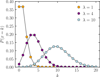
[edit | edit source]Probability mass function The horizontal axis is the index k, the number of occurrences. The function is only defined at integer values of k. The connecting lines are only guides for the eye. | |
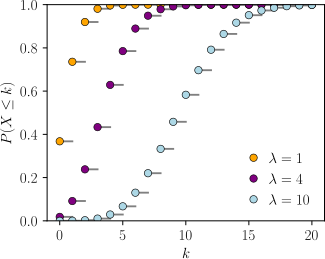
Cumulative distribution function The horizontal axis is the index k, the number of occurrences. The CDF is discontinuous at the integers of k and flat everywhere else because a variable that is Poisson distributed only takes on integer values. | |
| Notation | |
|---|---|
| Parameters | λ > 0 (real) |
| Support | k ∈ { 0, 1, 2, 3, ... } |
| PMF | |
| CDF | --or--
(for where is the Incomplete gamma function and is the floor function) |
| Mean | |
| Median | |
| Mode | |
| Variance | |
| Skewness | |
| Ex. kurtosis | |
| Entropy |
(for large )
|
| MGF | |
| CF | |
| PGF | |
Any French speaker will notice that "Poisson" means "fish", but really there's nothing fishy about this distribution. It's actually pretty straightforward. The name comes from the mathematician Siméon-Denis Poisson (1781-1840).
The Poisson Distribution is very similar to the Binomial Distribution. We are examining the number of times an event happens. The difference is subtle. Whereas the Binomial Distribution looks at how many times we register a success over a fixed total number of trials, the Poisson Distribution measures how many times a discrete event occurs, over a period of continuous space or time. There isn't a "total" value n. As with the previous sections, let's examine a couple of experiments or questions that might have an underlying Poisson nature.
- How many pennies will I encounter on my walk home?
- How many children will be delivered at the hospital today?
- How many mosquito bites did you get today after having sprayed with insecticide?
- How many angry phone calls did I get after airing a particularly distasteful political ad?
- How many products will I sell after airing a new television commercial?
- How many people, per hour, will cross a picket line into my store?
- How many alien abduction reports will be filed this year?
- How many defects will there be per 100 metres of rope sold?
What's a little different about this distribution is that the random variable X which counts the number of events can take on any non-negative integer value. In other words, I could walk home and find no pennies on the street. I could also find one penny. It's also possible (although unlikely, short of an armored-car exploding nearby) that I would find 10 or 100 or 10,000 pennies.
Instead of having a parameter p that represents a component probability like in the Bernoulli and Binomial distributions, this time we have the parameter "lambda" or λ which represents the "average or expected" number of events to happen within our experiment. The probability mass function of the Poisson is given by
- .
An example
[edit | edit source]We run a restaurant and our signature dish (which is very expensive) gets ordered on average 4 times per day. What is the probability of having this dish ordered exactly 3 times tomorrow? If we only have the ingredients to prepare 3 of these dishes, what is the probability that it will get sold out and we'll have to turn some orders away?
The probability of having the dish ordered 3 times exactly is given if we set k=3 in the above equation. Remember that we've already determined that we sell on average 4 dishes per day, so λ=4.
Here's a table of the probabilities for all values from k=0..6:
| Value for k | Probability f(k) |
| 0 | 0.0183 |
| 1 | 0.0733 |
| 2 | 0.1465 |
| 3 | 0.1954 |
| 4 | 0.1954 |
| 5 | 0.1563 |
| 6 | 0.1042 |
Now for the big question: Will we run out of food by the end of the day tomorrow? In other words, we're asking if the random variable X>3. In order to compute this we would have to add the probabilities that X=4, X=5, X=6,... all the way to infinity! But wait, there's a better way!
The probability that we run out of food P(X>3) is the same as 1 minus the probability that we don't run out of food, or 1-P(X≤3). So if we total the probability that we sell zero, one, two and three dishes and subtract that from 1, we'll have our answer. So,
- 1 - P(X≤3) = 1 - ( P(X=0) + P(X=1) + P(X=2) + P(X=3) ) = 1 - 0.4335 = 0.5665
In other words, we have a 56.65% chance of selling out of our wonderful signature dish. I guess crossing our fingers is in order!
Mean
[edit | edit source]We calculate the mean as follows:
Remember that
Variance
[edit | edit source]We derive the variance using the following formula:
We have already calculated E[X] above, so now we will calculate E[X2] and then return to this variance formula:
- ....replacing with
The first sum is E[X]=λ and the second we also calculated above to be 1.
Returning to the variance formula we find that


![{\displaystyle \lambda [1\!-\!\log(\lambda )]\!+\!e^{-\lambda }\sum _{k=0}^{\infty }{\frac {\lambda ^{k}\log(k!)}{k!}}}](https://wikimedia.org/api/rest_v1/media/math/render/svg/c5a542aefbd87a7fa233e3dad33e318fe668c637)


![{\displaystyle \operatorname {E} [X]=\sum _{i}f(x_{i})\cdot x_{i}=\sum _{x=0}^{\infty }{\frac {e^{-\lambda }\lambda ^{x}}{x!}}x}](https://wikimedia.org/api/rest_v1/media/math/render/svg/88402e8d115e24abf49290cfa3db1bb145a57a5d)
![{\displaystyle \operatorname {E} [X]={\frac {e^{-\lambda }\lambda ^{0}}{0!}}\cdot 0+\sum _{x=1}^{\infty }{\frac {e^{-\lambda }\lambda ^{x}}{x!}}x}](https://wikimedia.org/api/rest_v1/media/math/render/svg/81ef638a64528af583092231619a2dfbfef2e200)
![{\displaystyle \operatorname {E} [X]=0+e^{-\lambda }\sum _{x=1}^{\infty }{\frac {\lambda \lambda ^{x-1}}{(x-1)!}}}](https://wikimedia.org/api/rest_v1/media/math/render/svg/751d62a1284ff1725f65182e221a4fcc0f74965b)
![{\displaystyle \operatorname {E} [X]=\lambda e^{-\lambda }\sum _{x=1}^{\infty }{\frac {\lambda ^{x-1}}{(x-1)!}}}](https://wikimedia.org/api/rest_v1/media/math/render/svg/69619395b2ca4cf5c081a36f71f4e6b0ade6fd84)
![{\displaystyle \operatorname {E} [X]=\lambda e^{-\lambda }\sum _{x=0}^{\infty }{\frac {\lambda ^{x}}{x!}}}](https://wikimedia.org/api/rest_v1/media/math/render/svg/74145023b4379bed6d5237576462e1809ae4ef94)

![{\displaystyle \operatorname {E} [X]=\lambda e^{-\lambda }e^{\lambda }=\lambda }](https://wikimedia.org/api/rest_v1/media/math/render/svg/8d6908567dcb59933e108c555d132e0c0900e119)
![{\displaystyle \operatorname {Var} [X]=\operatorname {E} [X^{2}]-(\operatorname {E} [X])^{2}}](https://wikimedia.org/api/rest_v1/media/math/render/svg/d3a927c2af9ce191701ce464bf66fe7a6fe2190c)
![{\displaystyle \operatorname {E} [X^{2}]=\sum _{i}f(x_{i})\cdot x^{2}}](https://wikimedia.org/api/rest_v1/media/math/render/svg/9b457462143b3c9a9d2d1c9de47dd57fae3dbec2)
![{\displaystyle \operatorname {E} [X^{2}]=\sum _{x=0}^{\infty }{\frac {e^{-\lambda }\lambda ^{x}}{x!}}x^{2}}](https://wikimedia.org/api/rest_v1/media/math/render/svg/f093880fd23b0e728225f0aedf91b737205b6881)
![{\displaystyle \operatorname {E} [X^{2}]=0+\sum _{x=1}^{\infty }{\frac {e^{-\lambda }\lambda \lambda ^{x-1}}{(x-1)!}}x}](https://wikimedia.org/api/rest_v1/media/math/render/svg/bcdd5feeb3b4c7901689a81dce08df36c7375234)
![{\displaystyle \operatorname {E} [X^{2}]=\lambda \sum _{x=0}^{\infty }{\frac {e^{-\lambda }\lambda ^{x}}{x!}}(x+1)}](https://wikimedia.org/api/rest_v1/media/math/render/svg/7655130ce83af142e40df27e2d291c132f8251a6)


![{\displaystyle \operatorname {E} [X^{2}]=\lambda \left[\sum _{x=0}^{\infty }{\frac {e^{-\lambda }\lambda ^{x}}{x!}}x+\sum _{x=0}^{\infty }{\frac {e^{-\lambda }\lambda ^{x}}{x!}}\right]}](https://wikimedia.org/api/rest_v1/media/math/render/svg/fba5b95eea7dffc5a6c9d511b257ad1d3443827b)
![{\displaystyle \operatorname {E} [X^{2}]=\lambda \left[\lambda +1\right]=\lambda ^{2}+\lambda }](https://wikimedia.org/api/rest_v1/media/math/render/svg/1946c015894a4ec0d0122dcf9fa2ce22d3564618)
![{\displaystyle \operatorname {Var} [X]=(\lambda ^{2}+\lambda )-(\lambda )^{2}=\lambda }](https://wikimedia.org/api/rest_v1/media/math/render/svg/cc4acacd6ba940c2ba0b000304f7deae6e3e2462)