Planet Earth/4c. Carbon Dioxide in the Atmosphere
Mysterious Deaths
[edit | edit source]Her body was found when the vault was opened. Ester Penn lay inside the large locked bank vault at the Depository Trust Building on 55 Water Street in Lower Manhattan, New York. Security cameras revealed that no one had entered or left the bank vault after 9pm. Her body showed no signs of trauma, no forced entry was made into the vault, and nothing was missing. Ester Penn was a healthy 35-year old single mother of two, who was about to move into a new apartment in Brooklyn that overlooked the Manhattan skyline. Now she was dead.
On August 21, 1986, the small West Africa villages near Lake Nyos became a ghastly scene of death, when every creature, including 1,746 people, within the villages died suddenly in the night. The soundless morning brought no sounds of insects, no cries of roosters nor children playing in the streets. Everyone was dead.
Each mysterious death has been attributed to carbon dioxide toxicity. The human body can tolerate levels up to 5,000 ppm or 0.5% carbon dioxide, but levels above 3 to 4% can be fatal. A medical condition called hypercapnia occurs when the lungs are filled with elevated carbon dioxide, which causes respiratory acidosis. Normally, the body is able to expel carbon dioxide produced during metabolism through the lungs, but if there is too much carbon dioxide in the air, the blood will become enriched in carbonic acid (CO2 + H2O → H2CO3), resulting in partial pressures of carbon dioxide above 45 mmHg.
For the villagers around Lake Nyos, carbon dioxide was suddenly released from the lake where volcanic gasses had enriched the waters with the gas, while in the case of Ms. Penn, she released the carbon dioxide when she pulled a fire alarm from within the vault, which trigger a spray of carbon dioxide as a fire suppressant.[1] Divers, submarine operators, and astronauts all worry about the effects of too much carbon dioxide in the air they breathe. No more dramatic episode in carbon dioxide can match the ill-fated Apollo 13 mission to the moon.
“Houston, we have a problem.”
[edit | edit source]On April 14, 1970, at 3:07 Coordinated Universal Time 200,000 miles from Earth, three men wedged in the outbound Apollo 13 spacecraft heard an explosion.[2] A moment later astronaut Jack Swigert transmitted a message to Earth “Houston, we’ve had a problem here.” One of the oxygen tanks on board the Service Module had exploded, which also ripped a hole in a second oxygen tank, and cut power to the spacecraft. Realizing the seriousness of the situation, the crew quickly scrabbled into the Lunar Module. The spacecraft was too far from Earth to turn around. Instead the crew would have to navigate the spacecraft around the far side of the moon, and swing it back to Earth if they hoped to return alive. The Lunar Module now served as a life raft strapped to a sinking ship, the Service Module. The improvised life-raft was not designed to hold a crew of 3 people for the 4-day journey home. Oxygen was conserved by powering down the spacecraft. Water was conserved by shutting off the cooling system, and drinking became rationed to just a few ounces a day. There remained an additional worry; the buildup of carbon dioxide in the space capsule. With each out breath, the crew expelled air with about 5% carbon dioxide. This carbon dioxide would build up in the lunar module over the four-day journey, and result in death by hypercarbia; the buildup of carbon dioxide in the blood. The crew had to figure out how long the air would remain breathable in the capsule.

From Earth, television broadcasters reported the grave seriousness of the situation from Mission Control. The crew of Apollo 13 had to figure out the problem of the rising carbon dioxide in the air of the Lunar Module, if they were going to see Earth alive again.
The Keeling Curve
[edit | edit source]
In 1953, Charles “Dave” Keeling, arrived at CalTech in Pasadena, California, on a postdoctoral research grant to study the extraction of uranium from rocks. Assigned to the lab of Harrison Brown, his lab supervisor proved to be a dynamic figure. His advisor had a central role in the development of nuclear bombs used in Japan. During the war, he had invented a new way to produce plutonium, which allowed upwards of 5 kg (11 lbs) of plutonium to be added to “Fat Man” bomb that was dropped on the city of Nagasaki killing nearly 100,000 people in August 1945. After the event, Brown’s heart was crushed at the personal responsibility he felt for these deaths. He penned a book Must Destruction Be our Destiny? in 1945, and began traveling around the world giving lectures on the dangers of nuclear weapons. Harrison Brown had previously advised Claire Patterson, who was the first to radiometrically date meteorites to determine the age of the Earth at 4.5 billion years using lead isotopes while at the University of Chicago. In 1951, Harrison Brown divorced his wife and remarried, took a teaching position at Caltech, and it was here that a new chemistry postdoctoral researcher Charles Keeling arrived in 1953 to his lab. Initially, Keeling was set to the task of extracting uranium from rocks, but his interests turn to atmospheric sciences looking at the chemical composition of the air, in particular measuring the amount of carbon dioxide.
Keeling set about making an instrument in the lab to measure the amount of carbon dioxide in air using a tool called a manometer. A manometer is a cumbersome series of glass tubing which measures the pressures of isolated air samples. Air samples were captured by using a glass spherical flask, cleared of air in a vacuum and locked closed. Wrapped in canvas, so that fragile glass would not break, the empty glass spherical flask would be opened outside, and the captured gas that flowed into the glass flask would be taken back to the lab to be analyzed. The manometer was first developed to measure the amount of carbon dioxide produced in chemistry experiments involved in the combustion of hydrocarbons, allowing chemists to known how much carbon was in a material. Keeling used the same techniques to determine the amount of carbon dioxide in the atmosphere, his first measured value was 310 ppm, or 0.0310% which he found during a series of measurements made at Big Sur near Monterey, California.
Interestingly, Keeling found that concentrations of carbon dioxide increased slightly during the night. One hypothesis was that as the gas became cooler, it sank during the colder portions of the day. Carbon dioxide, which has a molar mass of 44.01 g/mol, compared to a molar mass of 32 g/mol for oxygen gas (O2) and 28 g/mol for nitrogen gas (N2), is a significantly heavier gas and will sink into lower altitudes, valleys and basins. Unless the sample was taken from places where carbon was being combusted in power plants, factories or near highways, repeated experiments showed that carbon dioxide did not vary from place to place and remained near 310 ppm.
However, this diurnal cycle intrigued him and he undertook another analysis to measure the isotopic composition of the carbon, to trace where the carbon was coming from. The ratio between Carbon-13 (13C) to Carbon-12 (12C) [this is called delta C-13 or ] is higher in molecules composed of carbon bonded to oxygen, while the ratio is lower in molecules composed of carbon bonded to hydrogen, because of the atomic difference in mass. Changes in this ratio demonstrate the source of the carbon in the air. If decreases, the source of carbon is from molecules composed of hydrocarbons, including burning or combustion of organic compounds (wood, petroleum, coal, natural gas), while if increases, the source of carbon is from molecules composed of carbonates, including burning or combustion of limestone and other rocks from volcanic emissions. Keeling found using a graph called a “Keeling Plot,” that as atmospheric carbon dioxide increased in the air, the value of decreased. This indicated that the primary source or flux of carbon dioxide in the atmosphere is primarily the interchange with organic compounds or hydrocarbons. The change in daily values, appeared to be caused by the drawdown of carbon dioxide by photosynthesizing plants during the light of the day, which was not carried out during the darkness of night, allowing carbon dioxide to increase at night.

Eagerly, Keeling wanted to take this study to the next level by looking at yearly or annual changes in atmospheric carbon dioxide. He wrote grant proposals to further his study and was awarded funds by the Weather Bureau as part of the International Geophysical Year (1957–1958). Using these funds Keeling purchased four new infrared gas analyzers. Since carbon dioxide absorbs light waves between four peaks at 1437, 1955, 2013, and 2060 nanometers in the infrared spectrum of light, light waves at these wavelengths will be absorbed by a gas that contains carbon dioxide, and the number of photons at these wavelengths can be measured to determine how much carbon dioxide is within the air. Using this more advanced tool, Keeling hoped to collect measurements from remote locations around the world. Two of the locations proposed to measure the yearly cycle was at the South Pole station in Antarctica and on top of Mauna Loa in Hawaii. Hawaii was a little more conducive to staffing personal for a full year, compared to Antarctica, and only a few measurements were made from ships that passed near the South Pole in 1957. The first measurements using the new machine from Hawaii was 313 ppm (0.0313%) taken in March of 1958. For the next year, Keeling and his staff measured the changes in carbon dioxide. From March 1958 to March 1960, Keeling measured a rise up to 315 ppm and drop down to 310 ppm indicating an oscillating cycle of rising and falling carbon dioxide due to the seasons.

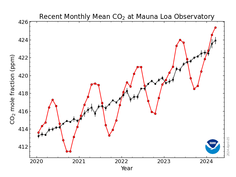
The photosynthesizing biosphere of the planet is unequally balanced across Earth, with most of the dense boreal forests positioned in the Northern Hemisphere. During the Northern Hemisphere spring and summer, carbon dioxide is pulled from the atmosphere as these dense forest plants grow and become green during the spring and summer days, while in the fall and winter in the Northern Hemisphere carbon dioxide returns back to the atmosphere as autumn leaves fall from trees in these deciduous forests, and plants prepare to go dormant for the cold winter. As an annual cycle, the amount of carbon dioxide in the atmosphere is a rhythmic pulse, increasing and decreasing, with the highest levels in February, and lowest levels in late August.

After funding from the International Geophysical Year had expired, funds were provided by the Scripps Institution of Oceanography program, but in 1964 congressional budget cuts nearly closed the research down. Dave Keeling worked relentlessly to secure funding to maintain the collection of data receiving grants and funding from various government agencies. His dogged determination likely stemmed from the discovery that carbon dioxide each year was increasing at a faster and faster rate. In 1970, the carbon dioxide in Hawaii was at 328 ppm (0.0328%), in 1980 at 341 ppm (0.0341%), in 1990 at 357 ppm (0.0357%), and in 2000 at 371 ppm (0.0371%). In 2005, Dave Keeling passed away, but the alarming trend of the increasing amount of carbon dioxide had captured the attention of the public. In 2006, Al Gore produced the documentary “An Inconvenient Truth” about the rise of carbon dioxide in the atmosphere, stemming from Keeling’s research and a prior scientific report made in 1996, when he was Vice President. The ever-increasing plot of carbon dioxide in the atmosphere, became known as the Keeling curve. Like the air in the capsule of Apollo 13, the amount of carbon dioxide was increasing dramatically. Today in 2020, carbon dioxide has risen above 415 ppm (0.0415%) in Hawaii. By extending the record of carbon dioxide back in time using air bubbles trapped in ice cores, carbon dioxide has doubled in the atmosphere from 200 ppm to over 400 ppm, much of the increase in the last hundred years.

Isotopic measurements document where much of this increase in carbon dioxide is coming from. values are more negative today than they have ever been, indicating emission of carbon dioxide dominantly from hydrocarbons (organic molecules of carbon), such as wood, coal, petroleum and natural gas. The ever-increasing human population, and exponential use of hydrocarbon fuels, coupled with deforestation and increased wild fires is the source of this increased carbon dioxide. This increase is far greater than the carbon dioxide that is annually drawn down by spring regrowth of forests in the Northern Hemisphere. Just like oxygen dramatically changed the atmosphere of the Proterozoic, the exponential release of carbon dioxide is dramatically changing the atmosphere of Earth today.
In the last twenty years, scientists have begun measuring carbon dioxide in the atmosphere from a wider variety of locations. In Utah, more than a dozen stations today monitor carbon dioxide in the atmosphere. In Salt Lake City, carbon dioxide in 2020 typically spikes to values near 700 ppm (0.07%) during January and February, as a result of carbon dioxide gas sinking into the valleys along the Wasatch Front and the large urban population using hydrocarbon fuels, while values in Fruitland, in rural Eastern Utah, have high values near 500 ppm (0.05%). This means that carbon dioxide measured from Hawaii, as part of the Keeling Curve, is minimal compared to Utah, given that the island’s isolated location in the Pacific Ocean. Values found in urban cities can be nearly twice the amount of carbon dioxide compared to those currently observed on the Hawaii Island monitoring station. This makes these urban centers especially a health risk with people suffering from respiratory distress syndrome associated with diseases such as the coronavirus that killed over 200,000 Americans in 2020.
In 2009, NASA’s planned launch of the Orbiting Carbon Observatory satellite, met with failure on the launch pad and was lost. In 2014, the Orbiting Carbon Observatory-2 satellite was more successful, and provided some of the best measurements of carbon dioxide from space using infrared light absorption across the entire Earth. Dramatically, carbon dioxide is most abundant in the atmosphere above the Northern Hemisphere compared to the Southern Hemisphere, with the highest concentration of carbon dioxide during the winter months in eastern North America, Europe and eastern Asia. Carbon dioxide is mostly concentrated below 15 to 10 kilometers in the atmosphere, and rises dramatically from major urban centers and large forest fires. The Orbiting Carbon Observatory-3 was successfully launched into space in 2019, and is installed on the International Space Station. This instrument measures carbon dioxide on a finer scale than the OCO‑2, while also looking at reflected light from vegetation to monitor global desertification.
Predicting Carbon dioxide in the atmosphere of the future
[edit | edit source]
Albert Bartlett was a wise old professor at the University of Colorado’s physics department who spent his scientific career on one key aspect: Teaching students how to understand the exponential function. What is an exponential function and how does it relate to predictions of carbon dioxide in the atmosphere of Earth’s future? An exponential function is best described in a famous Persian story, first told by Ibn Khallikan in the 13th century.
A variation of the story goes something like this: A wealthy merchant had a lovely daughter, who the king desired to marry. The merchant, knowing of how much the king was in love with his daughter offered him a deal. In 64 days, he could marry his daughter if on a chessboard, each day the king was to pay him one penny for each square. However, each day he would have to double the number of pennies from the prior square, until he filled all 64 squares on the chessboard. The king had millions of dollars in his vault, filling a chessboard with pennies was easy. He agreed. On the first day, the king lay down one penny on the first square. He laughed at how small the number was on the second day as the king lay down 2 pennies, and on the third day only 4 pennies. He laughed and laughed, he had only spent a total of 7 cents, and it was already going on day four, when he lay down 8 pennies, but things started to change on the second row of the chessboard, by the 16th day he had to lay out 32,768 pennies, or $327.68. By the third row, the values increased more dramatically to fill the next row he had to cough up $42,949,672.96, or more than 42 million dollars and to fill the fourth row, he had to come up with $10,995,116,277.76, or 10 billion dollars. In fact, if the king was to fill all 64 squares, the last square would total $184,467,440,737,100,000.00, or over 184 trillion dollars! He ran out of money, and could not afford to marry the merchant’s daughter. Exponential functions can work in the opposite direction too, such as halving the number, as observed with radiometric decay used in dating.
The critical question that involves carbon dioxide in the Earth’s atmosphere, is whether it is growing exponentially or linearly over time? One way to test this is to write a mathematical function that best explains the growth of carbon dioxide in the atmosphere, which can be used to project its future growth. With the complete data set from the Keeling Curve, from 1958 to the present, we can use this data to make some predictions of carbon dioxide in the future. The annual mean rate of growth of CO2 for each year is the difference in concentration between the end of December and the start of January of each year. Between 1958-1959 the rate of growth was 0.94 ppm, but between 2015-2016 the rate of growth jumped to 3.00 ppm. In the last twenty years, the rate of growth has not been less than 1.00 ppm. Indicating an upward trend of growth, more like that seen in an exponential function.
The best fit mathematical equation using the mean or average carbon dioxide from Hawaii each year works out to be a more complex polynomial exponential function.

This approximate model explains the data recorded since 1958, which can be applied to the future. As a model, it is only good as a prediction and serves only as a hypothesis that can be refuted with continued data collection each year into the future. Using this mathematical model, we can insert any year, and see what the predicted value in carbon dioxide would be. For the year 2050, the predicted value of carbon dioxide would be 502.55 ppm with an annual growth rate of 3.28 ppm per year. Like the king in the story, you may laugh at this value. Compared to 2020 values around 410 ppm, it is well below the dangerous values which would make the air unbreathable around 1 to 4% or 10,000 ppm to 40,000 ppm. In fact, the air would be breathable as 502.55 ppm is only 0.05%. The growth rate, would be accelerating each year. In 2100, eighty years from this authorship of this text, the predicted value would be 696.60 ppm, with a 4.50 ppm annual growth rate.
This likely would be worse in major cities, like Salt Lake City, which would experience cold winter days of bad air-days with carbon dioxide about 1,000 ppm. While not fatal, such high values might cause health problems to citizens with poor respiration, such as new born infants, people suffering from viral respiratory diseases like the corona virus and influenza, elderly people with asthma, and diabetes. The next jump to the year 2150, predicts a level of 954.15 ppm, with a growth rate of 5.77 ppm. At this point, most of the Northern Hemisphere would contain unhealthy air. Sporting events and outdoor recreation would be unadvisable, although people could still breath outdoor air, air filtration systems would likely be developed to keep carbon dioxide levels lower indoors. In the 23rd century, things begin to get worse. Carbon dioxide would reach 1,275.20 ppm with an annual growth of 7.04 ppm each year. At this point, topographic basins and cold regions near sea level would cause respiratory issues, especially on cold January and February nights.
By the year 2300, carbon dioxide would be at levels around 2,107.80 ppm or 0.2%, with a growth rate of 9.58 ppm. At this point, people could only spend limited time outside, before coming home to filtered air with lower carbon dioxide. Sporting events would move inside, as exertion would cause respiratory failure. In the year 2400, carbon dioxide would be at 3,194.40 ppm or 0.3% with an annual growth of 12.12 ppm, and by the year 2500, carbon dioxide would be at 4,535.00 ppm, with an annual growth of 14.66 ppm per year. At this point, beyond the healthy recommended dose for 8-hours, the outside air would become nearly unbreathable for extended periods of time.
By the year 2797, the level of carbon dioxide would reach 1% in Hawaii, or 10,000 ppm leading to an atmosphere unbreathable, across much of the Northern Hemisphere. Millions and billions of people would die across the planet, unable to breathe the air on days when carbon dioxide would rise above the threshold. If this model holds, and the predication is correct, Earth will be rid of humans and most animal life in the next 777 years. This is a small skip of time, as the story of the chessboard was first written down by the Persian scholar Ibn Khallikan, about the same length of time in the past. If a scholar living in the 13th century wrote an allegory that is still valid today, what words of knowledge are you likely to pass on to future generations in the 28th century? Is this mathematical model a certainty toward the ultimate track to human extinction?
One of the great scholars of exponential growth, was Donella Meadows, who wrote in her 1996 essay “Envisioning a Sustainable World":
“We talk easily and endlessly about our frustrations, doubts, and complaints, but we speak only rarely, and sometimes with embarrassment, about our dreams and values.”
It is vital to realize that a sustainable world, where carbon dioxide does not rise above these thresholds, that you, and the global community advert this rise in carbon dioxide, while Earth is on the first few squares of this global chessboard. If you would like to play with various scenarios of adverting such a future, check out the Climate Interactive website, https://www.climateinteractive.org, and some of the computer models based on differing policy reductions in carbon dioxide released into the atmosphere. Donella Meadows further wrote, that
“The best goal most of us who work toward sustainability offer is the avoidance of catastrophe. We promise survival and not much more. That is a failure of vision.”
It sounds very optimistic, and having been written nearly twenty-five years ago, when carbon dioxide was only 362 ppm, seems a mismatch to more urgent fears today as carbon dioxide has reached 410 ppm in the atmosphere, and so much like the Apollo 13 mission, you, and everyone you love, are trapped in a space capsule breathing in a rapidly degrading atmosphere.
Was it ever this high? Carbon dioxide in ancient atmospheres
[edit | edit source]One of the criticisms of such mathematical models is that there is a finite amount of carbon on Earth, and that resources of hydrocarbons (wood, coal, petroleum, and natural gas) will be depleted well before these high values will be reached. Geological and planetary evidence from Mars and Venus, as well as the evidence regarding the atmosphere of the Archean Eon, indicate that high percentages of carbon dioxide upwards of 95% is possible if the majority of Earth’s carbon is released back into the atmosphere. Such a carbon dioxide dominant atmosphere is unlikely, given that such release would require all sequestered calcium carbonate to be transformed to carbon dioxide. However, there have been periods in Earth’s past that carbon dioxide levels were higher than they are today.

Measurement of air samples only extends back some 800,000 years, since ice core data, and the bubbles of air they trap, are only as old as the oldest and deepest buried ice in Greenland and Antarctica. Values from ice cores demonstrate that carbon dioxide for the last 800,000 years varied only between 175 to 300 ppm, and never appeared above 400 ppm, like today’s values. If we want to look at events in the past where carbon dioxide was higher, we have to look back in time, millions of years. However, directly measuring air samples is not possible the farther back in time you go, so scientists have had to develop a number of proxies to determine carbon dioxide levels in the distant past.
The Stomata of Fossil Leaves
[edit | edit source]
Photosynthesis in plants requires gas exchange where carbon dioxide is taken in and oxygen is released. This gas exchange in plants happens through tiny openings on the bottom-side of leaves called stomata. The number of stomata in leaves is balanced, because the more carbon dioxide is in the air the fewer the number of stomata is needed, while less carbon dioxide in the air will result in more stomata. Plants need to minimize the number of stomata used for gas exchange, because an excess of stomata will lead to water loss and the plant will dry out.


Looking at fossil leaves under microscopes and counting the number of stomata per area, as well as greenhouse experiments calibrating plants grown with controlled values of carbon dioxide have allowed scientists to be able to extend the record of carbon dioxide in the atmosphere back in time. There are a few limitations to this method. First is that only plants living both today and in the ancient past can be used. Most often these experiments use Ginkgo and Metasequoia leaves, which are living fossil plants with long fossil records extending back over 200 million years. Leaves of these plants have to be found as fossils, with good preservation for specific periods of time. The proxy works best with carbon dioxide concentrations between 200 ppm to about 600 ppm. High values above 600 ppm, the number of stomata has decreased to a minimum, and there is not much gained for the plant to have fewer openings with such high concentrations of carbon dioxide. Published values above 600 ppm all likely have similar or nearly the same density of stomata. A plant grown in 800 ppm carbon dioxide would have similar density of stomata as a plant grown in 1,500 ppm. This makes it difficult to calculate carbon dioxide in ancient atmospheres, when values are high, above 600 ppm.
Studies of fossil leaves, coupled with other proxies for atmospheric carbon dioxide in the rock record demonstrate that carbon dioxide has remained below 500 ppm over the last 24 million years, although near 16.3 million years ago, during the Middle Miocene Climate Optimum values are thought to have been between 500 and 560 ppm, and fossil evidence of warmer climates has been observed during this period of time. During this period ice sheets where absent in Greenland, and much of western North America and Europe was covered in arid environments, and savannah-like forests seen today in southern Africa.

Extending further back, during the Eocene Epoch between 55.5 and 34 million years ago, carbon dioxide values are thought to have been much higher than today, above 600 ppm. The Eocene Epoch was a particular warm period during Earth’s past. Crocodile fossils are abundant in Utah, as well as fossil palms. The environment of Utah was similar to Louisiana is today, wet and humid, with no snow observed in the winter as evidence by the lack of glacial deposits. The warmer climate allowed crocodiles, early primates and semitropical forests to flourish in eastern Utah, and across much of North America, in many places today that are cold dry deserts. The buildup of carbon dioxide gradually peaked at about 50 million years ago, during the Early Eocene Climate Optimum. During this time large conifer forests of Metasequoia grew across the high northern Arctic, which was inhabited by tapirs. A much more abrupt event happened 55.5 million years ago, called the Paleocene-Eocene Thermal Maximum, in which carbon dioxide is thought to have doubled over a short duration of about 70 thousand years. The Paleocene-Eocene Thermal Maximum, or PETM is thought to have raised carbon dioxide values in the atmosphere above 750 ppm, and likely upward to 1,000 to 5,000 ppm. Values returned to lower amounts afterward to about 600 ppm. The climate drastically changed, resulting in a major turnover of mammals living at the time. The oceans became acidic, with elevated amounts of carbonic acid, and there is evidence that average global temperatures rose between 6 to 8 degrees Celsius. Methane released from the sea floor of the Arctic Ocean due to volcanism below the northernmost region of the North Atlantic Ocean likely caused the increase in carbon dioxide in the atmosphere. This was further enhanced by a positive feedback, as the warmer and drier climate resulted in massive forest fires that erupted across the Northern Hemisphere, as evidenced by the extinction of many tree dwelling mammals. Modern primates arose from the burned embers of this global event and came to dominate the eventual return of forests of the later Eocene Epoch. Eocene primates, as humanity’s ancestors were the survivors of this catastrophic global warming event.

In the age of dinosaurs, carbon dioxide varied higher than in the age of mammals. In the late Cretaceous, Tyrannosaurus rex breathed in air that likely was composed of 500-600 ppm carbon dioxide, based on stomata in fossil leaves found alongside the dinosaur. However, the asteroid impact at the end of the Cretaceous resulted in spikes of carbon dioxide reaching approximately 1,600 ppm. The age of dinosaurs was a long period of 186 million years in which glaciers are completely absent from the geological record, and there is no evidence of polar ice sheets. Around 125 million years ago, carbon dioxide levels skirted above 1,000 to 1,500 ppm, while in the Jurassic Period levels where likely near 1,000 ppm, and at least above the 600 ppm threshold. The Triassic Period, and in particular near the Triassic-Jurassic boundary, 200 million years ago, values of carbon dioxide were very high, with 1,000 ppm up to 2,500 ppm, and likely higher due to volcanism associated with the opening of the Atlantic Ocean. Utah, and much of Western North America was part of a gigantic vast desert. A desert that was extremely hot and dry, despite being close to the ocean. Like Saudi Arabia today, Utah was covered in massive sand dunes (a sand sea or erg) during the Triassic and Jurassic Periods, leaving behind rock layers made from these ancient sands that form the geological arches in Arches National Park near Moab, Utah, and deep canyons of Zion National Park near Springdale, Utah. The record becomes more challenging to uncover going even farther back in time, no longer are modern plants found, and the record of carbon dioxide must be reconstructed using other tools. However, evidence suggests that carbon dioxide remained below the 5,000 ppm threshold, and when levels rose above 2,000 ppm it often led to major extinctions, such as during the PETM event and Triassic-Jurassic Boundary, and levels above 1,500 ppm, with the extinction of the dinosaurs 66 million years ago.
Carbon Isotopes
[edit | edit source]
As discussed previously, when carbon dioxide increases in the atmosphere, the isotopic ratio of Carbon-13 to Carbon-12 decreases, because much of this carbon comes from hydrocarbon molecules, carbon bonded to hydrogen. Geologists can measure the ratio of carbon isotopes in the rocks. However, to equate the isotopic carbon ratio in rocks to the amount of carbon dioxide in the atmosphere is complex. For example, if rocks that contain calcium carbonate are examined, the ratio will be high, because the carbon is bonded to oxygen, while if rocks that contain organic carbon are examined, such as coal, the ratio will be low, because the carbon is bonded to hydrogen. You can only compare values from similar types of rocks. However, different trees and different types of plants that form coal can have different carbon isotopic ratios, and it has even been shown that rocks deposited in different latitudes can have different carbon isotopes, making working out the relationship between the isotopic ratio, and what the atmosphere concentration of carbon dioxide was in the ancient past difficult. However, there is an overall relationship that lower or more negative carbon isotope ratios (more Carbon-12), indicate a higher likelihood of high levels of carbon dioxide in the atmosphere. Using this proxy, the record of carbon dioxide in the atmosphere can be extended back in time, to a period when carbon dioxide may have reached the dangerous high level of 1% (10,000 ppm) and above, making the air toxic to breathe.
The Great Dying
[edit | edit source]There is a reason that the Permian-Triassic Boundary, an event that occurred 252 million years ago, is called the Great Dying. Preserved in the rock record is catastrophic death of between 83 to 97% of life on the planet. The event is marked with an abrupt negative excursion of carbon isotopes indicating massive amounts of carbon dioxide in the atmosphere. The oceans became acidic and anoxic (lacking oxygen), and global temperatures in oceans were the highest they have been 500 million years. A massive volcanic eruption, called the Siberian Traps ignited gigantic deposits of coal, trapped petroleum and natural gas. The atmosphere became thick with sulfuric acid, mercury, and lead. Evidence of this event is scattered globally in the rock record, where a thin layer of mercury-enriched rock can be found marking the event in the sediments.
The Great Dying is geologic evidence that lethal levels of carbon dioxide in the atmosphere are possible and a real danger. Values above 1% of carbon dioxide resulted in a nearly dead world, where animal life was particularly hard hit. The recovery took millions of years, likely preventing any ice ages or ice sheets in the Arctic and Antarctic for the next 218 million years and the reason for the high values near 1,000 ppm in the Triassic and Jurassic Periods as the Earth staggered to recover from this event.
Prior to the Great Dying event, carbon dioxide values were likely below 500 ppm, in fact during the early Permian Period, and earlier Pennsylvanian and Mississippian Periods about 300 million years ago, carbon dioxide were likely much lower due to the drawdown of carbon dioxide in the atmosphere by the large carboniferous forests, which today are the source of much of the coal burned today in eastern North America, Europe and Russia. Evidence of glacial deposits during this period are known, and the world was much cooler, similar to our more recent history.
The geological evidence gathered across time demonstrates that carbon dioxide in the atmosphere can easily rise above dangerous levels, making breathing the air impossible for animals. This is especially true in a post-2020 world, where viral respiratory diseases like COVID-2019, have increased fatality rates in air high in carbon dioxide with increased risk of hypercapnia. Like the spinning space capsule of Apollo 13 hurdling through space, with alarms blinking, the air on spaceship Earth is also becoming too enriched in carbon dioxide. The crew of Apollo 13 had to solve the problem of the rising carbon dioxide, just like how you have to solve the problem of rising carbon dioxide on Earth today.
Carbon dioxide scrubbers
[edit | edit source]
To solve the carbon dioxide problem, carbon dioxide must be removed from the air. This requires passing air through a scrubber. A scrubber is a chemical reaction that reacts with carbon dioxide and releases oxygen. In space capsules, the scrubbers are composed of lithium hydroxide canisters, and the problem facing Apollo 13 was that the Lunar Module did not have enough lithium hydroxide canisters to remove the rising carbon dioxide. Using plastic bags, cardboard and tape, mission control developed a quick solution to the problem by allowing the trapped crew to use lithium hydroxide canisters from the Service Module inside the Lunar Module. The problem was solved with only the tools available on hand, and these lithium hydroxide canisters scrubbed the rising carbon dioxide in the space craft just enough to get the crew home to Earth safely.
What are the carbon dioxide scrubbers of Earth’s air? To solve this global problem, some engineers propose inventing mechanic or chemical scrubbers, like gigantic lithium hydroxide canisters, others proposes genetically modified organisms, but the truth is that Earth’s carbon dioxide scrubbers are all around us: photosynthesizing lifeforms. The health of your planet and your own existence is locked with the health of the Earth’s forests, vegetation, gardens, soils, and even the phytoplankton of the oceans. All photosynthesizing lifeforms convert carbon dioxide to oxygen. They are and have always been Earth’s great scrubbers of carbon dioxide from the atmosphere.
| Previous | Current | Next |
|---|---|---|