MATLAB Programming/Vector and Matrices/Operations on Matrices

Basic Matrix Operation

Addition and subtraction

We can add and subtract the matrices if both of them are of same number of rows and columns.

Examples as follows:

  >> a = [7,9,4;6,2,5]
  a =
     7     9     4
     6     2     5

  >> b=[2,0,1;4,7,3]
  b =
     2     0     1
     4     7     3

  >> % Addition of a and b matrices
  a+b
  ans =
     9     9     5
    10     9     8

  >> % Subtraction of a and b matrices
  a-b
  ans =
     5     9     3
     2    -5     2

Matrix multiplication

For matrix multiplications, there are 2 ways to do multiplications.

(i) Matrix multiplications (using symbol * or mtimes)

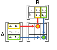
Requirements is that the number of columns in the first matrix must be same as the number of rows in the second matrix.

As examples shown on the right , matrix A have 3 X 2 and matrix B have 2 X3

Therefore , 2 X 3 <-> 3 X 2 , hence, it fulfils the requirements above.

Also, take note that the resulting matrix sizes is based on number of rows of first matrix with number of columns in second matrix.

>> A=[4,2,4;8,3,1]

A =
     4     2     4
     8     3     1

>> B=[3,5;2,8;7,9]

B =
     3     5
     2     8
     7     9

>> mtimes(A,B)

ans =
    44    72
    37    73

>> A*B

ans =

    44    72
    37    73

Following examples shows what if the incorrect matrix dimension matches.

As shown, the matrix C have 5X4 and matrix D have 3X2

5X 4 <-> 3X2, therefore it cannot fulfill the conditions and unable to solve it.

>> %Demonstrations what if matrices dimensions are incorrect 
>> C=randi(10,5,4)

C =

     2    10    10     3
     2    10     4     5
     3     5     2     1
     5     5     8     2
     1     4     4    10

>> D=randi(10,3,2)

D =

    10     3
     6     4
     1     9

>> mtimes(C,D)
Error using  * 
Incorrect dimensions for matrix multiplication. Check that the number of columns in the first
matrix matches the number of rows in the second matrix. To perform elementwise
multiplication, use '.*'.

(ii) Dot product (Note: Only can be used if both matrices are same sizes) Taking examples above, it doesn't solve the equations as both matrix A and B above are not same size

>> A.*B % want to show dot product unable to solve this multiplication issues
Matrix dimensions must agree.

Creating Random Integer Matrix

To generate random integer matrix, can type the following randi(IMAX,M,N)
Note: IMAX is the maximum integer (starting from 1) and M*N matrix

Examples as followed:

>> randi(50,3,4)

ans =
     9    14    42    48
    36     3    35     2
     2     5    16    22

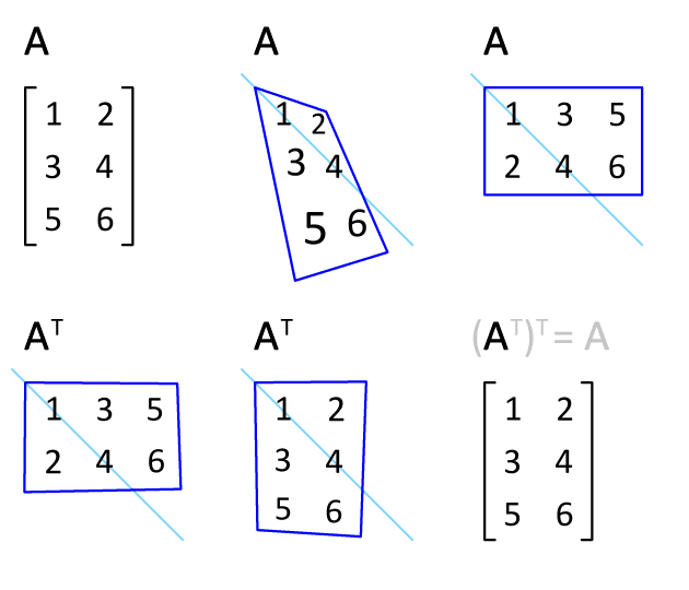
Transpose

Using the matrices above, we can transpose the matrices. Transpose matrices usually just switch the row to column and columns into rows. The picture shown just demonstrate the transpose operation. One of the application of transpose the matrix is to cryptography.

There are two ways to go about it. One is add ' to the end of the matrix that are going to be transpose or function transpose.

Back to the magic square example above, we are going to transpose it. We can see , it is transpose along the diagonal line looks like this : \

  >> % transpose matrix c to d
  >> d = c'
  d =
    17    23     4    10    11
    24     5     6    12    18
     1     7    13    19    25
     8    14    20    21     2
    15    16    22     3     9

Determinant

The determinant of matrix is a special number that is defined only for square matrices.
A determinant is used to find the solution of a system of linear equations and determine the inverse of a matrix.

Determinant of 2X2 matrix : $\mathbf {A} ={\begin{bmatrix}a&b\\c&d\\\end{bmatrix}}*|A|=ad-bc$

Determinant of 3X3 matrix : $\mathbf {A} ={\begin{bmatrix}a&b&c\\d&e&f\\g&h&i\end{bmatrix}}*|A|=a(ei-fh)-b(di-fg)+c(dh-eg)$

>> A=[6,1,1;4,-2,5;2,8,7]

A =
     6     1     1
     4    -2     5
     2     8     7

>> det(A)
ans =
 -306.0000

Inverse

Inverse of matrix is reciprocal matrix where the formula is denoted by ${A}^{-1}={\frac {1}{|A|}}adjA$
, where the adj is representing adjoint of matrix.

Note: Not all matrix have inverse, if their determinant is equal to zero.

>>%matrix inversion using manual method

>> M=[2,-1,3;-5,3,1;-3,2,3]

M =

     2    -1     3
    -5     3     1
    -3     2     3

>> %First we find the matrix determinant
>> DM = det(M)

DM =
   -1.0000

>>%Since determinant IS NOT equal to 0, we can find the matrix inverses

>> AM = adjoint(M)
AM =
    7.0000    9.0000  -10.0000
   12.0000   15.0000  -17.0000
   -1.0000   -1.0000    1.0000

>> (1/DM)*AM

ans =
   -7.0000   -9.0000   10.0000
  -12.0000  -15.0000   17.0000
    1.0000    1.0000   -1.0000

%shortcut using function inv which should be same as manual calculation above
>> inv(M)

ans =
   -7.0000   -9.0000   10.0000
  -12.0000  -15.0000   17.0000
    1.0000    1.0000   -1.0000

Real life applications

There are many applications of matrix such as:

Crytography :

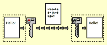
Matrix it is used to encrypt message codes. Matrices are used by programmers to code or encrypt letters. A message is made up of a series of binary numbers that are solved using coding theory for communication. As a result, the concept of matrices is used to solve such equations.

To perform this matrix operation, the message is first broken up into blocks of fixed size, and each block is represented as a vector of numbers. The public key includes a matrix, called the encryption matrix or the public matrix, that is used to transform each vector of numbers. The resulting transformed vectors are then raised to the exponent modulo the modulus to get the ciphertext.

% Define the message to encrypt
message = 'I LOVE MATLAB';

% Convert the message to a vector of numbers
message_vec = double(message);

% Define the public key parameters (modulus and exponent)
% Next, we define the public key parameters, which in this case are a modulus of 104729 and an exponent of 65537.
modulus = 104729;
exponent = 65537;

% Define the encryption matrix
% We also define an encryption matrix of size 2x2.
encryption_matrix = [3 5; 7 11];

% Break the message vector into blocks of length 2
block_size = 2;
num_blocks = ceil(length(message_vec) / block_size);
message_blocks = zeros(num_blocks, block_size);
message_blocks(1:length(message_vec)) = reshape(message_vec, [], block_size);

% Apply the encryption matrix to each message block
encrypted_blocks = mod(message_blocks * encryption_matrix, modulus);

% Raise each encrypted block to the exponent
exponentiated_blocks = mod(encrypted_blocks .^ exponent, modulus);

% Convert the encrypted blocks to a single vector of numbers
encrypted_vec = reshape(exponentiated_blocks, [], 1);

% Print out the encrypted message
fprintf('Encrypted message: %s\n', char(encrypted_vec'));

To decrypt the message, the private key is used, which consists of two parts: the modulus and the inverse of the exponent modulo a certain value. The inverse of the exponent is used to raise the ciphertext to a power that will reverse the matrix transformation and recover the original message blocks.

% Define the encrypted message
encrypted_message = [16124 4546 84313 99848 16124 4546 84313 40458 16124 4546 84313 40458 32274 40458];

% Define the private key parameters (modulus and inverse exponent)
modulus = 104729;
inverse_exponent = 47027;

% Define the decryption matrix
decryption_matrix = [17 23; 21 29];

% Break the encrypted message vector into blocks of length 2
block_size = 2;
num_blocks = length(encrypted_message) / block_size;
encrypted_blocks = reshape(encrypted_message, block_size, num_blocks)';

% Raise each encrypted block to the inverse of the exponent
decrypted_blocks = mod(encrypted_blocks .^ inverse_exponent, modulus);

% Apply the decryption matrix to each decrypted block
decrypted_blocks = mod(decrypted_blocks * decryption_matrix, modulus);

% Convert the decrypted blocks to a single vector of numbers
decrypted_vec = reshape(decrypted_blocks, [], 1);

% Convert the decrypted vector to a string and print it out
fprintf('Decrypted message: %s\n', char(decrypted_vec'));

Image Processing :

One of the matrix operations applicable in real life is image processing. We will look into one of the simpler examples such as image blurring.

For example, we want to apply blurring to an supposedly B&W image with an example of matrix shown here where each values in pixel represent a grayscale values from 1 to 255.

We will use matrix convolution to takes the average of the pixel values in a 3x3 neighborhood around each pixel in the image.

To apply this filter, we will slide the matrix over each pixel in the image and perform a matrix multiplication. For example, to blur the pixel at center in the image, you would take the 3x3 neighborhood around it, multiply each pixel value by the corresponding value in the blur filter matrix, and then add up the results. The final value is the new pixel value for the blurred image.

We repeat this process for every pixel in the image, and the result is a new image that looks blurrier.

% Define the input matrix
input_matrix = [1 2 3; 8 9 4; 7 6 5];

% Define the blur filter matrix
blur_filter = 1/9 * [1 1 1; 1 1 1; 1 1 1];

% Apply the filter using convolution
blurred_matrix = conv2(input_matrix, blur_filter, 'same');

% Display the original and blurred matrices side by side
disp('Original Matrix:');
disp(input_matrix);
disp('Blurred Matrix:');
disp(blurred_matrix);

Circuit analysis:

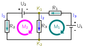
In electrical engineering, the Kirchoff's Voltage Law (KVL) states that the sum of all voltages around a closed loop in a circuit must be equal to zero. This law can be used to write a set of linear equations for a circuit with m loops. These equations can be arranged in a matrix, known as the loop-branch incidence matrix.

Based on this examples shown:

Loop M1 : V1 - R1*I1 - R3*I2 = 0

Loop M2 : V2 - R2*I2 - R3*I1 = 0

[ R1 -R3 0 ] [ I1 ] = [ V1 ]

[-R3 R2+R3 -R2 ] [ I2 ] = [ -V2 ]

[ 0 -R2 1 ] [ V2 ] = [ 0 ]

Using symbolic math tool box, we can solve the equations

% Define the symbolic variables
syms R1 R2 R3 V1 V2 I1 I2

% Define the Kirchhoff Voltage Law equations for each loop
eq1 = V1 - R1*I1 - R3*(I1-I2) == 0;
eq2 = V2 - R2*I2 - R3*(I2-I1) == 0;

% Define the Kirchhoff Current Law equation at node K1 and K2
eq3 = I1 - I2 == 0;

% Solve the system of equations for the currents and voltages
sol = solve(eq1, eq2, eq3, I1, I2, V2);

% Display the results
I1 = double(sol.I1);
I2 = double(sol.I2);
V2 = double(sol.V2);
fprintf('I1 = %.2f A\n', I1);
fprintf('I2 = %.2f A\n', I2);
fprintf('V2 = %.2f V\n', V2);

References

^[1] ^[2] ^[3] ^[4]

[1] ttps://web.archive.org/web/20220712153202/https://collegedunia.com/exams/applications-of-determinants-and-matrices-and-solved-examples-mathematics-articleid-2195

[2] ttps://web.archive.org/web/20220719154910/https://www.embibe.com/exams/inverse-matrix/

[3] ttps://web.archive.org/web/20220814062118/https://www.theclickreader.com/dot-products-and-matrix-multiplication/

[4] ttps://web.archive.org/web/20220814062138/https://www.theclickreader.com/matrix-transpose-determinants-and-inverse/

[1]

[2]

[3]

[4]