Objectives
- understand interpolation
- derive Newton’s divided difference method of interpolation
- derive Lagrangian method of interpolation
- apply the interpolation methods to solve problems
- find derivatives and integrals of discrete functions using interpolation
Resources
Interpolation is the process of deriving a simple function from a set of discrete data points so that the function passes through all the given data points (i.e. reproduces the data points exactly) and can be used to estimate data points in-between the given ones. It is necessary because in science and engineering we often need to deal with discrete experimental data. Interpolation is also used to simplify complicated functions by sampling data points and interpolating them using a simpler function. Polynomials are commonly used for interpolation because they are easier to evaluate, differentiate, and integrate - known as polynomial interpolation.
It can be proven that given n+1 data points it is always possible to find a polynomial of order/degree n to pass through/reproduce the n+1 points.
Given n+1 data points the direct method assumes the following polynomial:

With n+1 values for  and the n+1 corresponding values for
  we can solve for
  by solving the n+1 simultaneous linear equations, which is known as the direct method.
For example, given two data points  and
and  we can use a linear function
  to pass through the two data points:


Once we solve for  and
and  (the coefficients of
  ) we can use the function as the basis for interpolation - estimating the missing data points in-between.
In Newton's method the interpolating function is written in Newton polynomial(a.k.a Newton form). For example, given one data point  we can only derive a polynomial of order zero:
  . Because
  the newton polynomial of order zero is
  .
.
Given two data points we can write Newton's polynomial in the form of  . Plugging in the two data points gives us


Obviously this function passes through both data points (i.e. accurately reproduces the two data points). The first derivative of the function at  is
is  , which matches the result from the forward divided difference method.
Given three data points we can write Newton's polynomial in the form of

Plugging in the three data points gives us
- As
 we get
- As
 we get
- As

- we get

This third degree polynomial function passes all three data points (the second derivative and the third derivative at  and
and  match that from the divided difference method).
From the two examples we can see the coefficients of a Newton polynomial follow a pattern known as divided difference. For example is called divided difference of order 1 (denoted as
 ![{\displaystyle f[x_{0},x_{1}]}](https://wikimedia.org/api/rest_v1/media/math/render/svg/a31f8458da9ea4ec290a96134207b45c5d7a4f7c) ) because it depends on
) because it depends on  and
and  . The divided difference notation can be used to write the general order (form) Newton polynomial:
![{\displaystyle f(x)=f[x_{0}]+f[x_{0},x_{1}](x-x_{0})+f[x_{0},x_{1},x_{2}](x-x_{0})(x-x_{1})+...}](https://wikimedia.org/api/rest_v1/media/math/render/svg/847c840f35a86400cc5ad569d0be1c07888a60af)
(x-x_{1})(x-x_{2})...(x-x_{n-1})}](https://wikimedia.org/api/rest_v1/media/math/render/svg/58a15892e49e48dcc2f7ed29262bcfb7e0d60634)
Where
![{\displaystyle a_{0}=f[x_{0}]=y_{0}}](https://wikimedia.org/api/rest_v1/media/math/render/svg/b2c02509aa73c0099d52cc8960bd92a2bc3ab880) because
because ![{\displaystyle f[x_{i}]=y_{i}}](https://wikimedia.org/api/rest_v1/media/math/render/svg/155fee5ebbf6543462143a8a14da42bcbb14a0a3) by definition
by definition![{\displaystyle a_{1}=f[x_{0},x_{1}]={\frac {f[x_{1}]-f[x_{0}]}{x_{1}-x_{0}}}}](https://wikimedia.org/api/rest_v1/media/math/render/svg/660a4a2e428dcf77e608eb34d84b1620ff670bbe)
![{\displaystyle a_{2}=f[x_{0},x_{1},x_{2}]={\frac {f[x_{1},x_{2}]-f[x_{0},x_{1}]}{x_{2}-x_{0}}}}](https://wikimedia.org/api/rest_v1/media/math/render/svg/9e5444160c9d00979fb313d269235af8495ed87a)

![{\displaystyle a_{k}=f[x_{0},x_{1},x_{2},\dots ,x_{k-1},x_{k}]={\frac {f[x_{1},x_{2},\dots ,x_{k-1},x_{k}]-f[x_{0},x_{1},x_{2},\dots ,x_{k-1}]}{x_{k}-x_{0}}}}](https://wikimedia.org/api/rest_v1/media/math/render/svg/84da42b61c710539086966d2306a8e67c0986c3f)
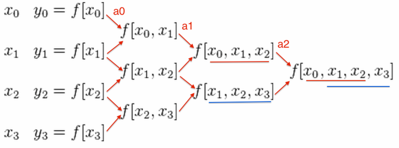
We can calculate the coefficients of Newton polynomial using the following table
![{\displaystyle {\begin{matrix}x_{0}&y_{0}=f[x_{0}]&&&\\&&f[x_{0},x_{1}]&&\\x_{1}&y_{1}=f[x_{1}]&&f[x_{0},x_{1},x_{2}]&\\&&f[x_{1},x_{2}]&&f[x_{0},x_{1},x_{2},x_{3}]\\x_{2}&y_{2}=f[x_{2}]&&f[x_{1},x_{2},x_{3}]&\\&&f[x_{2},x_{3}]&&\\x_{3}&y_{3}=f[x_{3}]&&&\\\end{matrix}}}](https://wikimedia.org/api/rest_v1/media/math/render/svg/4d541beb187dfc9af8782f1a13c8a284937cd8af)
because
![{\displaystyle f[x_{i}]=y_{i}}](https://wikimedia.org/api/rest_v1/media/math/render/svg/155fee5ebbf6543462143a8a14da42bcbb14a0a3)
![{\displaystyle f[x_{i},x_{i+1}]={\frac {f[x_{i+1}]-f[x_{i}]}{x_{i+1}-x_{i}}}}](https://wikimedia.org/api/rest_v1/media/math/render/svg/3abf9e649a77e00375f64531d62502866060bda3)
The following figures shows the dependency between the divided differences:

For example, given data points  ,
,  ,
,  , and
, and  we can draw the following table:
![{\displaystyle {\begin{array}{|c||c|c|c|c|c|}i&x_{i}&y_{i}&f[x_{i},x_{i+1}]&f[x_{i},x_{i+1},x_{i+2}]&f[x_{i},x_{i+1},x_{i+2},x_{i+3}]\\\hline 0&x_{0}=1&{\begin{aligned}y_{0}&=f[x_{0}]\\&=6\end{aligned}}&{\begin{aligned}f[x_{0},x_{1}]&={\frac {f[x_{1}]-f[x_{0}]}{x_{1}-x_{0}}}\\&={\frac {11-6}{2-1}}\\&=5\end{aligned}}&{\begin{aligned}f[x_{0},x_{1},x_{2}]&={\frac {f[x_{1},x_{2}]-f[x_{0},x_{1}]}{x_{2}-x_{0}}}\\&={\frac {7-5}{3-1}}\\&=1\end{aligned}}&{\begin{aligned}&f[x_{0},x_{1},x_{2},x_{3}]\\&={\frac {f[x_{1},x_{2},x_{3}]-f[x_{0},x_{1},x_{2}]}{x_{3}-x_{0}}}\\&={\frac {1-1}{4-1}}\\&=0\end{aligned}}\\\hline 1&x_{1}=2&{\begin{aligned}y_{1}&=f[x_{1}]\\&=11\end{aligned}}&{\begin{aligned}f[x_{1},x_{2}]&={\frac {f[x_{2}]-f[x_{1}]}{x_{2}-x_{1}}}\\&={\frac {18-11}{3-2}}\\&=7\end{aligned}}&{\begin{aligned}f[x_{1},x_{2},x_{3}]&={\frac {f[x_{2},x_{3}]-f[x_{1},x_{2}]}{x_{3}-x_{1}}}\\&={\frac {9-7}{4-2}}\\&=1\end{aligned}}&\\\hline 2&x_{2}=3&{\begin{aligned}y_{2}&=f[x_{2}]\\&=18\end{aligned}}&{\begin{aligned}f[x_{2},x_{3}]&={\frac {f[x_{3}]-f[x_{2}]}{x_{3}-x_{2}}}\\&={\frac {27-18}{4-3}}\\&=9\end{aligned}}&&\\\hline 3&x_{3}=4&{\begin{aligned}y_{3}&=f[x_{3}]\\&=27\end{aligned}}&&&\\\end{array}}}](https://wikimedia.org/api/rest_v1/media/math/render/svg/2b95d23005f4c17a4294dc9c7a8fb4c58e8487ed)
The four data points lie on a polynomial of order 2, which is why the coefficient  (
(![{\displaystyle f[x_{0},x_{1},x_{2},x_{3}]}](https://wikimedia.org/api/rest_v1/media/math/render/svg/22c97723f190624c9bcfaa90c9ace00dfe10311f) ) is zero. Given
) is zero. Given ![{\displaystyle [a_{0},a_{1},a_{2}]=[6,5,1]}](https://wikimedia.org/api/rest_v1/media/math/render/svg/babb93ee773e83c7aa69d6ff6861773eadd11160) the result polynomial is:
the result polynomial is:

Once the coefficients of a Newton's polynomial are solved, we can evaluate the polynomial function for any  . A Newton polynomial is often rewritten in a nested form:
 ,
,
because this nested form of interpolating polynomial is easier to evaluate because x only appears in the function n times.
For example, the nested form of a third order interpolating polynomial is:

The algorithm of Newton's method and its implementation can be found in this Jupyter notebook.
Lagrange polynomial is another form used for polynomial interpolation. It is called a form because with a given set of distinct points the interpolating polynomial is unique. We can arrive at the same polynomial through different methods.
The Lagrange form specifies the interpolation polynomial as:


where  is the order of the polynomial.
For example, given two data points we get  and
and

Obviously the function curve passes both data points. The first derivative also matches that of the divided difference method:

Spline interpolation uses a number of polynomial functions to interpolate a set of data points with each polynomial for two adjacent data points. The Spline method is necessary because often times when the order of the polynomial become large polynomial interpolation shows oscillatory behavior (instability known as Runge's phenomenon). The following iPython notebook shows an example that suffers this issue:
[1]
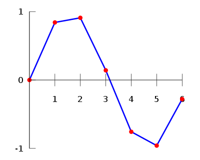
Spline method is not another method for finding polynomial interpolation of a discrete function, but instead it results in a piecewise polynomial (splines) in order to avoid the oscillatory behavior. The most common spline interpolations are linear, quadratic, and cubic splines. Linear interpolation uses lines to connect each pair of consecutive data points resulting in a piecewise interpolation.

A quadratic spline uses a quadratic polynomial to connect consecutive data points.

A function f(x) is a quadratic spline if the following conditions are true:
- The domain of
 is an interval [a, b].
 and
and  are continuous on [a, b].
- The data points
 such that
  and
and  is a polynomial of order at most 2 on each subinterval
 ![{\displaystyle [x_{i},x_{i+1}]}](https://wikimedia.org/api/rest_v1/media/math/render/svg/7138606cdb8eb7dddaba59b5aefe1ade6bc05a1b) .
.


![{\displaystyle f[x_{0},x_{1}]}](https://wikimedia.org/api/rest_v1/media/math/render/svg/a31f8458da9ea4ec290a96134207b45c5d7a4f7c)
![{\displaystyle f(x)=f[x_{0}]+f[x_{0},x_{1}](x-x_{0})+f[x_{0},x_{1},x_{2}](x-x_{0})(x-x_{1})+...}](https://wikimedia.org/api/rest_v1/media/math/render/svg/847c840f35a86400cc5ad569d0be1c07888a60af)
(x-x_{1})(x-x_{2})...(x-x_{n-1})}](https://wikimedia.org/api/rest_v1/media/math/render/svg/58a15892e49e48dcc2f7ed29262bcfb7e0d60634)
![{\displaystyle a_{0}=f[x_{0}]=y_{0}}](https://wikimedia.org/api/rest_v1/media/math/render/svg/b2c02509aa73c0099d52cc8960bd92a2bc3ab880)
![{\displaystyle f[x_{i}]=y_{i}}](https://wikimedia.org/api/rest_v1/media/math/render/svg/155fee5ebbf6543462143a8a14da42bcbb14a0a3)
![{\displaystyle a_{1}=f[x_{0},x_{1}]={\frac {f[x_{1}]-f[x_{0}]}{x_{1}-x_{0}}}}](https://wikimedia.org/api/rest_v1/media/math/render/svg/660a4a2e428dcf77e608eb34d84b1620ff670bbe)
![{\displaystyle a_{2}=f[x_{0},x_{1},x_{2}]={\frac {f[x_{1},x_{2}]-f[x_{0},x_{1}]}{x_{2}-x_{0}}}}](https://wikimedia.org/api/rest_v1/media/math/render/svg/9e5444160c9d00979fb313d269235af8495ed87a)

![{\displaystyle a_{k}=f[x_{0},x_{1},x_{2},\dots ,x_{k-1},x_{k}]={\frac {f[x_{1},x_{2},\dots ,x_{k-1},x_{k}]-f[x_{0},x_{1},x_{2},\dots ,x_{k-1}]}{x_{k}-x_{0}}}}](https://wikimedia.org/api/rest_v1/media/math/render/svg/84da42b61c710539086966d2306a8e67c0986c3f)
![{\displaystyle {\begin{matrix}x_{0}&y_{0}=f[x_{0}]&&&\\&&f[x_{0},x_{1}]&&\\x_{1}&y_{1}=f[x_{1}]&&f[x_{0},x_{1},x_{2}]&\\&&f[x_{1},x_{2}]&&f[x_{0},x_{1},x_{2},x_{3}]\\x_{2}&y_{2}=f[x_{2}]&&f[x_{1},x_{2},x_{3}]&\\&&f[x_{2},x_{3}]&&\\x_{3}&y_{3}=f[x_{3}]&&&\\\end{matrix}}}](https://wikimedia.org/api/rest_v1/media/math/render/svg/4d541beb187dfc9af8782f1a13c8a284937cd8af)
![{\displaystyle f[x_{i},x_{i+1}]={\frac {f[x_{i+1}]-f[x_{i}]}{x_{i+1}-x_{i}}}}](https://wikimedia.org/api/rest_v1/media/math/render/svg/3abf9e649a77e00375f64531d62502866060bda3)


![{\displaystyle {\begin{array}{|c||c|c|c|c|c|}i&x_{i}&y_{i}&f[x_{i},x_{i+1}]&f[x_{i},x_{i+1},x_{i+2}]&f[x_{i},x_{i+1},x_{i+2},x_{i+3}]\\\hline 0&x_{0}=1&{\begin{aligned}y_{0}&=f[x_{0}]\\&=6\end{aligned}}&{\begin{aligned}f[x_{0},x_{1}]&={\frac {f[x_{1}]-f[x_{0}]}{x_{1}-x_{0}}}\\&={\frac {11-6}{2-1}}\\&=5\end{aligned}}&{\begin{aligned}f[x_{0},x_{1},x_{2}]&={\frac {f[x_{1},x_{2}]-f[x_{0},x_{1}]}{x_{2}-x_{0}}}\\&={\frac {7-5}{3-1}}\\&=1\end{aligned}}&{\begin{aligned}&f[x_{0},x_{1},x_{2},x_{3}]\\&={\frac {f[x_{1},x_{2},x_{3}]-f[x_{0},x_{1},x_{2}]}{x_{3}-x_{0}}}\\&={\frac {1-1}{4-1}}\\&=0\end{aligned}}\\\hline 1&x_{1}=2&{\begin{aligned}y_{1}&=f[x_{1}]\\&=11\end{aligned}}&{\begin{aligned}f[x_{1},x_{2}]&={\frac {f[x_{2}]-f[x_{1}]}{x_{2}-x_{1}}}\\&={\frac {18-11}{3-2}}\\&=7\end{aligned}}&{\begin{aligned}f[x_{1},x_{2},x_{3}]&={\frac {f[x_{2},x_{3}]-f[x_{1},x_{2}]}{x_{3}-x_{1}}}\\&={\frac {9-7}{4-2}}\\&=1\end{aligned}}&\\\hline 2&x_{2}=3&{\begin{aligned}y_{2}&=f[x_{2}]\\&=18\end{aligned}}&{\begin{aligned}f[x_{2},x_{3}]&={\frac {f[x_{3}]-f[x_{2}]}{x_{3}-x_{2}}}\\&={\frac {27-18}{4-3}}\\&=9\end{aligned}}&&\\\hline 3&x_{3}=4&{\begin{aligned}y_{3}&=f[x_{3}]\\&=27\end{aligned}}&&&\\\end{array}}}](https://wikimedia.org/api/rest_v1/media/math/render/svg/2b95d23005f4c17a4294dc9c7a8fb4c58e8487ed)

![{\displaystyle f[x_{0},x_{1},x_{2},x_{3}]}](https://wikimedia.org/api/rest_v1/media/math/render/svg/22c97723f190624c9bcfaa90c9ace00dfe10311f)
![{\displaystyle [a_{0},a_{1},a_{2}]=[6,5,1]}](https://wikimedia.org/api/rest_v1/media/math/render/svg/babb93ee773e83c7aa69d6ff6861773eadd11160)


![{\displaystyle [x_{i},x_{i+1}]}](https://wikimedia.org/api/rest_v1/media/math/render/svg/7138606cdb8eb7dddaba59b5aefe1ade6bc05a1b)