High School Trigonometry/Circular Functions of Real Numbers
In this lesson you will view the trigonometric ratios of angles of rotation around the coordinate grid as a continuous, circular function. The connection will be made between how the ratios change as the angle of rotation increases or decreases, and how the graph of the function depicts that change.
Learning Objectives
[edit | edit source]- Identify the 6 basic trigonometric ratios as continuous functions of the angle of rotation around the origin.
- Identify the domain and range of the six basic trigonometric functions.
- Identify the radian and degree measure, as well as the coordinates of points on the unit circle for the quadrant angles, and those with reference angles of 30°, 45°, and 60°.
y = sin(x), The Sine Graph
[edit | edit source]By now, you have become very familiar with the specific values of sine, cosine, and tangents for certain angles of rotation around the coordinate grid. In mathematics, we can often learn a lot by looking at how one quantity changes as we consistently vary another. In this case, what will happen to the value of, let's say, the sine of the angle as we gradually rotate around the coordinate grid. We would be looking at the sine value as a function of the angle of rotation around the coordinate grid. We refer to any such function as a circular function, because they can be defined using the unit circle. First of all, you may recall from earlier sections that the sine of an angle in standard position in the coordinate grid is the ratio of , where y is the y-coordinate of any point on the angle and r is the distance from the origin to that point.


Because the ratios are the same for a given angle, regardless of the length of the radius r, we can use the unit circle to make things a little more convenient.

The denominator is now 1, so we have the simpler expression sin(θ) = y. The advantage to this is that we can use the y-coordinate of the point on the unit circle to trace the value of sin(θ) through a complete rotation. Imagine if we start at 0 and then rotate counter-clockwise through gradually increasing angles. Since the y-coordinate is the sine value, watch the height of the point as you rotate.
Through Quadrant I that height gets larger, starting at 0, increasing quickly at first, then slower until the angle reaches 90°, at which point, the height is at its maximum value, 1.


As you rotate into the third quadrant, the change in the height now reverses itself and starts to decrease towards 0.


When you start to rotate into the third and fourth quadrants, the length of the segment increases, but this time in a negative direction, growing to −1 at 270° and heading back toward 0 at 360°.

After one complete rotation, even though the angle continues to increase, the sine values will simply repeat themselves. The same would have been true if we chose to rotate clockwise to investigate negative angles, and this explains why the sine function is periodic. The period is 2π radians or 360°, because that is the angle measure required before the sine of the angle will simply repeat the previous sequence of values.
Let's translate this circular motion into a graph of the sine value vs. the angle of rotation. The following sequence of pictures demonstrates the connection. As the angle of rotation increases, watch the y-coordinate of the point on the angle as it traces horizontally. Ignore the values along the horizontal axis at this point as they just relative. What is important is that you make the connection between the circular rotation and the change in the height of the point.


Notice that once we rotate around once, the point traces back over the same values again. The red curve that you see is one period of a sine "wave". The below animation shows this happen in "real time".

Let's look at some specific values so we can graph the sine function more precisely. Since we already know what happens in between, you can draw a fairly accurate sketch by plotting the points for the quadrant angles (0, , π, , 2π).


The value of sin(θ) goes from 0 to 1 to 0 to −1 and back to 0. Graphed along a horizontal axis showing θ, it would look like this:

Filling in the gaps in between and allowing for multiple rotations as well as negative angles results in the graph of y = sin(x) where x is any angle of rotation (usually expressed in radians):

As we have already mentioned, sin(x) has a period of 2π. You should also note that the y-values never go above 1 or below −1, so the range of a sine wave is {−1 ≤ y ≤ 1}. Because we can continue to spin around the circle forever, there is no restriction on the angle x, so the domain of sin(x) is all reals.
y = cos(x), The Cosine Graph
[edit | edit source]In chapter 1, you learned that sine and cosine are very closely related. The cosine of an angle is the same as the sine of the complementary angle. So, it should not surprise you that sine and cosine waves are very similar in that they are both periodic with a period of 2π, a range from −1 to 1, and a domain of all real angles.
The cosine of an angle is the ratio of , so in the unit circle, the cosine is the x-coordinate of the point of rotation. If we trace the x−coordinate through a rotation, you will notice the change in the distance is similar to sin(x), but cos(x) starts in a different place. The x−coordinate of a 0° angle is 1 and the x-coordinate for 90° is 0, so the cosine value is decreasing from 1 to 0 through the 1st quadrant.


Here is a similar sequence of rotations to the one we used for sine. This time compare the x coordinate of the point of rotation with the height of the point as it traces along the horizontal.


The graph of y = cos(x) has a period of 2π. Just like sin(x), the x-values never "escape" from the unit circle, so they stay between −1 and 1. The range of a cosine wave is also {−1 ≤ y ≤ 1}. And also just like the sine function, there is no restriction on the angle of rotation, so the domain of cos(x) is all reals.
y = tan(x), The Tangent Graph
[edit | edit source]The graph of the tangent ratio as a function of the angle of rotation presents a few complications. First of all, the domain is no longer all real angles. As you may remember there are some angles (90° and 270°, for example) for which the tangent is not defined. As we will see in this section, the range of tan(x) is actually all real numbers.
The measurement of each of the six trig functions can be found by using a single segment from the unit circle, however, the remaining functions are not as obvious as sine and cosine. The name of the tangent function comes from the tangent line, which is a line that is perpendicular to the radius of a circle at a point on the circle so that the line touches the circle at exactly one, and only one, point. So, to create the tangent segment, first we draw a tangent line perpendicular to the x axis.

If we extend angle θ through the unit circle so that it intersects with the tangent line, the tangent function is defined as the length of the red segment.

The dashed segment is 1 because it is the radius of the unit circle. Recall that the tangent of θ is , so we can verify that this segment is indeed the tangent by using similar triangles.


So, as we increase the angle of rotation, think about how this segment changes. When the angle is 0, the segment has no length. As we begin to rotate through the first quadrant, it will increase, very slowly at first.


But, you can see very soon that the value increases past one. As the angle gets closer to 90°, the segment will need to stretch quite high in order to intersect the extension of the angle and it will grow at a faster and faster rate.


As we get very close to the yaxis that the segment gets infinitely large, until when the angle really hits 90°, at which point the extension of the angle and the tangent line will actually be parallel and therefore never meet!

This means there is no definition for the length of the tangent segment, or as it may be helpful to think of it, the tangent segment is infinitely large.
Before continuing, let's take a look at this portion of the graph through the first quadrant. The tangent starts at 0, for a 0° angle, then increases slowly at first. That increase gets much steeper and as we approach a 90° rotation.
Again, just a small break in the x axis on these graphs will make it more clear that these two concepts to note lie side-by-side on the same coordinate grid.


In fact as we get infinitely close to 90°, the tangent value increases without bound, until when we actually reach 90°, at which point the tangent is undefined. A line that a graph gets infinitely close to without touching is called an asymptote. So the tangent function has an asymptote at 90°.

As we rotate past 90°, now the intersection of the extension of the angle and the tangent line is actually below the x axis. This fits nicely with what we know about the tangent for a 2nd quadrant angle being negative. It will be first be very, very negative, but as the angle rotates, the segment gets shorter, reaches 0, then crosses back into the positive numbers as the angle enters the 3rd quadrant.


The segment will again get infinitely large as it approaches 270°. After being undefined at 270°, the angle crosses into the 4th quadrant and once again changes from being infinitely negative, to approaching zero as we complete a full rotation.

So, this motion graphed over several rotations would look like this:

Notice that the x axis is measured in radians (not in terms of π). Our asymptotes occur every π radians, starting at . The period of the graph is therefore π radians. The domain is all reals except for the "holes" at , , −, etc. and the range is all real numbers.
The Three Reciprocal Functions: cot(x), csc(x), and sec(x)
[edit | edit source]Cotangent
[edit | edit source]Cotangent is the reciprocal of tangent, so it makes sense to generate the circular function for cotangent by drawing the tangent line at a point on the y axis and extending the angle, instead of the x axis.

We can verify that this is the case again by using similar triangles. Because the purported cotangent segment is parallel to the base of the yellow triangle, then angle θ is in the opposite corner and the triangles are indeed similar, even though their positions are reversed.

So,


Now that we have established the cotangent segment, think about how this segment changes as we rotate around the coordinate grid starting at 0°. First of all, at 0° itself, the cotangent is undefined because the segment is parallel to the ray of the angle θ. As we begin to increase the angle of rotation, the segment will be extremely large and begin to get smaller as we approach 90°, very quickly at first, but then slowing down as it gets closer to 0 length at 90°.


After passing 90°, the segment will again start to lengthen, but this time it will be in the negative direction, increasing slowly at first, then getting infinitely large in the negative direction until 180°, at which point it is again undefined.


After passing this point, the periodic behavior kicks in and the function now repeats the same sequence of values as we rotate from 180°, back to 360°.


Tracing this motion on the graph over several rotations gives:

Remember that cotangent and tangent are reciprocals of each other, so any point at which the tangent was equal to 0, the cotangent will be undefined and any point at which the tangent was undefined, the cotangent is equal to 0.

You might also notice that the graphs consistently intersect at 1 and −1. These are the angles that have 45° reference angles, which always have tangents and cotangents equal to 1 or −1. It makes sense that 1 and −1 are the only values for which a function and its reciprocal are the same. Keep this in mind as we look at cosecant and secant compared to their reciprocals of sine and cosine.
The cotangent function has a domain of all real angles except multiples of π {… − 2π. − π.0, π, 2π …} The range is all real numbers.
Cosecant
[edit | edit source]There are many ways possible to find the cosecant segment. One approach is to look at the right triangle formed by the cotangent segment and use the Pythagorean Theorem to generate the cosecant.


From the original triangle in the unit circle, y2 + x2 = r2


Since is cosecant, then the cosecant must be the same as side c.

Tracing the length of this segment, it is undefined at 0°, infinitely large for very small angles, decreasing to 1 at 90° and then increasing infinitely until it is undefined at 180°. The process repeats from 180° to 360°, however, the segment starts infinitely negative, increases to −1 at 270° before approaching an infinitely negative length.


The period of the function is therefore 2π with a domain of all real angles except multiples of π {… −2π, −π, 0, π, 2π …}. The range is all real numbers greater than 1 or less than −1.
The graph then would look as follows:

Here is the graph of y = sin(x) as well:

Notice again the reciprocal relationships at 0 and the asymptotes. Also look at the intersection points of the graphs at 1 and −1. Many students are reminded of parabolas when they look at the half period of the cosecant graph. While they are similar in that they each have a local minimum or maximum and they begin and end in the same direction the comparisons end there and they shouldn't be referred to as parabolic. The mathematics that defines the values, and therefore shape, of the graph is completely different from the quadratic function of a parabola.
Secant
[edit | edit source]Much like the relationship between sine and cosine, secant and cosecant share many similarities. The segment used to generate y = sec(x) is shown below:

You will be asked to demonstrate this in the exercises section. This segment is 1 unit for 0°, then grows through the first quadrant, and is undefined at 90°. It is infinitely negative shrinking down to −1 through the 2nd quadrant, before lengthening back towards infinite negativity and is undefined at 270°. Translating this motion to a graph of y = sec(x) gives us:

Comparing it with the cosine graph:

The period is 2π, the range is the same as y = csc(x) {y : y ≥ 1 or y ≤ −1}, and the domain is all real angles except multiples of {… −, −, , …}.
Lesson Summary
[edit | edit source]The six trigonometric functions defined by the ratios in a right triangle can be placed in the context of the coordinate grid by thinking of them in terms of a point (x, y) rotating around a circle centered at the origin with a radius of one. This circle is called the unit circle. The sine of the angle of rotation is the y−coordinate of the point, the cosine of the angle is the x coordinate, and the tangent is . The values of the other three ratios; cotangent, cosecant, and secant can also be found in terms of their reciprocal relationships, but all of these values can be constructed geometrically as various segments around the angle of rotation on the unit circle. Instead of finding isolated values, we can look at each ratio as a function of the angle of rotation. These are called circular functions. Here are the domains and ranges of the six circular trigonometric functions.
Table 2.3 Function Domain Range sin(x) all reals {y : −1 ≤ y ≤ 1} cos(x) all reals {y : −1 ≤ y ≤ 1} tan(x) {x : x ≠ n · , where n is any odd integer} all reals csc(x) {x : x ≠ nπ, where n is any integer} {y : y > 1 or y < −1} sec(x) {x : x ≠ n · , where n is any odd integer} {y : y > 1 or y < −1} cot(x) {x : x ≠ n · , where n is any odd integer} all reals
Review Questions
[edit | edit source]- Show that side A in this drawing is equal to sec(θ).

- In Chapter 1, you learned that tan2(θ) + 1 = sec2(θ). Use the drawing and results from question 1 to demonstrate this identity.
- This diagram shows a unit circle with all the angles that have reference angles of 30°, 45°, and 60°, as well as the quadrant angles. Label the coordinates of all points on the unit circle. On the smallest circle, label the angles in degrees, and on the middle circle, label the angles in radians.

- Draw and label the line segments in the following drawing that represent the six trigonometric functions (sine, cosine, tangent, cosecant, secant, cotangent).

- Which of the following shows functions that are both increasing as x increases from 0 to ?
- (a) sin(x) and cos(x)
- (b) tan(x) and csc(x)
- (c) sec(x) and cot(x)
- (d) csc(x) and sec(x)
- Which of the following statements are true as x increases from to 2π?
- (a) cos(x) approaches 0
- (b) tan(x) gets infinitely large
- (c) cos(x) < sin(x)
- (d) cot(x) gets infinitely small


Review Answers
[edit | edit source]- Use similar triangles:


So: 
Using the Pythagorean Theorem then, tan2(θ) + 1 = sec2(θ).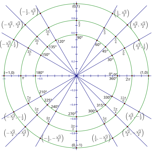

- b
- d


This material was adapted from the original CK-12 book that can be found here. This work is licensed under the Creative Commons Attribution-Share Alike 3.0 United States License