Fractals/Conformal map
Here are examples of conformal maps[1] applied to pictures. This technique is a generalization of domain coloring where the domain space is not colored by a fixed infinite color wheel but by a finite picture tiling the plane. A pedagogical interest is to have a flow of pictures coming from a webcam to allow more interactivity and a richer feedback loop.[2]
Conformal maps
[edit | edit source]

A conformal map is a transformation of the plane preserving angles. The plane can be parametrized by Cartesian coordinates where a point is denoted as , but for conformal maps, it is better to understand it as the complex plane where points are denoted .


In complex coordinates, the multiplication by a real number r corresponds to a homothety, by a unitary number to a rotation of angle θ and by a generic complex number to a similarity mapping.


A holomorphic function is a conformal map because it is locally a similarity with the derivative and the value of f at z0. The derivative is the local zoom factor of the transformation.


After similarities, which have constant derivative function, polynomials and in particular monomials are the simplest holomorphic functions. Its derivative is , it is null at the origin; hence the associated map is conformal only away from the origin.


A problem we face to represent them is that a holomorphic function is in general not injective: Consider the monomial for example, k different points are mapped to the same value.

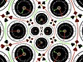
Considering the plane tiled by the picture of the clock, it becomes, when squared the following blurry picture:

We see that the central disk is globally preserved, mapped to itself, but each point (except zero) is covered twice, rendering the picture blurry. For example +1 (at 3 oclock) and −1 (9:00) are both sent to +1 (to the middle right), +i (noon) and i (6:00) are sent to −1 (to the middle left).
In order to get an injective application, we can either restrict ourselves, for example, to the positive real half plane, or to the negative real half plane.


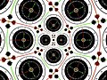
Seen from further away, we get the same big picture for the whole tiling.
-
 The negative real half plane to the square.
 -
 Clock to the square: conformal but not injective.
 -
 The positive real half plane to the square.


Pull-back
[edit | edit source]
To get a nice conformal picture, it is easier and more natural to consider not the direct image but the preimage.
This is exactly how a lot of information of earth is pictured. For example, a map setting to each point a temperature value is pictured by plotting every point of the globe with a color specifying the value of the temperature function at that point. The target space, the temperature space, is painted from blue for small values to red for large values. The same graphing technique is used here but the target space is not 1-real dimensional; it is not a line but the whole plane.
The picture tiles no longer the domain of the application but its target space. The point z colored according to the pixel f(z).


Notice the duplication: points z and −z are colored similarly because they are both mapped to the same image z2.


Likewise, the monomial of order k maps k different points to the same image.
A lot of useful information can be understood concerning the conformal map by picturing its pull-back. Since the forward zoom factor is the derivative, the pull-back zoom factor is the 'inverse' of the derivative. Therefore something very special takes place at the zeros of the derivative of the function, the zoom factor becomes infinite, and it shows. Moreover the degree of the zero can be read by the number of time a feature repeats itself around the singularity. We notice as well when the derivative is real and positive, the picture is "standing up", and when it is real and negative, the picture is "upside-down". When we restrict ourselves to the real axis, we can figure out a sketch of the graph of a real function. We notice as well the inflexion points as a minimum or maximum of the zoom factor.
Inversion, poles
[edit | edit source]After holomorphic functions, locally conformal maps comprise as well meromorphic functions, and the position and order of their poles can be read-off.


The inversion has a simple pole at zero. It is a Möbius transformation with a, b, c and d four complexes such that , therefore it maps circles and lines to circles and lines. In particular horizontals and verticals become circles through zero. Inversion exchanges interior and exterior of the unit disk.


Like zeros, poles can be of higher order than simple. Circles are only infinitesimally preserved in general. We can picture higher order poles as several simple poles coming together.
Logarithm and exponential
[edit | edit source]


A very important map in complex analysis and cartography is the transformation from cartesian coordinates (x,y) to polar coordinates (r,θ). This transformation is realized by the couple of functions logarithm/exponential reciprocal of each other (). Indeed,

maps (r, θ) to (x = log(r), y = θ) and maps (x, y) to (r = exp(x), θ = y).


In picture, the logarithm unwraps circles centered at the origin into vertical lines, and maps rays to horizontal lines. The exponential on the contrary wraps vertical lines into concentric circles, and maps horizontal lines to rays through the origin. Notice that the logarithm goes to infinity at zero, but at a much slower pace than the inversion.
Changing the basis of the lattice, one can obtain spiral variations. As poles and zeros, logarithmic singularities can be added.


Essential singularity
[edit | edit source]

Analytic functions suffer from another type of singularities, for example the essential singularity is zero for , with an accumulation of zeros, and an accumulation of poles for .


Convergence radius
[edit | edit source]Analytic functions are summable in power series. At a given point, its Taylor series admits a convergence radius. Comparison of pull-backs of the function and its truncated Taylor series allows us to illustrate this notion:
-
 The tangent function has a simple pole every kπ/2. It has an essential singularity at infinity.
 -
 Its Taylor series at 0 of order 7 is a good approximation in its disk of convergence.


Programs
[edit | edit source]- zipper by Don Marshall
- ConformalMaps in Julia by Samuel S. Watson
- Numerically Approximating Conformal Maps with the Zipper Algorithm
- A Julia package implementing the zipper algorithm for numerical conformal maps by RoyWiggins
External links
[edit | edit source]- Category:Conformal mappings in wikipedia
- The pictures were deformed using this Java applet; Another version is available for Mac OS X that deforms the video flux from the webcam.
java -d32 -jar ComplexMap.jar. That's great fun. Using Java Tools for Experimental Mathematics library. - Conformal Mapping Module by John H. Mathews
- interactive visualizations of many conformal maps
- Java applets for visualization of conformal maps
- Conformal Maps by Michael Trott, Wolfram Demonstrations Project.
- Java applet by Jürgen Richter-Gebert using Cinderella.
- Conformal Webcam based on Cinderella. Use your webcam to interactively plot the examples on this page using your webcam feed.
- conformal_map by Yue Liu
See also
[edit | edit source]- Analytical Methods for Squaring the Disc
- Moebius transformation