Advanced Inorganic Chemistry/Printable version
| This is the print version of Advanced Inorganic Chemistry You won't see this message or any elements not part of the book's content when you print or preview this page. |
The current, editable version of this book is available in Wikibooks, the open-content textbooks collection, at
https://en.wikibooks.org/wiki/Advanced_Inorganic_Chemistry
Symmetry Elements
Advanced Inorganic Chemistry/Symmetry Elements (1.1)
Symmetry elements of the molecule are geometric entities: an imaginary point, axis or plane in space, which symmetry operations: rotation, reflection or inversion, are performed. [1],[2] Their recognition leads to the application of symmetry to molecular properties and can also be used to predict or explain many of a molecule’s chemical properties. Symmetry elements and symmetry operations are two fundamental concepts in group theory, which is the mathematical description of symmetry properties that describe the structure, bonding, and spectroscopy of molecules.
Contents
  1. Point of symmetry operations
     1.1. Identity, E
     1.2. Proper Rotation, Cn
     1.3. Reflection, σ
     1.4. Inversion, i
     1.5. Improper Rotation, Sn
  2. Point groups
  3. Example: symmetry of benzene
1. Point symmetry operations
Point symmetry of a molecule results when there exists at least one point in space that remains indistinguishable from the original molecule after any symmetry operation is applied. In other words, a rotation, reflection or inversion operations are called symmetry operations if, and only if, the newly arranged molecule is indistinguishable from the original arrangement. There are five kinds of point of symmetry elements that a molecule can possess, thus, there are also five kinds of point of symmetry operations. All symmetry elements in a molecule must share at least one point in common and this point occurs at the center of the molecule.
1.1. Identity, E
Identity operation comes from the German ‘Einheit’ meaning unity. This symmetry element means no change. All molecules have this element.
-
 Figure 1. CFClBrI. A chiral molecule possesses no symmetry but identity operation, E.

1.2. Proper Rotation, Cn
Proper rotation operates with respect to an axis called a symmetry axis (also known as n-fold rotational axis). An axis around which a rotation by 360°/n (or 2π/n) results in an identical molecule before and after the rotation. The axis with the highest n is called the principal axis.
-
 Figure 2. Octahedral structure of SF6. Proper rotations of SF6 are 5C2, 4C3 and 3C4 and we call C4 the principal axis of SF6.

In general, a molecule contains nCn operations such that {Cn1, Cn2, Cn3,…, Cnn-1, Cnn} where Cnn = E. For example, if there exists C5 axis then there exists 5C5 (2C51, 2C52, C55) operations:
- C51 = C54 since the operation results indistinguishable molecule in clockwise and counter-clockwise, respectively.
- C52 = C53 since the operation results indistinguishable molecule in clockwise and counter-clockwise, respectively.
- C55 = E
1.3. Reflection, σ
Reflection operates with respect to a plane called a plane of symmetry (also known as a mirror plane). There exist three types of mirror planes:
- σh – a horizontal mirror plane of a molecule is perpendicular to the primary axis of a molecule.
- σv – a vertical mirror plane of a molecule includes the primary axis of a molecule and passes through the bonds (atoms).
- σd – a dihedral (also known as a diagonal mirror plane) of a molecule includes the primary axis of a molecule while bisecting the angle between two C2 axes that are perpendicular to it. Therefore, ơd does not pass through the bonds (atoms).
NOTE: σd is a special case of a σv.
-
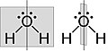 Figure 3. Bent structure of H2O. The water molecule has two σv along C2 axis and no σh.

1.4. Inversion, i
Inversion operates with respect to a point called a center of symmetry (also known as an inversion center). It gives the same result to rotating a molecule around C2 axis then reflecting it with respect to a mirror plane that is perpendicular to C2. For example, SF6 in figure 2 has an inversion point at the center S.
1.5. Improper Rotation, Sn
Improper rotation operates with respect to an axis called rotation-reflection axis. In other words, it is a combination operation of a rotation about an axis by 360°/n (or 2π/n) followed by reflection in a plane perpendicular to the rotation axis.
-
 Figure 4. Staggered ferrocene (left) has an S10 operation while eclipsed ferrocene (right) has an S5 operation.

2. Point groups
The complete collection of symmetry elements of a molecule forms the basis of a mathematical group, and the collection of symmetry operations that are interrelated to each other via certain kind of rules is known as a point group:
- Closure – if any two symmetry operations are in the same group then their product, resulting in another operation, will also be in the same group:
If A∈G and B∈G, then (A∩B)∈G
- Associativity – the law of associativity applies to all symmetry operations:
(AB)C=A(BC)
- Identity – there exists an operation that commutes with other operations (identity, E) and leaves them unchanged:
If A∈G and E∈G, then AE=EA=A
- Inverses – for every symmetry operation in the group, there exists an inverse operation that their product results identity:
If A∈G, then there exists A-1∈G such that AA-1=A-1A=E
For more about mathematical representation of symmetry properties, see also:
- Molecular Point Group (1.2)
- Matrices (1.3)
- Representations (1.4)
in Advanced Inorganic Chemistry.
3. Example: symmetry of benzene
Benzene is one of the molecules that possess various symmetry elements and symmetry operations.

4. References
[1] Pfenning, Brian W. (2015). Principles of Inorganic Chemistry. Hoboken: John Wiley & Sons, Inc.. pp. 195.
[2] https://www-e.openu.ac.il/symmetry/symmetry-tutorial.html
Molecular Point Groups
A Point Group describes all the symmetry operations that can be performed on a molecule that result in a conformation indistinguishable from the original. Point groups are used in Group Theory, the mathematical analysis of groups, to determine properties such as a molecule's molecular orbitals.
Assigning Point Groups
[edit | edit source]While a point group contains all of the symmetry operations that can be performed on a given molecule, it is not necessary to identify all of these operations to determine the molecule's overall point group. Instead, a molecule's point group can be determined by following a set of steps which analyze the presence (or absence) of particular symmetry elements.
- Determine if the molecule is of high or low symmetry.
- If not, find the highest order rotation axis, Cn.
- Determine if the molecule has any C2 axes perpendicular to the principal Cn axis. If so, then there are n such C2 axes, and the molecule is in the D set of point groups. If not, it is in either the C or S set of point groups.
- Determine if the molecule has a horizontal mirror plane (σh) perpendicular to the principal Cn axis. If so, the molecule is either in the Cnh or Dnh set of point groups.
- Determine if the molecule has a vertical mirror plane (σv) containing the principal Cn axis. If so, the molecule is either in the Cnv or Dnd set of point groups. If not, and if the molecule has n perpendicular C2 axes, then it is part of the Dn set of point groups.
- Determine if there is an improper rotation axis, S2n, collinear with the principal Cn axis. If so, the molecule is in the S2n point group. If not, the molecule is in the Cn point group.

The steps for determining a molecule's overall point group are shown in the included flowchart.

Example: Finding the point group of benzene (C6H6)
[edit | edit source]- Benzene is neither high or low symmetry
- Highest order rotation axis: C6
- There are 6 C2 axes perpendicular to the principal axis
- There is a horizontal mirror plane (σh)
Benzene is in the D6h point group.
Low Symmetry Point Groups
[edit | edit source]Low symmetry point groups include the C1, Cs, and Ci groups.
| Group | Description | Example |
|---|---|---|
| C1 | only the identity operation (E) | CHFClBr |
| Cs | only the identity operation (E) and one mirror plane | C2H2ClBr |
| Ci | only the identity operation (E) and a center of inversion (i) | C2H2Cl2Br |
High Symmetry Point Groups
[edit | edit source]High symmetry point groups include the Td, Oh, Ih, C∞v, and D∞h groups. The table below describes their characteristic symmetry operations. The full set of symmetry operations included in the point group is described in the corresponding character table.
| Group | Description | Example |
|---|---|---|
| C∞v | linear molecule with an infinite number of rotation axes and vertical mirror planes (σv) | HBr |
| h | linear molecule with an infinite number of rotation axes, vertical mirror planes (σv), perpendicular C2 axes, a horizontal mirror plane (σh), and an inversion center (i) | CO2 |
| Td | typically have tetrahedral geometry, with 4 C4 axes, 3 C2 axes, 3 S4 axes, and 6 dihedral mirror planes (σd) | CH4 |
| Oh | typically have octahedral geometry, with 3 C4 axes, 4 C3 axes, and an inversion center (i) as characteristic symmetry operations | SF6 |
| Ih | typically have an icosahedral structure, with 6 C5 axes as characteristic symmetry operations | B12H122- |
D Groups
[edit | edit source]The D set of point groups are classified as Dnh, Dnd, or Dn, where n refers to the principal axis of rotation. Overall, the D groups are characterized by the presence of n C2 axes perpendicular to the principal Cn axis. Further classification of a molecule in the D groups depends on the presence of horizontal or vertical/dihedral mirror planes.
| Group | Description | Example |
|---|---|---|
| Dnh | n perpendicular C2 axes, and a horizontal mirror plane (σh) | benzene, C6H6 is D6h |
| Dnd | n perpendicular C2 axes, and a vertical mirror plane (σv) | propadiene, C3H4 is D2d |
| Dn | n perpendicular C2 axes, no mirror planes | [Co(en)3]3+ is D3 |
C Groups
[edit | edit source]The C set of point groups are classified as Cnh, Cnv, or Cn, where n refers to the principal axis of rotation. The C set of groups are characterized by the absence of n C2 axes perpendicular to the principal Cn axis. Further classification of a molecule in the C groups depends on the presence of horizontal or vertical/dihedral mirror planes.
| Group | Description | Example |
|---|---|---|
| Cnh | horizontal mirror plane (σh) perpendicular to the principal Cn axis | boric acid, H3BO3 is C3h |
| Cnv | vertical mirror plane (σv) containing the principal Cn axis | ammonia, NH3 is C3v |
| Cn | no mirror planes | P(C6H5)3 is C3 |
S Groups
[edit | edit source]The S set of point groups are classified as S2n, where n refers to the principal axis of rotation. The S set of groups are characterized by the absence of n C2 axes perpendicular to the principal Cn axis, as well as the absence of horizontal and vertical/dihedral mirror planes. However, there is an improper rotation (or a rotation-reflection) axis collinear with the principal Cn axis.
| Group | Description | Example |
|---|---|---|
| S2n | improper rotation (or a rotation-reflection) axis collinear with the principal Cn axis | 12-crown-4 is S4 |
See Also
[edit | edit source]
Matrix (1.3)
A matrix is a rectangular array of quantities or expressions in rows (m) and columns (n) that is treated as a single entity and manipulated according to particular rules.[1] The dimension of a matrix is denoted by m × n. In inorganic chemistry, molecular symmetry can be modeled by mathematics by using group theory. The internal coordinate system of a molecule may be used to generate a set of matrices, known as a representation, that corresponds to particular symmetry operations.[2] Matrix modeling thus allows for symmetry operations performed on the molecule to be represented in an identical fashion mathematically.
Matrix Operations
[edit | edit source]Addition
[edit | edit source]The sum of two matrices, A and B, is carried out by adding or subtracting the element of one matrix with the corresponding element of another matrix. These operations may only be performed on matrices of identical dimension.
A + B = where i refers to a particular row and j to a particular column.

Example:


Scalar Multiplication
[edit | edit source]Multiplication of a matrix by a scalar, c, multiplies every element within the matrix by the scalar.
cA = c · Ai,j
Example:
c


Matrix Multiplication
[edit | edit source]Matrix multiplication entails computing the dot product of the row of one matrix, A, with the column of another matrix, B. Matrix multiplication is only defined if the number if columns of A, denoted by n, is equal to the number of rows of B, denoted by m. Their product is then the m × n matrix, C. Matrix multiplication entails some mathematical properties. First, it is associative; in other words, (A × B) × C = A × (B × C). Furthermore, matrix multiplication is not commutative; in other words, A × B =/= B × A
Cm×n = Am×c · Bc×n =

Example:

Row Operations
[edit | edit source]There are three kinds of elementary row operations that are used to transform a matrix:
| Type | Definition | Operation |
|---|---|---|
| Row Switching | The swapping of one row with that of another row | |
| Row Addition | The addition of a multiple of one row to another row | |
| Row Multiplication | Multiplication of a row by a scalar, c, with c ≠ 0 | c |


Square Matrices
[edit | edit source]Square matrices are matrices where the number of rows and number of columns are equal, resulting in an n × n matrix.
Identity Matrix
[edit | edit source]The identity matrix, In, is a diagonal matrix which has all elements along the main diagonal equal to 1 and all other elements equal to 0. Multiplication of another matrix by the identity matrix leaves the first unchanged. Moreover, multiplication with the identity matrix is commutative; in other words, A × I = I × A.
Example:
A·I3 =

Trace
[edit | edit source]Only applicable to square matrices, the trace or character, , of a matrix is the sum of its diagonal entries along the main diagonal.

Determinant
[edit | edit source]The determinant of a matrix, denoted det(A), is a real number computed from a square matrix. A non-zero determinant implies matrix invertibility, which further implies that the set of linear equations comprising the matrix has exactly one solution.
For a 2 × 2 matrix, the determinant is computed as follows:
det(A) =

For a 3 × 3 matrix, the determinant is computed as follows:
det(A) =

Higher order determinants may be calculated by using Cramer's Rule.
References
[edit | edit source]- ↑ "Matrix [Def. 3]. In Oxford Dictionaries (American English) (US)". www.oxforddictionaries.com. Retrieved 2016-05-31.
- ↑ Pfenning, Brian W. (2015). Principles of Inorganic Chemistry. Hoboken: John Wiley & Sons, Inc. p. 195. ISBN 9781118859100.
Representations
Representation
[edit | edit source]A representation is a set of matrices, each of which corresponds to a symmetry operation and combine in the same way that the symmetry operators in the group combine.1 Symmetry operators can be presented in matrices, this allows us to understand the relationship between symmetry operators through calculation from matrices. In order to understand representations, knowing matrix notions for symmetry operations is essential.
Here is some examples of symmetry operations in matrix form:
a point in space =

E =

i =

σxy =
Cn = (setting z as the principal axis)

Sn = (setting z as the principal axis)

For Cn operation, θ depends on n with the relationship of θ = . If the symmetry is C2, then θ would be 180° because the molecule is rotated 180°. For C3, θ would be 120°, C4 θ would be 90°, etc.

To apply a symmetry operation on an atom of a molecule, matrices can be combined to produce another operation in the group. For a C2v symmetry compound such as water shown in figure 2, the operations (E, C2, σv1, σv2) can be applied on the vector (x, y, z) to find the representation. To simplify the math, a 1x1 matrix can be done by block diagonalizing for individual vector.
For example,
E(y) = [1] [y] = y
C2(y) = [-1] [y] = -y
σv1(y) = σxz = [-1] [y] = -y
σv2(y) = σyz = [1] [y] = y
In this example, if you apply identity (E) on vector y shown in figure 3, you would obtain y. If you apply C2 rotation along the principal axis on y, then you would obtain -y, etc. These obtained results show the position of the vector after the symmetry operation. The coefficient of each vector after symmetry operation can be represented as Γy in character table shown in figure 1. This set of matrices each of which corresponds to the character of a matrix a representation1. The same symmetry operation can be applied on x and z to obtain a representation for Γx and Γz.

Figure 1. xyz representations in C2v.
_z-axis_b)_y-axis_c)_x-axis.png)
Figure 2. Water molecule a) z-axis b) y-axis c) x-axis

Figure 3. y vector on a cartesian coordinate.
A representation can combine in the same way that the symmetry operators in the group combine, thus, the multiplication table for the matrices that represent each symmetry operation must also multiply together in the same way that the symmetry operators themselves multiply.1 Refer to figure 4.

Figure 4. Multiplication tables for the C2v point group, showing how the 1 × 1 matrix representations multiply together in the same way that the symmetry operations do.
Irreducible Representation and Reducible Representations
[edit | edit source]A representation can be categorized as irreducible representation and reducible representations. A character table is given with irreducible representations, which are the blue shaded part in figure 5. There are 5 rules to irreducible representations, shown in the following.
5 Rules:
1. The sum of the squares of the dimensions of the irreducible representations of a group is equal to the order of the group.
h = Σi li2
2. The sum of the squares of the characters in any irreducible representation equals h.
h = Σi [Xi (R)2]
3. The vectors whose components are the characters of two different irreducible representations are orthogonal.
ΣR [XiR * XjR] = 0, if i =/= j
4. In a given representation (reducible or irreducible) the characters of all matrices belonging to symmetry operations in the same class are identical.
The classes correspond directly to the sets of equivalent operations. Two operations belong to the same class when one may be replaced by the other in a new coordinate system that is accessible by a symmetry operation. For example, a C7 point group would have C71, C72, C73, C74, C75, C76, C77. Since cos(θ) = cos(θ), the characters associated with these matrices are the same. In this case, C71=C76, C72 = C75, C73 = C74, and C77 = E because they belong to the same class. We can simplify the C7 point group’s symmetry into 2 C71, 2C72, 2C73, and E because there are two operations belonging to the same class.
5. The number of irreducible representations of a group is equal to the number of classes in the group.

Figure 5. a) Blue shaded part: irreducible representation b) Green shaded part: reducible representation c) Yellow shaded part: Reducing reducible representations into irreducible representation
The green shaded part in figure 5 is a the reducible representation that is found based on number of unmoved molecule after a symmetry operation. For example, if we are looking at Γσ of C2v symmetry molecule such as water from figure 5, we would focus on the number of unmoved σ bonds after the symmetry operation. In a water molecule, there are two s bonds which are the two O-H bonds. If we apply E, both of the bonds don’t move, so the reducible representation would be 2 because each unmoved σ bonds contribute to 1 reducible representation. If we apply C2 operation on it, both bonds would move, where the O-H bonds would switch places. This means that there are zero unmoved σ bonds, so the reducible representation would be zero as shown in figure 5 b.
The yellow shaded part in figure 5 is the reduction of reducible representations into irreducible representations. This can be done by using the formula, ni = ΣNXRXI, where ni = # of times the irreducible representation occurs in the reducible representation, N = the coefficient in front of each symmetry element symbol (shown on the top row of the character table), h = order of the group (sum of the coefficients N), XR, XI = characters of the reducible and irreducible representations.

Citation
[edit | edit source]1. Pfennig, Brian (2015). Principles of Inorganic Chemistry. Hoboken, New Jersey: John Wiley & Sons, Inc.. pp. 195–202. ISBN 978-1-118-85910-0.
Character Tables
Definition of a Character Table
A character table is a 2 dimensional chart associated with a point group that contains the irreducible representations of each point group along with their corresponding matrix characters. It also contains the Mulliken symbols used to describe the dimensions of the irreducible representations, and the functions for symmetry symbols for the Cartesian coordinates as well as rotations about the Cartesian coordinates.
Components of a Character Table
A character table can be separated into 6 different parts, namely:

| 1. | The Point Group |
| 2. | The Symmetry Operations |
| 3. | The Mulliken Symbols |
| 4. | The Characters for the Irreducible Representations |
| 5. | The Functions for Symmetry Symbols for Cartesian Coordinates and Rotations |
| 6. | The Functions for Symmetry Symbols for Square and Binary Products |
1. The Point Group
The symbol for the point group is found on the uppermost left corner of the character table. It denotes a collection of symmetry operations that are present in a molecule. It is called a point group because all the symmetry elements will intersect at one point[1].
2. The Symmetry Operations/Elements
A symmetry operation is “a geometrical operation that moves an object about some symmetry element in a way that brings the object into an arrangement that is indistinguishable from the original”(Pfennig, 199)[2]. The symmetry operations are at the first row at the top of the table. They are organized into classes, with each class having an order number in front of it. For example, 2S4 represents the operation S4 with order number 2. Operations can belong to the same class when one operation may be replaced by another in a new coordinate system that is accessible by a similar symmetry operation.
Common symmetry operations that are present in character tables are:
| E | Cn | C’n |
| σd | σv | σd |
| I | Sn | C”n |
3. The Mulliken Symbols
These are symbols that occur under the first column of the character table. They are named after Robert S. Mulliken , who suggested using the symbols to describe the irreducible representations. The meanings of the symbols are as follows:
•The dimensions/degeneracy of characters are denoted by the letters A,B,E,T,G and H with each letter representing degeneracy 1,1,2,3,4 and 5 respectively i.e.
| Mulliken Symbol | Number of Dimensions |
|---|---|
| A,B | 1 |
| E | 2 |
| T | 3 |
| G | 4 |
| H | 5 |
For example, the Mulliken symbol A is singly degenerate and symmetric with respect to the rotation about the principal axis whereas the symbol B is anti-symmetric with respect to rotation about the principal axis even though it is also singly degenerate[3].
•The subscripts featured with each Mulliken symbol also represent different aspects of symmetry i.e.
| Subscript / Superscript | Meaning |
|---|---|
| Subscript 1 | symmetric with respect to the Cn principle axis, if no perpendicular axis, then it is with respect to σv |
| Subscript 2 | anti-symmetric with respect to the Cn principle axis, if no perpendicular axis, then it is with respect to σv |
| Subscript g | symmetric with respect to the inverse |
| Subscript u | anti-symmetric with respect to the inverse |
| Superscript prime | symmetric with respect to σh |
| Superscript double prime | anti-symmetric with respect to σh |
4. The Characters for Irreducible Representations[4]
These are the rows of numbers at the center of the character table. They represent the irreducible representations of each Mulliken symbol under the point group. A representation is “a set of matrices, each corresponding to a single operation in the group, which can be combined amongst themselves similarly to how the group elements (symmetry operations) combine” .
These characters correspond to the characters of individual symmetry operations that can be described matrices, themselves. Each character can adopt a +1 or -1 or multiple of this numerical value depending on the symmetric or anti-symmetric behavior of the object undergoing a specific symmetry operation. If the object is symmetric with respect to itself after undergoing the operation, then the character is +1. If the object is anti-symmetric, then the character is -1[5].
5. The Functions for Symmetry Symbols for Cartesian Coordinates and Rotations
These are the symbols that correspond to the symmetry of the Cartesian coordinates (x, y, z) and the symmetry of the rotations about the Cartesian coordinates (Rx, Ry, Rz). They form basis representations for the group and are related to the transformation properties of the group.
For example, for the C3v point group, it can be said that z forms a basis for the A1 representation, x forms a basis for the E representation, and Rz forms a basis for the A2 representation.
6. The Functions for Symmetry Symbols for Square and Binary Products
These are the symbols for the functions that correspond to the square (x2+y2, z2, x2-y2) and binary products (xy, xy, yz) of the Cartesian Coordinates with respect to their transformation properties.
For example, for the C3v point group, it can be said that z2 forms a basis for the A1 representation, (xz,yz) forms a basis for the E representation, and there is no function for the A2 representation.
Mathematics of Character Tables
Each character table follows some main set of mathematical operations that allow for the calculation of important characteristics of the table. These operations are as follows:
a. The order of the group (h) can be calculated by taking the sum of the order of individual symmetry operations in a character table. For example, the order of the C3v point group is 6.
b. The sum of the squares of the dimensions of the irreducible representations of a group is equal to the order of the group.
c. The sum of the squares of the characters in any irreducible representation equals h.
d. The vectors whose components are the characters of two different irreducible representations are orthogonal.
e. In a given representation (reducible or irreducible) the characters of all matrices belonging to symmetry operations in the same class are identical.
f. The number of irreducible representations of a group is equal to the number of classes in the group.
Examples of Character Tables
The Character Table for the C2 Point Group
| C2 | E | C2 | Linear Functions, Rotations | Quadratic Functions | Cubic Functions |
|---|---|---|---|---|---|
| A | +1 | +1 | z, Rz | x2, y2, z2, xy | z3, xyz, y2z, x2z |
| B | +1 | -1 | x, y, Rx, Ry | yz, xz | xz2, yz2, x2y, xy2, x3, y3 |
The Character Table for the Td Point Group
| Td | E | 8C3 | 3C2 | 6S4 | 6σd | Linear Functions, Rotations | Quadratic Functions | Cubic Functions |
|---|---|---|---|---|---|---|---|---|
| A1 | +1 | +1 | +1 | +1 | +1 | - | x2+y2+z2 | xyz |
| A2 | +1 | +1 | +1 | -1 | -1 | - | - | - |
| E | +2 | -1 | +2 | 0 | 0 | - | (2z2-x2-y2, x2-y2) | - |
| T1 | +3 | 0 | -1 | +1 | -1 | (Rx, Ry, Rz) | - | [x(z2-y2), y(z2-x2), z(x2-y2)] |
| T2 | +3 | 0 | -1 | -1 | +1 | x, y, z | xy, xz, yz | (x3, y3, z3), [x(z2+y2), y(z2+x2), z(x2+y2)] |
The Character Table for the D2d Point Group
| D2d | E | 2S4 | C2(z) | 2C'2 | 2σd | Linear Functions, Rotations | Quadratic Functions | Cubic Functions |
|---|---|---|---|---|---|---|---|---|
| A1 | +1 | +1 | +1 | +1 | +1 | - | x2+y2, z2 | xyz |
| A2 | +1 | +1 | +1 | -1 | -1 | Rz | - | z(x2-y2) |
| B1 | +1 | -1 | +1 | +1 | -1 | - | x2-y2 | - |
| B2 | +1 | -1 | +1 | -1 | +1 | z | xy | z3, z(x2+y2) |
| E | +2 | 0 | -2 | 0 | 0 | (x, y),(Rx, Ry) | (xz, yz) | (xz2, yz2),(xy2, x2y),(x3, y3) |
References
SALCs and the projection operator technique
SALCs refers to Symmetry Adapted Linear Combinations, which are generated via use of the projection operator technique. This technique is a mathematical method which outputs a function called a SALC that models the orbitals of the atoms of interest.<ref>[2] These SALCs are mathematical representations and therefore bare no physical meaning. They are commonly used in the generation of molecular orbitals.
Projection Operator Technique
[edit | edit source]The Projection Operator Technique utilizes the extended character table which includes each symmetry operation separately. The technique involves multiple steps, listed below in the form of the BF3 example.
1. We begin by determining the reducible representations of the orbitals in question. For BF3, which has the D3h point group, the D3h character table is used. For our example, we will consider the sigma and pi bonds of the fluorine atoms and determine their reducible representations. Using the character table, we identify the reducible representations. They are listed below.

Γσ = Α1'+ Ε'
Γπx = Α2' + Ε'
Γπy = Α2" + Ε"
Γπz = Α1' + Ε'
It is noted here that the πz orbitals transform as σ orbitals.

2. We now use the extended character table for the D3h Character table to generate the SALCs of the stated orbitals. To do this, we apply each symmetry operation to the given orbital and note which orbital it transforms into. We then add up each projector operator function in accordance to each irreducible representation.
3. Common techniques for dealing with the double degeneracy of the E' and E" representations<ref>[3]:
i. If the principal axis is a C3 axis, we subtract the functions corresponding to the σ2 and σ3 orbitals.
ii. If the principal axis is a C4 axis, we apply the projection operator technique to the σ2 and use the function that is derived.
iii. We must ensure that the representations are orthogonal to one another in order for them to be correct.
4. We can now apply the coefficients within the matrix to determine the coefficients of the function found via the projection operator technique.
We determine the SALCs for the example orbitals to be the following:

SALCσ(A1') = 3σ1 + 3σ2 + 3σ3 = σ1 + σ2 + σ3
SALCσ(E') = 4σ1 - 2σ2 - 2σ3 = 2σ1 - σ2 - σ3
SALCσ(E') = 2σ2 - 2σ3 = σ2 - σ3

SALCπz(A1') = 3π1 + 3π2 + 3π3 = π1 + π2 + π3
SALCπz(E') = 4π1 - 2π2 - 2π3 = 2π1 - π2 - π3
SALCπz(E') = 2π2 - 2π3 = π2 - π3

SALCπx(A2') = 3π1 + 3π2 + 3π3 = π1 + π2 + π3
SALCπx(E') = 4π1 - 2π2 - 2π3 = 2π1 - π2 - π3
SALCπx(E') = 2π2 - 2π3 = π2 - π3

SALCπy(A2") = 3π1 + 3π2 + 3π3 = π1 + π2 + π3
SALCπy(E") = 4π1 - 2π2 - 2π3 = 2π1 - π2 - π3
SALCπy(E") = 2π2 - 2π3 = π2 - π3
Uses of SALCs
[edit | edit source]SALCs help us to understand which orbitals will be bonding, antibonding, and nonbonding. For example, by comparing the symmetry of the SALCs to that of the orbitals of the central atom, it is possible to generate the corresponding molecular orbitals. Although SALCs are mathematical representations that have no physical meaning, they are useful in providing a tool for deriving molecular orbitals.
References
[edit | edit source]1.
- ↑ Johnston, Dean H. "Symmetry @ Otterbein". http://symmetry.otterbein.edu/index.html
- ↑ Pfennig, Brian W. Principles of Inorganic Chemistry. , 2015. Internet resource.
- ↑ “Understanding Character Tables of Symmetry Groups". https://chem.libretexts.org/Core/Physical_and_Theoretical_Chemistry/Group_Theory/Understanding_Character_Tables_of_Symmetry_Groups
- ↑ Rowland, Todd; Weisstein, Eric W. "Character Table". http://mathworld.wolfram.com/CharacterTable.html
- ↑ Jones, Richard. “Character Tables”. University of Texas, Austin. 2015. https://sites.cns.utexas.edu/jones_ch431/character-tables
http://www4.ncsu.edu/~franzen/public_html/CH437/lec8/pdf/projection_1.pdf
2. http://troglerlab.ucsd.edu/GroupTheory224/Chap2B.pdf
Diatomic Molecular Orbitals
The simplicity of diatomic molecular orbitals allows for their inspection using the theory of linear combinations of atomic orbitals (LCAO). As two atoms approach each other, their atomic orbitals overlap. In order to form bonding molecular orbitals, sufficient overlap should occur between atomic orbitals and they must have similar energies and matching symmetries. Anti-bonding molecular orbitals occur when two atomic orbitals cancel each other out. This gives rise to a node or area with zero electron density in between the two atoms.
Molecular Orbitals
[edit | edit source]Just like the atomic orbitals, molecular orbitals(MO) are used to describe the bonding in molecules by applying the group theory. The basic thought of what is molecular orbitals can be the organized combinations of the atomic orbitals according to the symmetry of the molecules and the characteristics of atoms. By applying the MO diagram, the properties such as magnetism and chirality of the molecules can be predicted.
Just like atomic orbitals can be solved as wavefunctions by applying Hermitian Operator to Schrödinger equations, molecule orbitals can be approximated by the linear combinations of atomic orbitals(LCAO):

is the molecular wave function, is the atomic wave functions for atoms, is the adjustable coefficients. This means that when the atoms get closer to each other, their atomic orbitals can overlap and the probability of the occurring of the electrons from the atoms becomes significantly in the overlap regions, which is the formation of the molecular orbitals.


Bonding, Anti-bonding and Non-bonding Molecular Orbitals
[edit | edit source]Before it goes further, some acknowledge about bonding and anti-bonding should be emphasized. When two atomic orbitals overlap, they can form new orbitals in two ways: one is the bonding orbital and another one is the anti-bonding orbital. In a molecular orbital diagram, if atomic orbitals form a bonding orbital, they must form an anti-bonding orbital. The bonding orbitals and anti-bonding orbitals always have the same number and relate with each other. For example, if there is a 1σ bonding orbital, then there must be a 1σ*, which is the relevant anti-bonding orbital of 1σ, where * is used to represent anti-bonding. This bonding and anti-bonding orbitals caused by the different ways of overlapping of the atomic orbitals.
Besides the bonding and anti-bonding molecular orbitals, there can also be some non-bonding orbitals. These orbitals only exist when some atomic orbitals of an atom cannot find any atomic orbital from another atom that has the same symmetry properties, then these atomic orbitals will remain at the same energy and form no bond. That’s why they are called “non-bonding” molecular orbitals.
Diatomic Molecular Orbitals
[edit | edit source]Normally, in diatomic molecular orbitals, the atomic orbitals with the closest energy level can overlap with each other and form molecular orbitals. Therefore, the atomic orbitals generally tend to overlap one by one from the lowest potential energy to the highest potential energy. For example, in a homonuclear diatomic molecule, which means that both atoms are the same element, the same orbitals will overlap together and form molecular orbitals.
Eg. in the oxygen O2, the 1s orbital will overlap with 1s orbital to form a σ orbital and a σ* orbital and the 2s orbital will overlap with 2s orbital to form a σ orbital and a σ* orbital. The 1s orbital cannot overlap with 2s orbital in this case.
For another example, in a heteronuclear diatomic molecule, which means that the atoms in the molecule are different elements, the orbitals with the closest energy can overlap with each other and form molecular orbitals.
Eg. in the hydrogen fluoride HF, hydrogen's 1s orbital will overlap with one of the fluorine's 2p orbitals to form a σ orbital and a σ* orbital since the orbital potential energy of H1s orbital is -13.61eV and of F2p is -18.65eV. Comparing with F2s orbital which has -40.17eV as its orbital potential energy, they are really close to each other. That's why H1s will form molecular orbitals with F2p instead of F2s.[1]
Also notice that only two atomic orbitals with similar symmetry properties can combine together. For example, s orbital can’t overlap with px orbital if the overlap equally with both the same and opposite signs, this will cancel the bonding and anti-bonding effect which will result in no molecular orbital forms.
Besides that, we normally only consider the valence atomic orbitals. That's why the F1s orbital does not be considered here since it's full-filled.
MO from s Orbitals
[edit | edit source]The overlap of two s orbitals will form a σ orbital and a σ* orbital.

MO from p Orbitals
[edit | edit source]The overlap of two p orbitals will form either a σ and a σ* orbitals or a π and a π*orbitals. Generally, we choose to assign the z axis of two atoms point to each other which allows the pz orbitals overlap “head” to “head” and form σ and σ* orbitals. This also allows the px orbitals overlap “side” to “side” and form π and π*orbitals. This also applies for the py orbitals.

Sometimes, when p orbitals can’t find another orbital has a similar symmetry with it, these p orbitals will remain as non-bonding orbitals.

MO from d Orbitals
[edit | edit source]Start from the third row, all the elements after sodium (Na) have d orbitals. There are totally 5 d orbitals, which are named as dz2,dxy,dxz,dyz and dx2-y2. Elements with d orbitals, especially the transition metals, can also form bonds by using d orbitals. As shown in figure 4, the different overlap of the d orbitals will result in different electron density, which results in different types of bonds. Just like what happens to the p-orbital-overlapping molecular orbitals, d atomic orbitals can also overlap with other orbitals in different orbital potential energy levels such as p orbitals and s orbitals. This is also the reason for the formation of a metal complex. However, d orbitals normally are not applied to form molecular orbitals in a diatomic molecule.
Nonbonding Orbitals
[edit | edit source]As mentioned before, if an atomic orbital cannot find any other orbital with similar symmetry, then it will remain as non-bonding molecular orbital. The non-bonding molecular orbitals normally have the same energies as the atomic orbitals that form them, although there are some special cases can happen (not in diatomic MO, but in some metal complex). For example, in the ion FHF-, by solving the irreducible representation, it can be found that the base of FHF- has ag, b2u, b3u, b2g, b3g and b1u. However, since the H atom has only a 1s orbital, it can only form molecular orbitals with ag. Therefore, b2u, b3u, b2g, b3g and b1u will remain as non-bonding molecular orbitals. Also, notice that b1u has a higher level in energy state. This can be caused by the extreme unsymmetrical structure of this molecular orbital. Another guess of the increase in the b1u energy level can be the slightly mixing with the 2s orbital from two fluorines.

Homonuclear Diatomic Molecule
[edit | edit source]Homonuclear diatomic molecules mean that both atoms in the molecules are the same elements. This diatomic molecular type is very simple. By drawing the MO diagram, the existence of the molecules and the magnetic properties can be predicted.
For example, the Lewis structure of O2 predicts that oxygen molecule is a diamagnetic molecule. However, by experiment, O2 liquid is paramagnetic. According to the MO diagram of O2, it has two simple electrons in the * orbitals, which can predict that O2 is actually paramagnetic.

Bond order
[edit | edit source]Bond order can tell us the number of the bond in the molecules. The bond order can be calculated by the equation:

Normally, we only count the valence electrons here since all the orbitals below the valence molecular orbitals are full-filled, which means the number of electrons in bonding orbitals and in anti-bonding orbitals will cancel each other. For example, the bond order of O2 is:

This means that O2 will have 2 bonds, which matches with reality. This method can also be applied to any other diatomic molecules.

Orbital Mixing
[edit | edit source]This is the most tricky part for the diatomic molecular orbitals. In general, we only consider the interactions between atomic orbitals have the same energies unless there is no atomic orbital satisfy the request. However, the interaction between two atomic orbitals with relatively close energies that have the same symmetry can also happen. This will result in the raising of the energies of the molecular orbitals.
Considering figure 2 above, this is an example without interaction between two atomic orbitals with close energies that have the same symmetry. The molecular orbitals have higher energy than the molecular orbital. However, since the and orbitals both have symmetry,these orbitals can interat to lower the energy of the and to increase the energy of the . This will result the energy of orbital has higher energy than orbitals, as shown in figure 7. This phenomenon is called mixing.


For example, this s-p mixing will happen for B2 and C2.
Heteronuclear Diatomic Molecule
[edit | edit source]Unlike the homonuclear diatomic molecule, many heteronuclear diatomic molecules are polar molecules. This means that the electron density does not evenly distribute over each atom. The electron density always favors the atom that is more electronegative. MO theory can also be applied in this situation.
As mentioned before, since here we deal with different two elements in molecules, the orbital potential energies will be considered. This will result in uneven contributions of molecular orbitals from the overlap of the atomic orbitals. Fortunately, farther the two atomic potential energies (APE) are, less the magnitude of the interaction between them. This means that only two atomic orbitals with similar energies can overlap enough to form molecular orbitals. Use the example of HF (Figure 3). According to Table 1, 1s orbital of the hydrogen atom has APE as -13.61eV, 2s orbital of fluorine has APE as -40.17eV and 2p orbitals of fluorine have APE as -18.65eV. It is obvious that orbital has a much closer potential energy to the instead of . Therefore, orbital overlaps much more with and form molecular orbitals. will remain as a non-bonding orbital.


Drawing Diatomic MO Diagram
[edit | edit source]Here are some common steps to help you draw the diatomic MO diagram.
- Recognize the diatomic molecule is a homonuclear molecule or heteronuclear molecule;
- Recognize the orbital potential energies of their valence atomic orbitals, find the closest pair;
- Recognize the symmetry of these atomic orbitals to figure out if the interaction can actually happen. Then determine the and bonding and anti-bonding, and even non-bonding orbitals;
- Recognize the mixing effect to see if there are any energy shift for the molecular orbitals;
- Draw the electrons from the lowest molecular orbital. Follow the rules like the Pauli exclusion principle to draw the ground state MO diagram.

Reference
[edit | edit source]- Miessler, Gary. “Chapter 5. Molecular Orbital Theory.” Inorganic Chemistry, by Gary L. Miessler et al., Pearson, 2014, pp. 117–138.
NH3 Molecular Orbitals
Point Group of NH3
[edit | edit source]
The symmetry elements of NH3 are E, 2C3, and 3 sigma-v. To elaborate, the molecule is of C3v symmetry with a C3 principal axis of rotation and 3 vertical planes of symmetry. The image of the ammonia molecule (NH3) is depicted in Figure 1 and the following character table is displayed below [2]:
| C3v | E | 2C3v | 3 σv | ||
|---|---|---|---|---|---|
| A1 | 1 | 1 | 1 | z | x2+y2, z2 |
| A2 | 1 | 1 | -1 | Rz | |
| E | 2 | -1 | 0 | (x,y)(Rx,Ry) | (x2-y2,xy)(xz,yz) |
The Construction of Molecular Orbitals of NH3
[edit | edit source]The Molecular Orbital Theory (MO) is used to predict the electronic structure of a molecule. Molecular orbitals are formed from the interaction of 2 or more atomic orbitals, and the interactions between atomic orbitals can be bonding, anti-bonding, or non-bonding. A bonding orbital is the interaction of two atomic/group orbitals in phase while an anti-bonding orbital is formed by out-of-phase combinations.
In general, the energy level of molecular orbitals increases from bonding, to non-bonding, and anti-bonding molecular orbitals. Pi-bonding molecular orbitals generally have greater energies than sigma-bonding molecular orbitals because the pi interactions are less effective than sigma interactions. The energy of molecular orbitals increases when the number of nodes also increases, and vice versa [6]. Within bonding molecular orbitals of the same symmetry, the lowest energy are from completely symmetrical sigma bonding molecular orbitals.
Projection Operator Methode:
[edit | edit source]The Projection Operator Methode can be used to determine MO of NH3, the next steps can be used:
1) Determine the point group of molecular;
2) Label S orbital of H;
3) Generate a reducible representation (ᒥ) for H;
4) Reduce reducible representation to irreducible representation;
5) Generate the symmetry adapted linear combinations (SALCs) of orbitals that arise from these irreducible representations;
6) Drawing group orbital combinations and determine the atomic orbitals of the centeral atom;
7) MO
Example
[edit | edit source]
To proceed in constructing the molecular orbitals of NH3, one must first identify the symmetry adapted linear combinations (SALCs) of the 3 hydrogen 1s orbitals. This concept is depicted in Figure 2.
The reduced reducible representation (methodology and concepts further elaborated in Representations section of Advanced Inorganic Chemistry) of the sigma bonds is then written into linear combinations of irreducible representations of ΓSH= a1 + e, as shown in the table. The irreducible representations are determined by the equation ni = 1/h Σ NXRXI where ni is the coefficient of the ith reducible representation, XR and XI are characters of reducible and irreducible representations respectively, N is the coefficient in front of each symmetry elements found on the top row of the character table, and h is the order of the group and sum of the coefficients of the symmetry element symbols.
| C3v | E | 2C3 | 3 σv |
|---|---|---|---|
| A1 | 1 | 1 | 1 |
| A2 | 1 | 1 | -1 |
| E | 2 | -1 | 0 |
| ΓSH | 3 | 0 | 1 |
From the a1 and e symmetry adapted linear combinations, the properties of transformation of the H orbitals are retained in rotational C3 subgroup and so, the C3 is then dropped as shown below:
| C3v | E | C3 | C32 | σv | σv2 | σv3 |
|---|---|---|---|---|---|---|
| S1 | S1 | S2 | S3 | S1 | S3 | S2 |
Under σv's, S1-S3 are already accounted for in the rotation operators.
The applications and concepts of Symmetry Adapted Linear Combinations (SALCs), using projection operators can be found in SALCs and the projection operator technique section in Advanced Inorganic Chemistry. The ligands in Figure 2 are labeled σ1, σ2, and σ3 for S1, S2, and S3, and the normalized SALCs of the sigma orbitals of the ligand groups (Figure 3) can be determined from ΓSH= a1 + e:

| C3v | E | C3 | C32 | σv | σv2 | σv3 |
|---|---|---|---|---|---|---|
| S1 | S1 | S2 | S3 | S1 | S3 | S2 |
From the table above and character table, the irreducible representation found (a1 and e) is taken and the SALCs of the respective ligands are derived:
1. SALC(A1)S1 = S1 + S2 + S3 + S1 + S2 + S3
2. SALC(E)S1 = 2S1 - S2 - S3
3. SALC(E)S2 = -S1 + 2S2 - S3
4. SALC(E)S3 = -S1 - S2 + 2S3
Line A below is obtained by summing up S1, S2, S3 of Line 1, resulting in 2S1 + 2S2 + 2S3. Then, 2S1 + 2S2 + 2S3 was reduced by 2 to give S1 + S2 + S3. Line C below is achieved by subtracting line 3 from line 4, resulting in 0 + 3S2 - 3S3 before reducing it be 3 to give S2 - S3.
A. SALC(A1)S1 = 2S1 + 2S2 + 2S3 ≈ S1 + S2 + S3
B. SALC(E)S1 = 2S1 - S2 - S3
C. SALC(E)S2 - S3 = 3S2 - 3S3 ≈ S2 - S3
The projection operator method is useful in visualizing group orbitals, as shown in Figure 4.

NH3 MO Diagram
[edit | edit source]Molecular orbital diagram is useful in displaying and explaining the chemical bonds of molecules in conjunction with the molecular orbital theory. Formation of molecular orbitals involve interactions between atomic orbitals if their symmetries are compatible with each other, based on group theory. Linear combination of atomic orbitals can only occur with orbitals of similar symmetry. The overlapping orbitals of similar symmetry contributes to the construction of molecular orbitals. When there is a big enough overlap, splitting of the resulting molecular orbitals occurs.
In regards to NH3, the a1 SALC of the 3 H(1s) orbitals can only merge with a1 orbitals of nitrogen (such as the 2s and 2pz). The 2py nitrogen orbital can combine with the e1 SALC and 2px is merged with e2. The linear combination of atomic orbitals is drawn and detailed in Figure 4.

Ammonia or NH3 has 8 valence electrons, consisting of a lone pair on its nitrogen and 3 N-H sigma bonds. The molecular orbital diagram of NH3 is presented in Figure 5 and will be elaborated in regards to its interactions. The s orbitals for the 3 hydrogens are used to set up the sigma and anti bonding combinations of N sp3 orbitals and the H 1s orbitals.
The H3 1s orbitals form an a1 and e combination. Bonding and anti-bonding interactions are made with N orbitals of similar symmetry. The a1 orbital that remained on N is higher in energy above the level of atomic orbital as the orbital interacts with a lower energy a1 bonding orbital. Thus, this orbital is considered non-bonding.

To take note, the a molecular orbitals are non-degenerate and symmetrical with respect to the rotation around z in an x, y, z axis. However, the bonding e orbitals are doubly degenerate orbitals of px and py as shown in Figure 6 [4].
The two frontier molecular orbitals of concern are the highest occupied molecular orbital (HOMO) and lowest unoccupied molecular orbital (LUMO). Taking a look at the molecular orbital diagram of NH3, note that there are 2 electrons in the 2a1 orbital, making it the HOMO. On the other hand, the 3a1 is an anti-bonding molecular orbital and contains no electrons, making it the LUMO. Thus, these 2 orbitals are at the frontiers of the NH3 molecule [1].
In essence, it is valuable to understand and know what molecular orbitals are in terms of their structure, shape, and relative energies because they will ultimately determine the chemistry of the molecule. This helps chemists study and see how a molecule of interest, such as ammonia, reacts.
References
1. Adapted Linear Combinations. Chemistry LibreTexts. National Science Foundation. Sep. 02, 2017. https://chem.libretexts.org/Core/Physical_and_Theoretical_Chemistry/Spectroscopy/Vibrational_Spectroscopy/Vibrational_Modes/Symmetry_Adapted_Linear_Combinations
2. Greeves, N. SALC Ammonia - Molecular Orbitals. ChemTube3D. University of Liverpool. http://www.chemtube3d.com/SALC-ammonia-MO.htm
3. Raj, G.; Bhagi, A.; Jain, V. Group Theory and Symmetry in Chemistry, 3rd ed.; Satyendra Rastogi, 2010. pp 113-114. https://books.google.com/books?id=mTe07xK9f5gC&dq=Group+Theory+and+Symmetry+in+Chemistry,+3rd+ed.%3B+Satyendra+Rastogi&source=gbs_navlinks_s
4. Locke, W. Introduction to Molecular Orbital Theory. ICSTM Department of Chemistry. 1996-1997. http://www.ch.ic.ac.uk/vchemlib/course/mo_theory/
5. SALCS for Common Geometry. The State University of New York. 2018. http://employees.oneonta.edu/viningwj/chem342/SigmaMOdiagramsforTMs.pdf
6. James. The Pi Molecular Orbitals of Benzene. Master Organic Chemistry. 2018. https://www.masterorganicchemistry.com/2017/05/05/the-pi-molecular-orbitals-of-benzene/
Td Molecular Orbitals
Td Point Group
[edit | edit source]The Td symmetry group is a one of the point groups considered to have higher symmetry. Molecules in the Td group, such as methane (CH4) have four C3 rotational axes.
The character table for the Td point group is shown below:
| Td | E | 8C3 | 3C2 | 6S4 | 6σd | ||
|---|---|---|---|---|---|---|---|
| A1 | 1 | 1 | 1 | 1 | 1 | x2+y2+z2 | |
| A2 | 1 | 1 | 1 | −1 | −1 | ||
| E | 2 | −1 | 2 | 0 | 0 | (2z2−x2−y2, x2−y2) | |
| T1 | 3 | 0 | −1 | 1 | −1 | (Rx, Ry, Rz) | |
| T2 | 3 | 0 | −1 | −1 | 1 | (x, y, z) | (xy, xz, yz) |
Constructing Molecular Orbitals
[edit | edit source]Determining Reducible Representations
[edit | edit source]
The first step to constructing the molecular orbitals (MOs) is to determine the reducible representations for the σ and π bond vectors, denoted and , respectively. The character corresponding to each symmetry operation can be determined by tracking how the bond vectors transform. Each vector that is left unmoved will contribute +1, each vector that is shifted to a new position will contribute 0, and each vector that undergoes a sign reversal will contribute −1. The reducible representations and are listed below:


| Td | E | 8C3 | 3C2 | 6S4 | 6σd |
|---|---|---|---|---|---|
| 4 | 1 | 0 | 0 | 2 | |
| 8 | −1 | 0 | 0 | 0 |
Reducing the Reducible Representations
[edit | edit source]The reducible representations obtained from the previous section can be written as linear combinations of the irreducible representations shown in the character table. The contribution of each irreducible representation to the reducible representation is given by the formula

where is the coefficient of the ith reducible representation, is the order of the point group, is the number of symmetry operations in the class, is the character of the reducible representation corresponding to the class, is the character of the irreducible representation corresponding to the class, and the summation is taken over all classes of symmetry operations. Applying this method to the and representations gives


Determining SALCs of Pendant Ligands
[edit | edit source]The Symmetry Adapted Linear Combinations (SALCs) can be found using the projection operator technique. For example, suppose we using the following labelling scheme for the ligand groups in Figure 1: (1) top-left-front, (2) top-right-back, (3) bottom-right-front, (4) bottom-left-back. Then the normalized SALCs for the s orbitals of the ligand groups are


The purpose of using the projection operator method is to be able to draw the SALCs.
Drawing the Molecular Orbital Diagram
[edit | edit source]
Consider CH4 as a specific example of a molecule within the Td symmetry group. Before drawing the MO diagram, the valence atomic orbitals on the central atom and their symmetries must be noted. The symmetry of the orbitals can be determined by determining how they transform under the symmetry operations or by simply looking at the right most columns on the character table. The valence orbitals of the carbon atom include 2s (A1 symmetry) and 2px, 2py, 2pz (T2 symmetry).
In CH4, the only potentially bonding orbitals of the ligand groups are the 1s orbitals in the hydrogen atom. The irreducible representations contributing to the symmetry of the ligand group SALCs determines the AOs of the central atom with which they can interact. As found previously, the SALCs of the hydrogen atoms have A1 + T2 symmetry, so they can interact with all of the valence orbitals on the carbon atom to form bonding and antibonding MOs. Bonding MOs are positive linear combinations of the central atom AOs and ligand group SALCs, while antibonding MOs are negative linear combinations. The number of bonding and antibonding MOs created must be equal to the number of AOs and ligand group orbitals used to create them.
Although in CH4, all AOs and SALCs formed bonding and antibonding MOs, this is not always the case. For example, if a central atom AO has symmetry that is absent from the ligand group SALCs, it will be unable to participate in the formation of bonding and antibonding MOs. In such cases, non-bonding MOs are formed.
The relative energy of the MOs are influenced by a few trends. For MOs formed with similar AOs, the following tend to be true:
- Bonding MOs have lower energy than antibonding MOs. Non-bonding MOs tend to have energy intermediate between bonding and antibonding MOs.
- π bonding MOs have higher energy than σ bonding MOs.
- The energy of MOs increases with the number of nodes.
- The totally symmetric σ bonding MO has the lowest energy among σ bonding MOs.
Illustrations of CH4 MOs can be found in Pfennig's text, Principles of Inorganic Chemistry, pp. 300.
D4h Molecular Orbitals
The D4h point group are one of the most common molecular symmetry found in nature. For example, the XeF4 molecule belongs to the D4h point group. the XeF4 contains one C4 rotation axis, one C2 rotation axis, and four C2 perpendicular rotation axis, 2σv planes, 2σd planes and 1σh plane, those composed the character table of the D4h Point group.
.jpg)
To compose a Molecular Diagram of a molecule with D4h symmetry group, we should first find the irreducible representation of the ligands and of the center molecule. and then find the SALCS for each of the irreducible representation and finally, compose the molecular diagram.
To take an easy example, the Square Planar Complexes..
starting with the sigma orbital of the ligands, the reducible representation of the sigma orbital is the total number of atoms that do not move under each operation. For the Pi orbital, we have to degenerate the pi orbital has two degrees of freedom, thus, the reducible representation of the pi orbital can also be found by using the similar method.
and then, by using the projection operation method, we can find the irreducible representations of the ligand's sigma and pi orbital. In this case, the sigma orbital has A1g, B1g, Eu three irreducible representations and the pi orbital has A2g, A2u, B2g, B2u, Eg and Eu.
| E | 2C4 | C2 | 2C’2 | 2C’’2 | i | 2S4 | σh | 2σv | 2σd | |
|---|---|---|---|---|---|---|---|---|---|---|
| sigma | 4 | 0 | 0 | 2 | 0 | 0 | 0 | 4 | 2 | 0 |
| Pi | 8 | 0 | 0 | -4 | 0 | 0 | 0 | 0 | 0 | 0 |
Move on the central atom, we can find irreducible representation of the valence orbitals on the central atoms by using the character table. The results are as follow:
| Representation | Orbital |
|---|---|
| A1g | s, dz2 |
| B1g | dx2- y2 |
| B2g | dxy |
| Eg | dxz, dyz |
| A2u | Pz |
| Eu | Px, py |

Pi Donor and Acceptor Ligands

The nature of ligands coordinated to the center metal is an important feature of a complex compound along with other properties such as metal identify and its oxidation state. More specifically, it is the identity and consequently the ability of the ligand to donate or accept electrons to the center atom that will determine the molecular orbitals.
The spectrochemical series shows the trend of compounds as weak field to strong field ligands. Furthermore, ligands can be characterized by their π-bonding interactions. This interaction reveals the amount of split between eg and t2g energy levels of the molecular orbitals that ultimately dictates the strength of field of the ligands.
Examples of Weak Field Ligands X-, OH-, H2O ; Examples of Strong Field Ligands H-, NH3, CO, PR3

In a π-donor ligand, the SALCs of the ligands are occupied, hence it donates the electrons to the molecular σ σ* and π π* orbitals. The orbitals associated to eg are not involved in π interactions therefore it stays in the same energy level (figure 1). On the other hand, the occupied ligand SALC t2g orbitals that would form molecular orbitals with the metal t2g orbitals (ie. dxy, dxz, dyz) are lower in energy than its metal counterparts. The resulting MO has π* orbitals that are energetically lower than the σ* orbitals that are formed from the non bonding orbitals (eg). The difference between the t2g π* and eg σ orbitals is denoted as Δ, split. In the π-donor case, the Δ is small due to the low π* level.
Conversely, the t2g SALCs of a pi accepting orbitals are higher in energy than the metal t2g orbitals because they are unoccupied. The resulting t2g π* orbitals are higher than the σ* orbitals. This creates a larger Δ between the eg and t2g π orbitals, making these π-accepting orbitals high split ligands.
Finally, the magnitude of Δ as influenced by the identify of the ligand will dictate how electrons are distributed in the metal d orbitals (figure 2). Weak field ligands produce a small Δ hence a high spin configuration. Strong field ligands produce a large Δ hence a low spin configuration on the d electrons.
Normal Modes of Vibration
Molecular vibrations
[edit | edit source]Molecular vibrations are one of three kinds of motion, occurs when atoms in a molecule are in periodic motion. Molecular vibrations include constant translational and rotational motion. Translational motion occurs when the whole molecule goes in the same direction while the rotational motion occurs when the molecule spins like a top. Molecule vibrations fall into two main categories of stretching and bending. Stretching changes in interatomic distance along bond axis, while bending changes in angle between two bonds in a molecule.
There are two types of stretching, symmetric stretching and asymmetric stretching as the following figure shows:
There are four types of bend, rocking, scissoring, wagging, and twisting:
Normal modes of vibration
[edit | edit source]Each atom in a molecule has three degree of freedom. A molecule with n atoms has 3n degree of freedom. 3n degree of freedom composes of translation, rotations and vibrations. All 3n degrees of freedom have symmetry relationships consistent with the irreducible representations of the molecule's point groups. Non-vibration modes (NVM) include translations and rotations. The vibrational motions of the atoms in a molecule can always be resolved into fundamental vibrational modes for the entire molecule.
Atomic displacement coordinates
[edit | edit source]The number of normal modes of vibration:
- 3n-6 for non-linear molecules
- 3n-5 for linear molecules
To indicate the the number of normal modes of vibration:
- Locate a set of three vectors along the Cartesian coordinates at each atom, representing the 3n degrees of freedom
- Find the reducible representation
- Reduce it to irreducible representations, subtract rotations and translations
- The rest of irreducible representations will give the symmetry of the NMVs
Samples
[edit | edit source]vibrations for SO2
[edit | edit source]| C2v | E | C2 | σv(xz) | σ’v(yz) | ||
|---|---|---|---|---|---|---|
| A1 | 1 | 1 | 1 | 1 | z | x2, y2, z2 |
| A2 | 1 | 1 | -1 | -1 | Rz | xy |
| B1 | 1 | -1 | 1 | -1 | x, Ry | xz |
| B2 | 1 | -1 | -1 | 1 | y, Rx | yz |
| Γ3n | 9 | -1 | 1 | 3 | ||
| Ni | 3 | 1 | 1 | 3 | ||
| Xi | 3 | -1 | 1 | 1 |
Reduce
Γ3n=3A1+A2+2B1+3B2
Γtrans=A1+B1+B2
Γrotations=A2+B1+B2
ΓNMV=Γ3n-6=2A1+B2
NMVs are also identified by frequency numbers: v1, v2, v3,... The numbering is often assigned systematically in descending order of the symmetry species and among modes of the same symmetry in descending order of the vibrational frequency. Stretching modes have higher frequency than bending modes.
Selection Rules for IR and Raman Spectroscopy
Infrared Spectroscopy
Infrared spectroscopy measures the frequency of absorption when a sample is irradiated with infrared electromagnetic radiation. It is a technique used to study the vibrations between atoms because atomic vibrational excitations occur in the infrared region of the electromagnetic spectrum. The bonds between atoms can be thought of as a spring connecting two masses. In the spring-mass analogy the moving system can be approximated by a simple harmonic oscillator. The frequency oscillation is proportional to ,where k is the spring constant and m is the mass of the object. In a similar approximation, the frequency of vibration between two atoms is unique and varies depending on the strength of the bond (k) and the size of the atoms (m). When the frequency of electromagnetic radiation matches the natural frequency of vibration between atoms, the atoms are able to absorb this energy and exhibit vibrations. These vibrations can be detected as signals if they produce a change in the dipole moment between two atoms which can interact with the electric field. Representations for normal modes of vibration will be active in the infrared if they transform similar to any one of the cartesian coordinates (x,y,z). This would mean the vibrational motion has shifted the charge distribution in any of the x, y, or z directions resulting in a change in the dipole moment. Selection rules such as these are used to tell us whether such transitions are allowed, and therefore observed, or whether they are forbidden.

Raman Spectroscopy
Unlike IR spectroscopy which measures the energy absorbed, Raman spectroscopy consists of exposing a sample to high energy monochromatic light that interacts with the molecule and causes electronic, vibrational, or translational excitations. Upon interaction, the energy of the light is shifted either up or down and these changes can give information about the molecule’s various vibrational states. A photon of light excites the molecule to an excited state and upon relaxation to a different rotational or vibrational state the molecule emits a photon of a different energy. A vibration will give rise to a Raman shift, due to a shift from the incident light, if it has the same symmetry as the molecular polarizability. Polarizability measures the ability for a molecule’s electron cloud to become distorted. A dense electron cloud is more difficult to change than a more spread out electron density. The representation for one of the normal modes of vibration will be Raman active if it transforms similarly to the direct products of any one of the x, y, or z coordinates. That includes any of the functions: xy, xz, yz, x2, y2, z2, or any combination.
Rule of Mutual Exclusion
A molecule is centrosymmetric if it has a center of inversion and their corresponding point group contains the class for inversion. In such cases, the unit vectors transform as ungerade, or unsymmetric about the center of inversion, and direct products transform as gerade, or symmetric about the center of inversion. As a result, the normal modes of vibrational will show frequencies in either the IR or Raman, but the same frequency will not be observed in both.
Example Boron Trifluoride or D3d point group
Character Table for D3d:
| D3d | E | 2C3(z) | 3C'2 | σh (xy) | 2S3 | 3σv | Linear Functions/ Rotations | Quadratic Functions | Cubic Functions |
|---|---|---|---|---|---|---|---|---|---|
| A'1 | +1 | +1 | +1 | +1 | +1 | +1 | - | x2+y2, z2 | x(x2-3y2) |
| A'2 | +1 | +1 | -1 | +1 | +1 | -1 | Rz | - | y(3x2-y2) |
| E' | +2 | -1 | 0 | +2 | -1 | 0 | (x,y) | (x2-y2, xy) | (xz2, yz2) [x(x2+y2), y(x2+y2)] |
| A"1 | +1 | +1 | +1 | -1 | -1 | -1 | - | - | - |
| A"2 | +1 | +1 | -1 | -1 | -1 | +1 | z | - | z3, z(x2+y2) |
| E" | +2 | -1 | 0 | -2 | +1 | 0 | (Rx, Ry) | (xz, yz) | [xyz, z(x2-y2) |
Normal Modes of Vibration for D3d:
Stretching Frequencies and Structure Determination
Stretching Modes of Vibration
[edit | edit source]Often, we are only concerned with the stretching modes of vibrations for certain groups in a molecule. In this case, we can use the bonds to describe the stretching vibration for that group, though we have to consider all the bonds of the same type together. The general strategy is to come up with a reducible representation for only the bond vectors of the groups we are concerned with, then reduce them into their irreducible representations.

Consider the compound fac-Mo(CO)3(NCCH3)3 shown in Figure 1. We first determine the point group of the molecule, which is C3v for this molecule (character table shown in Table 1). We then use the Mo-CO bonds as a basis and generate a reducible representation using the character table. We therefore apply each operation to this basis and if a bond does not move we add a character of 1, if a bond is inverted it gets a character of -1, and if it moves we don't add anything to that character. Under the operation E, all three bonds are left unchanged so we give it a character of 3. Under the C3 operation, all of the bond vectors move, so we have a character of 0. Lastly, for the σv two bond vectors move and one stays in place, so we give it a character of 1. So our reducible representation is:
| E | 2C3 | 3σv | |
|---|---|---|---|
| Γ | 3 | 0 | 1 |
This reduces into Γ= A1 + E. We can then determine from the character table that both of these will be IR and Raman active stretches.
Structure Determination
[edit | edit source]In chemistry, we are often concerned with the exact molecular structure of the compounds we are working with. We can use spectroscopy to further identify the structure of the molecule by considering the number of IR or Raman modes of vibration present. For example, Mo(CO)3(NCCH3)3 is can come in either its facial or meridional form (Figure 1) and therefore have different symmetries present - facial is C3v and meridional is C2v (C2v character table shown in Table 2). If we generate a reducible representation for the CO stretching vibrations in the meridional form, we get that
| E | C2 | σv (xz) | σ'v (yz) | |
|---|---|---|---|---|
| Γ | 3 | 1 | 0 | 3 |
This can then be reduced to Γmer = 2A1 + E. All three of these stretching vibrations are IR active. If we compare that to the facial version: Γfac= A1 + E as determined above, we can see that the fac-Mo(CO)3(NCCH3)3 will have 2 IR active CO vibrational modes and mer-Mo(CO)3(NCCH3)3 has 3 IR active CO vibrational modes. This information can be used to distinguish between the two structures experimentally using IR spectroscopy. The same technique can be applied to Raman active modes.
Centrosymmetric Point Groups
[edit | edit source]We can further use Raman and IR spectroscopy to determine if our molecule has an inversion center present. This is because for molecules with an inversion center, all IR active modes are not Raman active and all Raman active modes are not IR active. This is known as the rule of mutual exclusion.
| E | 2C3 | 3σv | |||
|---|---|---|---|---|---|
| A1 | 1 | 1 | 1 | z | x2+y2, z2 |
| A2 | 1 | 1 | -1 | Rz | |
| E | 2 | -1 | 0 | (x,y), (Rx, Ry) | (x2-y2, xy), (xz, yz) |
| E | C2 | σv (xz) | σ'v (yz) | |||
|---|---|---|---|---|---|---|
| A1 | 1 | 1 | 1 | 1 | z | x2, y2, z2 |
| A2 | 1 | 1 | -1 | -1 | Rz | xy |
| B1 | 1 | -1 | 1 | -1 | x, Ry | xz |
| B2 | 1 | -1 | -1 | 1 | y, Rx | yz |
Vibrational Spectroscopy of Linear Molecules
Groups with axial symmetry are also known as continuous groups due to the infinite amount of rotations and reflections that leave the molecule invariant. Due to the sheer number of symmetry operations, determining irreducible representations is not feasible. There is one aspect of group theory that can be taken advantage of and these are the group, subgroup relationships.
Groups and Subgroups

A subgroup is a set of elements within a group that also form their own group, such that every operation in the subgroup stays in the subgroup. Consider a concrete example. The point group contains 4 elements: {E, C2, i, σ}. However, the elements E and C2 form the C2 group. Hence C2 is a point group of the C2h point group, and this is designated as, .


The character tables of subgroups are appropriately reduced down. Consider D4h. We know that C4v is a subgroup of D4h. On Figure 2, the C4v elements are boxed with their respective characters. Notice that D4h has many more possible irreducible representations. However, there are different irreducible representations in D4h that become identical due to the fact that the characters are the same with the elements of the C4v point group. Conversely, degenerate irreducible reps may become nondegenerate.

One has to figure out properly classify the irreducible representations. For example, A1g and A2u in D4h are both A1 in C4v. The complete relationship between different irreducible representations is a correlation diagram and essentially matches identical sets of characters to one another.

The importance of this is that a physical property, i.e. a wavefunction, that serves as a basis for one of the irreducible representations for a point group will transform as its correlated irreducible representation in its subgroup.
Subgroups of Linear Molecules
The electronic energy terms of a linear molecule are classified by the angular momentum that lies along the principal axis of symmetry. The physical reason for this is that only angular momentum about the axis is conserved around the axis. Therefore, only the m quantum number classifies a linear molecule. In analogy with s,p,d.., the new designations for the energy levels are Σ, Π, Δ, etc. A (±) subscript is reserved for Σ energies which have no angular momentum about the axis, so it designates between wavefunctions symmetric and antisymmetric with respect to reflection about the principal axis. g and u designate wavefunctions that are symmetric and antisymmetric with respect to inversion. In order to completely determine energy levels, one must figure out how reflections, inversion, and rotations affect the Hamiltonian of a wavefunction. The various symmetry operations produce physically distinct, but degenerate, energy levels. This method of analysis is free from approximations from molecular orbitals, but molecular orbitals of diatomic molecules must still adhere to these symmetry rules hence a pattern.
The important aspect of this discussion is that these physically realized energy levels help simplify the issue of dealing with an infinite point group. There are an infinite amount of subgroups but the correct subgroup are point groups with two fold rotational symmetry. For a , the appropriate subgroup is a , and for a , the appropriate subgroup is a .


Solving Symmetry Problems using Subgroups
The technique for solving the irreducible representations of linear groups is straightforward.
- Identify the point group of the molecule and then treat the point group as the appropriate subgroup as designated in the above tables.
- Solve for the reducible as the subgroup and reduce down to the irreducible representations.
- Use the correlation diagram to convert back to the proper form and then pull out relevant physical information.
Vibrations of Linear Molecules The continuous rotation of linear molecules is not physically meaningful as a degree of freedom, hence the total number of vibrational degrees of freedom is 3N-5, subtracting away two rotational degrees of freedom instead of 3. Using the method outlined above, determine the molecule’s irreducible representation in the corresponding two-fold rotation group and then convert back to the infinite point group. Because the correlation diagram links between irreducible representations that transform the same way, one can use the irreducible representations in the two-fold rotation group to figure out which ones are IR and Raman active.
Example: Consider . This is a Dꝏh point group and has . Solving this as a D2h point group just as we solve a vibrational problem, by appropriately tossing out translational and rotational degrees of freedom, one can arrive at an irreducible representation of 2Ag + 2B2g + 2B3g + 3B1u +3B2u + 3B3u. Using the correlation table above, we find that the true irreducible representation is actually transforms as and transforms as both and . and are all Raman active. transforms as and transforms as , and . , and are IR active. Making these correlations allow us to effectively treat this molecule as a typical vibrational problem and pull out all the same relevant information.


Fundamentals of Electron Absorption Spectroscopy
UV-Vis Spectroscopy
[edit | edit source]UV-Vis spectroscopy is an analytical chemistry technique used to determine the presence of various compounds, such as transition metals/transition metal ions, highly conjugated organic molecules, and more. However, due to the nature of this course, only transition metal complexes will be discussed. UV-Vis spectroscopy works by exciting a metal’s d-electron from the ground state configuration to an excited state using light. In short, when energy in the form of light is directed at a transition metal complex, a d-electron will gain energy and a UV-Vis spectrophotometer measures the abundance of transition metal atoms with excited electrons at a specific wavelength of light, from the visible light region to the UV region.
When using a UV-Vis Spectrophotometer, the solution to be analyzed is prepared by placing the sample in a cuvette then placing the cuvette inside the spectrophotometer. The machine then shines light waves from the visible and ultraviolet wavelengths and measures how much light of each wavelength the sample absorbs and then emits.
Absorbance of the sample can be calculated via Beer’s Law: A=εlc where A is the absorbance, ε is the molar absorptivity of the sample, l is the length of the cuvette used, and c is the concentration of the sample.[2] When the spectrophotometer produces the absorption graph, the molar absorptivity can then be calculated.
_Complex.png)
To illustrate what this looks like, you will find a sample absorbance spectrum to the right.[3] 404-5</ref> </ref> As can be seen, the y-axis represents absorbance and the x-axis represents the wavelengths of light being scanned. This specific transition metal complex, [CrCl(NH3)5]2+, has the highest absorbance in the UV region of light, right around 250-275 nm, and two slight absorbance peaks near 400 nm and 575 nm respectively. The two latter peaks are much less pronounced than the former peak due to the electron’s transition being partially forbidden—a concept that will be discussed later in this chapter. If a transition is forbidden, not many transition metal electrons will undergo the excitation.
Theory Behind UV-Vis Spectroscopy
[edit | edit source]Splitting of the D-Orbitals
[edit | edit source]
As is widely known, the d-orbitals contain five types of sub-orbitals: dxy, dyz, dxz, dx2-y2, and dz2 which are all shown to the right[4]. When in the absence of a magnetic field—such as when there are no electrons present—all the sub-orbitals combine together to form a degenerate spherical orbital. This singular orbital promptly differentiates back into its sub-orbitals when electrons are introduced or the transition metal is bonded to a set of ligands. 
This differentiation gives rise to the origin of color in metallic complexes.
The Origination of Color in Transition Metal Complexes
[edit | edit source]When looking at color in transition metal complexes, it is necessary to pay attention to the differentiated d-orbitals. Color in this sense originates from the excitation of d-orbital electrons from one energy level to the next. For instance, an electron in the t2g bonding orbital can be excited by light to the eg* bonding orbital and upon its descent back to the ground state, energy is released in the form of light: 

The specific wavelength of light required to excite an electron to the eg* orbital directly correlates to the color given off when the electron moves back down to the ground state. The figure on the right helps visualize the properties of transition metal color. Whichever color is absorbed, the complimentary color (directly opposite from the color in the figure) is emitted. For instance, if a metal complex emits green light we can figure out that the complex absorbed red light with a wavelength between 630 nm-750 nm in length.
Rules of Color Intensity and Forbidden Transitions
[edit | edit source]The intensity of the emitted color is based on two rules:[5]
- Spin multiplicity: the spin multiplicity of a complex cannot change when an electron is excited. Multiplicity can be calculated via the equation 2S+1 where S is calculated by (1/2)(number of unpaired d-electrons).
- If there is a center of symmetry in the molecule (i.e. center of inversion) then a g to g or u to u electron excitation is not allowed.
If a complex breaks one of these rules, we say it is a forbidden transition. If one rule is broken, it is singly forbidden. If two rules are broken, we call it double forbidden and so on. Even though the convention is to call it forbidden, this does not mean it will not happen; rather, the more rules the complex breaks, the more faded its color will be because the more unlikely the chances the transition will happen. Let’s again look at the previous example:
If we apply the intensity rules to it:
- Multiplicity before transition=2(0.5[1 unpaired electron])+1=3, Multiplicity after transition=2(0.5[1 unpaired electron])+1=3. Both multiplicities are the same, so this transition is allowed under rule 1.
- If we assume this molecule is octahedral in symmetry, this means it has an inversion center and thus the transition of eg* to t2g is forbidden under rule 2 due to both orbitals being gerade (g).
- We are only exciting one electron and thus it is allowed under rule 3.
Based on these rules, we can see that this transition is only singly forbidden, and thus it will appear only slightly faded and light rather than a deep, rich green.
Ligand Field Theory: How Ligands Affect Color
[edit | edit source]As it turns out, the atoms bonded to a transition metal affect the wavelength that the complex needs to absorb in order to give off light; we refer to this as Ligand Field Theory. While certain transition metals like to absorb different wavelengths than other transition metals, the ligand(s) plays the most important role in determining the wavelength of light needed for electron excitation.[6]
The terms low spin and high spin are used to describe the difference in energy levels of the t2g and eg* orbitals, which correlates to the wavelength of light needed to excite an electron from t2g to eg*. When a complex is characterized as low spin, the ligands attached to the metal raise the energy of the eg* orbital so much that the ground state configuration of the complex fills the first six electrons in the t2g orbital before the eg* orbital is filled. As a result, high energy wavelengths of light—violet, blue, and green—are needed to successful excite an electron to the eg* bonding orbital. This means that the transition metal complex will emit yellow, orange, and red light, respectively. Conversely, high spin complexes have ligands which lower the energy level of the eg* orbital so that low energy light—red, orange, and yellow—or even high energy light can successfully excite an electron. Thus, a high spin complex can emit any color. High spin complexes can be thought of as all-inclusive while low spin complexes are half-exclusive in terms of the wavelengths needed to excite an electron.
To determine whether a complex is high spin or low spin:
- Look at the transition metal. First row metals will want to be high spin unless the ligand(s) forces it to be low spin. Second row metals want to be low spin unless the ligand(s) forces it high spin. Third row metals will low spin.
- Look at the ligand(s) as they will be the ultimate determining factor. If the ligand matches the transition metal in terms of high spin/low spin, then the complex’s spin will be whatever is “agreed” upon. If they differ, follow the ligand’s spin type. If the ligand is classified neither as high nor low spin, follow the transition metal’s spin type. Ligand spin types are enumerated below.
- If there are multiple ligands with differing spin types, go with whichever spin type is most abundant in the complex.
The ligands below are ranked from low spin (greatest energy difference between t2g and eg*) to high spin (lowest energy difference):[7] 
To illustrate this concept, let’s take the following complexes:
[Ni(NH3)6]2+, [Ni(CN)4]2-
The nickel complexes all have the same oxidation state on the metal (2+), and thus the same d-electron count. In the first complex, nickel wants to be high spin, while ammonia prefers neither high nor low spin. Therefore the complex will be high spin and emit blue light, which is an absorbance of orange—weak energy—light. For the second complex, nickel again wants to be high spin, but cyanide prefers low spin. As a result, the complex becomes low spin and will emit yellow light, which is an absorbance of violet—strong energy—light.
Jahn-Teller Distortions
Introduction to Jahn-Teller Distortion
[edit | edit source]The Jahn–Teller effect occurs because the unequal occupation of orbitals with identical energies is unfavorable. To avoid these unfavorable electronic configurations, molecules distort (lowering their symmetry) to render these orbitals no longer degenerate.[8] The Jahn–Teller distortion, describes the geometrical distortion of molecules and ions that result from certain electron configurations.[9] This distortion is normally observed among octahedral complexes where the two axial bonds can be compressed or elongated to result in a different bond length from those of the equatorial bonds as shown in figure 1.[10]

A Brief History of Jahn-Teller Distortion
[edit | edit source]In 1937, Hermann Jahn and Edward Teller postulated a theorem stating that "stability and degeneracy are not possible simultaneously unless the molecule is a linear one," in regards to its electronic state. This leads to a break in degeneracy which stabilizes the molecule and by consequence, reduces its symmetry.[11]
Orbital Analysis of Jahn-Teller Distortion
[edit | edit source]Elongation Distortion
[edit | edit source]Elongation as shown in figure 2, is the most common mechanism of distortion. In ideally octahedral complexes that experience Jahn–Teller distortion, the eg* orbitals change more in energy relative to the t2g orbitals.[12]

When the octahedral complex undergoes an elongation, any of the metal d orbitals that carry a z-directional feature become lower in energy, ligands are easier to bond along z-direction. Geometrically, as the z-direction gets elongated, the repulsion energy and sterical hindrance along z-direction are lower to allow ligands easier to bond.
Compression Distortion
[edit | edit source]Compression as shown in figure 3, happens less frequently than the elongation.

When the octahedral complex undergoes a compression, any of the metal d orbitals that carry a z-directional feature become higher in energy, ligands are harder to bond along z-direction. Geometrically, as the z-direction gets compressed, the repulsion energy and sterical hindrance along z-direction are higher, which makes ligands more difficult to bond.
d-orbitals and their associated Jahn-Teller Distortion
[edit | edit source]


The Strength of Jahn-Teller Distortion
[edit | edit source]General Strength Trend of Jahn-Teller Distortion
[edit | edit source]For octahedral complexes:
- weak Jahn-Teller effect if t2g is unevenly occupied
- strong Jahn-Teller effect if eg is unevenly occupied
Table of Jahn-Teller Distortion Strength[13]
[edit | edit source]

Jahn-Teller Distortion and Spectra
[edit | edit source]Spectra of the First-order Jahn-Teller Distortion
[edit | edit source]In the first-order Jahn-Teller distortion, two electron transitions can be observed. This phenomenon can lead to a “double-hump” result on the absorption spectra as shown in figure 5 and 6.

The Second-order Jahn-Teller Distortion
[edit | edit source]A brief introduction to the Second-order Jahn-Teller Distortion
[edit | edit source]The second order Jahn-Teller distortion occurs when the excited state of the transition metal has unequal occupation of d-orbitals with identical energies.[14] The ground state of the transition metal may not have unequal occupation of degenerate orbitals, therefore, the second order Jahn-Teller distortion is also called Pseudo Jahn-Teller distortion as shown in figure 7.[15]

Spectra of the Second-order Jahn-Teller Distortion
[edit | edit source]Since the second order Jahn-Teller distortion occurs in excited state, the trough on the spectra likely located at higher frequency, thus higher in energy, as shown in figure 8.

References
[edit | edit source]- ↑ Greeves, Nick. “ChemTube3D.” ChemTube3D. [1]
- ↑ Inorganic Chemistry, Miessler, Fischer, and Tarr, 2013, Pages 404 and 405
- ↑ Chemistry LibreTexts, Electronic Spectroscopy: Interpretation, https://chem.libretexts.org/Core/Physical_and_Theoretical_Chemistry/Spectroscopy/Electronic_Spectroscopy/Electronic_Spectroscopy%3A_Interpretation
- ↑ Principles of Inorganic Chemistry, Brian William Pfennig, 2015, Page 88
- ↑ Inorganic Chemistry, Miessler, Fischer, and Tarr, 2013, Page 414
- ↑ Principles of Inorganic Chemistry, Brian William Pfennig, 2015, Page 526
- ↑ Principles of Inorganic Chemistry, Brian William Pfennig, 2015, Page 523
- ↑ Libretexts. “Jahn-Teller Distortions.” Chemistry LibreTexts, Libretexts, 23 Apr. 2019,
- ↑ Libretexts. “5.7: Jahn-Teller Effect.” Chemistry LibreTexts, Libretexts, 23 Apr. 2019
- ↑ Libretexts. “Jahn-Teller Distortions.” Chemistry LibreTexts, Libretexts, 23 Apr. 2019
- ↑ “Jahn–Teller Effect.” Wikipedia, Wikimedia Foundation, 7 Mar. 2019
- ↑ Libretexts. “Jahn-Teller Distortions.” Chemistry LibreTexts, Libretexts, 23 Apr. 2019
- ↑ Miessler, Gary L., et al. Inorganic Chemistry. Pearson, 2014.
- ↑ Bersuker, Isaac B. (9 January 2013). "Pseudo-Jahn–Teller Effect—A Two-State Paradigm in Formation, Deformation, and Transformation of Molecular Systems and Solids". Chemical Reviews. American Chemical Society (ACS). 113 (3): 1351–1390. doi:10.1021/cr300279n. ISSN 0009-2665.
- ↑ “File:Jahn-Teller and Pseudo Jahn-Teller Effects.svg.” File:Jahn-Teller and Pseudo Jahn-Teller Effects.svg - Wikimedia Commons
Definition, Importance and History of Organometallics
Introduction:
Organometallic chemistry, as defined by Dr. Brian W. Pfennig in his book Principles of Inorganic Chemistry, as “the chemistry of compounds that contain at least one metal–carbon bond (other than cyanide).” Though quite simplistic in definition, organometallic chemistry is a rather modern sub-discipline of chemistry when compared to its contemporary chemistry disciplines. Organometallic chemistry joins the of coordination complexes of inorganic chemistry with the synthetic methods of organic chemistry. Today’s interpretation of organometallic chemistry has now interwoven itself into many other disciplines; including bioorganometallic chemistry and catalytic chemistry. The former being a critical component in modern organic chemistry. So much so that without a organometallic catalyst, reaction such as the 2010 Nobel prize winning Heck reaction could not exist. While the latter is critical to life functions within organisms, such as the iron which coordinates the heme group in the blood cells that transfers oxygen to the tissues. Today, organometallic chemistry is used extensively in the modern world, from the construction of polymers, plastics, and petrol, to electronic circuitry and solar panel construction, to advances in medicine such as immunization inoculations and chemotherapy.[1]
History:

French chemist Louis Claude Cadet de Gassicourt isolated the first organometallic compound, tetramethyldiarsine a.k.a. cacodyl, in 1757 by accident. He was experimenting with invisible inks by combining arsenic containing cobalt ore with potassium acetate. Arsenic itself is not a true metal, rather it is considered a metalloid, nonetheless it is still considered an organometallic compound.[2]
The first organometallic compound containing a transition metal was formed 67 years later by Danish organic chemist William Christopher Zeise by placing platinum tetrachloride in boiling ethanol. The resulting ion formed was trichloro-(ethene)-platinate (II) anion. When combined with a potassium counter ion, the Zeise salt is formed. The compound drew plenty of criticism in its day from Zeise colleagues over its actual structure. A problem that wasn’t solved until x-ray crystallography became available in the 20th century. Zeise’s salt kickstarted an interest in organometallic compounds even though the 19th century chemist did not exactly know why or how these compounds form. Compounds such as diethyl zinc and the extremely toxic nickel tertracabonyl were formed in the later half of the 19th century. With the former, synthesized by British chemist Ludwig Mond, initiating an entire new class of compounds called metal carbonyl’s.[3]
At the turn of the 20th century French chemist Victor Grignard discovered a new method of coupling carbon to the carbonyl group of a ketone/aldehyde by nucleophilic addition using an alkyl/aryl halide coupled to magnesium metal. Grignard’s groundbreaking organometallic reagent, which now bears his name, swept through the chemistry labs of the early 20th century and was awarded the 1912 Nobel Prize of Chemistry in addition with Paul Sabatier. Over one hundred years later it is still used extensively as a coupling reagent to a variety of carbonyl derivatives.[4]

The following year, in 1913, the Nobel in chemistry went to Swiss inorganic chemist Alfred Werner for his work involving the coordination chemistry of ligands to metals. In particular the structure of hexaminecolbalt (III) chloride. Werner’s work in coordination chemistry proved to be vital in the understanding of organometallic coordination and chemical reactions of compounds and contributed greatly to opening up the organometallic discipline.Though many new organometallic compounds were being created and used, organometallic chemistry was still not recognized as its own independent sub-discipline of chemistry until half way into the 20th century and the discovery of ferrocene in 1951.[5]
Ferrocene was created in 1951 by American chemists Peter Pauson and Tom Kealy by reacting cyclopentadiene magnesium bromide and ferric chloride together, resulting in an orange powder now known as ferrocene. Unfortunately for the two chemists they did not deduce the actual structure of their organometallic salt and erroneously proposed that the iron acted as a bridge in-between the first carbon of two cyclopentadiene molecules. Later on, English chemist Sir Geoffrey Wilkerson, in collaboration with American chemist Robert Woodward, figured out that the iron in ferrocene was actually being sandwiched in between two cyclopentadiene molecules. In ferrocene, each cyclopentadiene achieves aromaticity and all 12 electrons covalently bond with the iron atoms available sigma and pi orbitals creating a very stable 18 electron containing molecule. Independently, German chemist Ernst Fischer also came to the same conclusions of the sandwich model for ferrocene. Fisher realized that this sandwich compound was not a result of the metal used, but rather how the coordination of the interaction of the cyclopentadiene ligand and metal occurred. Fisher then expanded the metallocene compounds to include other metals. Together, Wilkerson and Fisher shared the 1973 Nobel Prize of Chemistry for their respective work with metallocenes.[6]

The discovery and understanding of metallocenes officially brought forth organometallic chemistry into to its own sub-discipline of chemistry. In doing so, opened up an explosion of new ideas of how to use organometallic compounds. Though one use stood out from the rest, that being to use organometallic compounds as catalyst’s in reactions. One early catalytic organometallic compound, dicyclopentadiene zircon (IV) dichloride was created jointly by chemist Karl Ziegler and Giulio Natta to polymerize terminal olefins. This actual led to two entire classes of organometallic catalyst’s, now known as Ziegler-Natta catalysts and earned each a Nobel Prize of Chemistry in 1963. Armed with new organometallic catalysts, chemists of the late 20th century designed new ways to couple carbons together. These include the famed Heck reaction, the Sharpless epoxidation, and the Grubbs olefin metathesis. Each of which earned a Nobel Prize of chemistry in 2010, 2001, and 2005 respectively.[7]
Electron Counting and the 18 Electron Rule
The 18 Electron Rule is a useful tool to predict the structure and reactivity of organometallic complexes. It describes the tendency of the central metal to achieve the noble gas configuration in its valence shell, and is somewhat analogous to the octet rule in a simplified rationale. Exceptions to this rule exist, depending on the energy and character of atomic and molecular orbitals.[8]
The 18 Electron Rule
[edit | edit source]The General Rule
[edit | edit source]Atoms tend to have all its valence orbitals occupied by paired electrons. For transition metals, the valence orbitals consist of ns, 3 np and 5 (n-1)d orbitals, leading to its tendency of being surrounded by 18 electrons. This is somewhat analogous to the octet and Lewis structure rules of main group elements in a simplified rationale.
Structures that satisfy this preferred electron structure are described as electron-precise. Transition metal complexes with 18 electrons are also referred to as saturated, and there will be no other empty low-lying orbitals available for extra ligand coordination. Complexes with less than 18 electron counts are unsaturated and can electronically bind to additional ligands.
Exceptions to The Rule
[edit | edit source]The 18 electron rule is usually followed in metal complexes with strong field ligands that are good σ donors and π acceptors (for example, CO ligands). The energy difference (Δ0) between t2g and eg* orbitals is very large, and in this case the three t2g orbitals become bonding and are always filled, while the two eg* orbitals are strongly antibonding and are always empty.
However, when Δ0 between t2g and eg* orbitals are small, for example, in the case of first row transition metals with weaker field ligands, the antibonding character of eg* orbitals weakens, and the complex can have up to 22 electrons.
On the other hand, less than 18 electrons may be observed in complexes of 4th and 5th row transition metals with high oxidation states. In this case, Δ0 is relatively large due to increased repulsion between d orbitals of metals and the ligands. The eg* orbitals are strongly antibonding and remains empty, while t2g orbitals are non-bonding, and may be occupied by 0-6 electrons. [9]
Still, generally, the types of ligands in a complex determine if the complex would follow the 18 electron rule or not.
A few common examples of exceptions to 18 electron rules include:[10]
- 16-electron complexes: The metal center is usually low-spin and is in d8 configuration. These complexes adopt square planar structure, such as Rh(I), Ni(II), Pd(II), and Pt(II) complexes. In a lot of catalytic reactions, the organometallic catalysts convert back and forth between 18 and 16 electron configurations, and thus completes a catalytic cycle.
- Bulky ligands may hinder the completion of 18 electron rule. Examples include complexes with agostic interaction. [11] [12]
- Complexes with ligands of strong π-donating characters often violate 18 electron rule. Examples of this kind of ligands include F-, O2-, RO- and RN2-.
Electron Counting Methods
[edit | edit source]There are two widely used methods for electron counting of complexes - covalent method and ionic ligand method. Both of the two methods are applicable to all organometallic complexes, and should give the same electron count.
Covalent Method
[edit | edit source]In this method, all metal-ligand bonds are considered covalent. Ligands are considered neutral in charge, and may donate either 2, 1 or zero electrons to the bond. For example, ligands such as CO and NH3 are considered to have filled valence and contribute 2 electrons. Halide and hydroxo groups, however, do not have octet structure in neutral state, and contribute 1 electron to the bonding. Ligands such as BF3 do not have any free electron available, and the two electrons for bonding would come from the metal center.
Steps for covalent counting method:
- Identify the group number of the metal center.
- Identify the number of electrons contributed by the ligands.
- Identify the overall charge of the metal-ligand complex.
- At the presence of metal-metal bond, one electron is counted towards each metal center in a bond.
- Add up the group number of the metal center and the e- count of the ligands, then take into consider the overall charge of the complex to obtain the final electron count.
Ionic Method
[edit | edit source]The ionic method always assigns filled valences to the ligands. For example, H group is now considered H-, as well as other groups such as halide, hydroxyl and methyl groups. These groups now contribute one more electron than they do in covalent method, and oxidize the metal center when a bond is formed. Groups with neutral charge in octet structure, such as CO and NH3, behaves the same as in valence methods.
Steps for ionic counting method:
- Determine the overall charge of the metal complex.
- Identify the charges of the ligands, and the numbers of e-s they donate.
- Determine the number of valence electrons of the metal center, so that the oxidation state of the metal and charges of the ligands balance the overall charge of the complex. (E- count of metal center = Metal atom group number + ∑(charges of ionic ligands) – overall charge of the complex)
- If metal-metal bond is present, one bond counts for one electron for each metal atom.
- Add up the electron count of the metal center and the ligands.
Electron Counts of Some Common Ligands [13]
[edit | edit source]| Ligand | Covalent | Ionic | Charge |
|---|---|---|---|
| H | 1 | 2 (H-) | -1 |
| Cl, Br, I | 1 | 2 (X-) | -1 |
| OH, OR | 1 | 2 (OH-,OR-) | -1 |
| CN | 1 | 2 (CN-) | -1 |
| CH3, CR3 | 1 | 2 (CH3-,CR3-) | -1 |
| NO (bent M-N-O) | 1 | 2 (NO-) | -1 |
| NO (linear M-N-O) | 3 | 2 (NO+) | +1 |
| CO, PR3 | 2 | 2 | 0 |
| NH3, H2O | 2 | 2 | 0 |
| =CRR' (carbene) | 2 | 2 | 0 |
| H2C=CH2 (ethylene) | 2 | 2 | 0 |
| CNR | 2 | 2 | 0 |
| =O, =S | 2 | 4 (O2-, S2-) | -2 |
| η3-C3H5 (π-allyl) | 3 | 2 (C3H5+) | +1 |
| ≡CR (carbyne) | 3 | 3 | 0 |
| ≡N | 3 | 6 (N3-) | -3 |
| en (Ethylenediamine) | 4 | 4 | 0 |
| bipy (Bipyridine) | 4 | 4 | 0 |
| butadiene | 4 | 4 | 0 |
| η5-C5H5 (cyclopentadienyl) | 5 | 6 (C5H5-) | -1 |
| η6-C6H6 (benzene) | 6 | 6 | 0 |
| η7-C7H7 (cycloheptatrienyl) | 7 | 6 (C7H7+) | +1 |
Examples
[edit | edit source]| Complexes | Covalent Method | Ionic Method | Total Number of Electrons |
|---|---|---|---|
| (η5-C5H5)2Fe |
|
|
18 |
| [V(CO)7]+ |
|
|
18 |
| [Re(CO)5(PF3)]+ |
|
|
18 |
- ↑ Pfennig, B. W. (2015). Principles of Inorganic Chemistry (pp. 627-628). Hoboken, NJ: John Wiley & Sons, Inc.
- ↑ Seyferth, D. (2001). Cadet's Fuming Arsenical Liquid and the Cacodyl Compounds of Bunsen. Organometallics, 1488-1498. doi:10.1021/om0101947
- ↑ Hunt, L.B. (1984). The First Organometallic Compounds. Platinum Metals Rev, 28(2), 76-83.
- ↑ Hodson, D. (1987). "Victor Grignard (1871-1935)". Chemistry in Britain. 23: 141–2.
- ↑ Hunt, L.B. (1984). The First Organometallic Compounds. Platinum Metals Rev, 28(2), 76-83.
- ↑ Werner, H (2012). "At Least 60 Years of Ferrocene: The Discovery and Rediscovery of the Sandwich Complexes". Angew. Chem. Int. Ed. 51: 6052–6058. doi:10.1002/anie.201201598.
- ↑ Pfennig, B. W. (2015). Principles of Inorganic Chemistry (pp. 627-628). Hoboken, NJ: John Wiley & Sons, Inc.
- ↑ "18 electron rule" - Wikipedia, 18 May 2019.
- ↑ Libretexts 24.3-The 18 electron rule https://chem.libretexts.org/Bookshelves/Inorganic_Chemistry/Map%3A_Inorganic_Chemistry_(Housecroft)/24%3A_Organometallic_chemistry%3A_d-block_elements/24.03%3A_The_18-electron_Rule
- ↑ "18 electron rule" - Wikipedia, 18 May 2019.
- ↑ "Agostic Interaction" - Wikipedia, 9 November 2018.
- ↑ International Union of Pure and Applied Chemistry. "agostic interaction". Compendium of Chemical Terminology Internet edition.
- ↑ Miessler, G.; Tarr, D. (1998). Inorganic Chemistry. New Jersey: Prentice-Hall. pp. 430.
- ↑ Miessler, G.; Tarr, D. (1998). Inorganic Chemistry. New Jersey: Prentice-Hall. pp. 430.
Dative ligands: CO and phosphines
Dative Ligands: CO and Phosphines:
[edit | edit source]Dative ligands represent a class of compounds that form dative covalent bonds, otherwise known as coordinate bonds, in which both electrons come from the same atom. In the case of transition metals, a dative ligand can form a coordinate bond with a transition metal. The dative ligand can form a sigma bond (σ) with the metal center and can donate both of its electrons to the metal, contributing to a transition metal complex. For transition metals, a dative ligand will always first form a sigma bond with the metal center. The pi* (π*) antibonding orbitals of the dative ligand, if energetically available, can also interact with the filled d orbitals of the transition metal. This interaction is known as pi backbonding and results in the transfer of 2 electrons from the d orbital of the metal to the pi* antibonding orbital, thus relieving negative charge from the metal center. This represents a transfer of electrons from an atomic orbital (d orbital of the transition metal) to a molecular orbital (pi* antibonding orbital). The d orbital and the pi* orbital have the requisite symmetry with one another to facilitate this process.
CO Ligands:
[edit | edit source]Backbonding and IR Absorption
[edit | edit source]CO ligands are carbon monoxide ligands that participate readily in transition metal complexes via coordinate bonds with a transition metal center. CO ligands are neutral 2 electron donors and first form a sigma bond with a metal center. As discussed above, the d orbitals of the transition metal are symmetric about the pi* orbitals of the CO compound and backbonding occurs between the metal and the CO. This process is illustrated in Figure 1. Pi backdonation is supported by IR (infrared spectroscopy) data of various metal-carbonyl complexes. Using group theory, one can consider the consequences of backbonding and the affects this would have on the IR absorption of a carbonyl-containing compound. Pi backbonding donates electrons from the transition metal center to the pi* antibonding orbital of CO, the LUMO of this ligand (Lowest Unoccupied Molecular Orbital). This in turn lowers the bond order between the carbon and oxygen, weakening their interaction. This would cause one to suspect that metal carbonyl complexes would absorb light of a lower frequency upon excitation by infrared radiation. This is consistent with experimental data, with few exceptions, for several metal carbonyl complexes when compared to the IR absorption of free carbonyls. This is depicted in Figure 2.

| Compound | νCO (cm-1) |
|---|---|
| CO | 2143 |
| V(CO)61- | 1859 |
| Cr(CO)6 | 2000 |
| Mn(CO)6+ | 2100 |
| Fe(CO)62+ | 2204 |
| Fe(CO)5 | 2022, 2000 |
| Ru(CO)5 | 2038, 2022 |
X Ray Crystallography
[edit | edit source]Homoleptic carbonyl complexes typically form octahedral complexes and the normal modes of vibration transform as a1g, eg, t1u. The character table of the octahedral complex, however, predicts that only the t1u set will be IR active. In this case, the eg set will be active in

Raman spectroscopy. For metal-carbonyl complexes with substituted ligands, the IR absorptions become more numerous due to the lower symmetry of the each complex. A schematic of this is illustrated in Figure 3. Although IR characterization is a powerful tool to confirm the properties of metal-carbonyl complexes, X-Ray crystallography is another useful method of confirming the existence of pi backbonding. X-ray crystallography can be utilized to confirm the presence of a backbonded metal carbon complex. If a carbon is backbonded to a metal complex then the covalent bond between the two atoms will be stronger and this should indicate a smaller bond distance. X-ray crystallography is capable of determining this bond distance by sending X-rays through the material and measuring the diffraction pattern that is produced to measure the bond distance within a crystal structure.
Fluxional Carbonyls
[edit | edit source]Fluxional carbonyls arise from the ability of carbonyl groups within a transition metal complex to move from one metal to another via bridging. This is easily accomplished due to the fact that the ground state energy for a terminal carbonyl group is similar to that of a bridging carbonyl, allowing carbonyls to interchange between metal centers. This typically occurs within first row transition metal complexes and the presence of fluxional complexes can be confirmed in disubstituted metal carbonyl complexes by way of cis-trans isomers. NMR spectroscopy can then be used to determine the conditions upon which all isomers can be converted to either a cis or trans configuration based on the peaks in the 13C NMR spectrum of the molecule. If the trans configuration produces chemically distinct environments for two carbonyls then this will be demonstrated in the NMR spectrum, and the reverse case is true for the cis configuration in which carbons in chemically equivalent environments will express only one peak.
Phosphine Ligands:
[edit | edit source]Phosphine Backbonding
[edit | edit source]
PR3 ligands are phosphine ligands that behave quite similarly to carbon monoxide ligands when interacting with a transition metal center. Phosphine ligands are also neutral and also contribu te to 2 electrons to the transition metal center. Similar to CO ligands, PR3 ligands first donate a sigma bond to the transition metal center, and then the d orbitals of the metal pi backbond with the phosphine and donate 2 electrons to the sigma* antibonding orbital. A schematic of this is shown in figure 4. Although a phosphine ligand has the potential to have large steric groups that impede the formation of transition metal complexes or decrease the bond enthalpy of these coordination bonds, the charged nature of some groups attached to the phosphorus can have significant impacts on the stability of the structure. The electronegativity of the groups attached to the phosphine play a huge role in the stability of the transition metal complex. Strongly electronegative groups on the phosphorus atom can drastically lower the energy of the of the sigma* orbital, thereby making the phosphine a significantly better pi-acceptor (more accessible energy level for donation by the metal). In descending sigma* antibonding orbital energy, the following is obtained:
P-C > P-N > P-O > P-F
Phosphine Bonding and IR Absorption
[edit | edit source]While electronegativity of the groups attached to the phosphorus are important in the stability of the transition metal complex, several other factors can influence this stability. Namely, steric hinderance can play enormous role in the ability of a phosphine group to coordinate with a transition metal center. The following is a comparison for several phosphine complexes in descending order from the ligand with the most pi-acceptor character.
PF3~CO > PCL3 > P(OMe)3 > PPh3 > Py
This demonstrates that the more electronegative phosphine groups have higher stability as a result of having greater pi-acceptor character (reduction in energy of sigma* antibonding orbital). They are also smaller allowing them to interact more closely with the metal center as opposed to phosphine with phenyl groups attached. Additionally, these groups, as a consequence of their higher stability, will absorb higher frequencies of IR radiation.
Cone Angle and Percent Buried Volume
[edit | edit source]
In order to quantify the affects of steric hinderance, cone angle is often used as a metric to define how readily a phosphine ligand or any ligand will dissociate from a transition metal center. For example, a phosphine ligand such as triphenylphosphine will most likely have a larger cone angle than PF3 and will most likely dissociate much more easily than PF3 due to the large size of the three phenyl groups attached to the phosphorus. The cone angle is a rough measure of this property but can be highly inaccurate. This is because a smaller ligand can coordinate more closely to a metal center, thereby exaggerating the size of its relative cone angle. The opposite case is true in that a larger ligand will coordinate further from the metal center, which could underestimate the relative cone angle of this molecule. Therefore, it can be more useful to instead utilize a parameter known as percent buried volume, which is defined as the percent volume occupied by a ligand within a sphere. This is an arbitrary sphere with a defined radius and contains the transition metal at its center. This method is a more useful characterization tool because it does away with the cone angle and considers the spatial volume occupied by the ligand in all dimensions. Inconsistencies between cone angle predictions of dissociation and percent buried volume predictions of dissociation have been documented.
References
[edit | edit source][1]Organometallic HyperTextBook: Ligand Cone Angles, www.ilpi.com/organomet/coneangle.html.
[2]Symmetry, www.chemedx.org/JCEDLib/QBank/collection/ConcepTests/inorsym.html.
[3]Libretexts. “Carbon Monoxide and Backbonding.” Chemistry LibreTexts, Libretexts, 5 June 2019, chem.libretexts.org/Courses/Johns_Hopkins_University/030.356_Advanced_Inorganic_Laboratory/Lab_BCD:_Four_Coordinate_Nickel_Complexes:_Ligand_Effects_and_Organometallic_Catalysis/3_Carbon_Monoxide.
[4]“X-Ray Diffraction.” Rigaku, www.rigaku.com/en/techniques/xrd.
Pi-Ligands
Pi Ligands
[edit | edit source]Pi ligands are a class of organometallic ligand with extended π systems that include linear molecules including ethylene, and allyl, and cyclic molecules such as cyclopentadienyl. As a dative L-type ligand, these molecules have a direct affect on the reactivity of the organometallic complex.
Linear Pi Systems
[edit | edit source]Properties
[edit | edit source]
Linear π systems include alkenes, alkynes, and other unsaturated compounds containing π bonds. The ligand donates electron density from its π bonding orbitals to the d-σ orbitals on the metal center in a σ fashion; therefore the ligands HOMO is interacting with the metals LUMO. There is also back donation from the metal centers d orbital to the ligands π* orbitals in a π fashion, and in this case the metals HOMO is interacting with the ligands LUMO. With these types of interactions the ligand is a σ donor and π acceptor. In this type of bonding, the C-C bond strength within the ligand is weakened and the bond is lengthened in comparison to its free form. This can be attributed to the donation of electron density removing π-bonding electron density within the ligand, and the donation of electrons to the π* orbitals in the ligand.[5][6]
Synthesis
[edit | edit source]These types of complexes are typically synthesized through ligand substitution in which an existing ligand is replaced by the π ligand. Ligand substitution can be either associative or dissociative depending on which ligand moves first. In the associative mechanism, the new ligand binds to the metal, followed by the departure of another. In the dissociative mechanism, a ligand is a removed before the incoming ligand can bind to the metal center.[7]
Reactivity
[edit | edit source]- Nucleophilic addition- Addition of a nucleophile in the trans position with respect to the metal that is also bound to the π ligand.
- Migratory insertion- A nucleophile that is already bound to the metal ion and the π ligand combine to form one ligand. In this case the nucleophile and the metal are cis across the π system.
Cyclic Pi systems
[edit | edit source]Properties
[edit | edit source]Cyclic or arene π systems are either actor or spectator ligands that typically bind to metals through more than 2 atoms. The bonding is similar to that of the linear π systems, consisting of a more typical bond formed by the donation of electron density from the π orbitals of the ligand to the dσ of the metal, and back donation from the dπ of the metal to the π* of the ligand. However, donation from the ligand to the metal is much more common since arenes are highly conjugates making them stronger electron donors. De-aromatization occurs in some cases in order to form a more stable structure. This is called ring-slippage or the removal of one π bond from the system, which leaves the atoms bond to the metal coplanar and the remaining atoms are out of plane. In some cases this forms a stable structure, while in others is used as a means to open a coordination site for further reactivity. Typically these ligands are hydrocarbons, and rarely are heterocycles which contain a lone pair of electrons that can react on their own.[5]
Synthesis
[edit | edit source]One way in which cyclic π ligand-metal complexes are formed is through salt metathesis. This is a type of double replacement reaction where a ligand attached to the metal is exchanged for the π ligand, resulting in the desired organometallic complex and a salt. For example, the generic reaction,, where the chloride ligands are replaced with the more favorable cyclopentadienyl ligand. Another method is applying heat to trigger a retro-Diels-Alder reaction in order to form an ionic form of the ligand that can more easily bond with a metal. Aromatic ligands are chelating ligands, therefore they can easily replace other ligands in a metal complex that are weaker electro donors such as CO. This method of synthesis is entropically favorable, and therefore just requires the application of heat to move forward.[5]

Reactivity
[edit | edit source]- Coordinating to a metal increases the ligands electrophilicity, therefore increasing its ability to under go nucleophillic addition.
- Electrophilic aromatic addition is also possible as the metal can stabilize both cation and anions.
- Steric hindrance is increased in this type of complex, allowing for a greater selectivity in reactions.
- Bonding to the metal decreases the electron density of the ligand, leaving it vulnerable to nucleophillic aromatic substitution. The new ligand must be as good or better at coordinating the metal and an oxidant can be utilized to release the aromatic ligand. Oxidants decrease the complexes ability to back bond, making the arene less enthalpically favorable.
Sandwich Complexes
[edit | edit source]Sandwich complexes are organometallic complexes where the metal is bound to two cyclic π systems forming a "sandwich". Typically these complexes follow the 18 electron rule, except for 1st row transition metals that can have electron counts from 15 to 20 electrons, and lanthanides and actinides that do not follow the rule.
Metallocenes
[edit | edit source]
Metallocenes are a subgroup of sandwich complexes that consist of a metal bonded to two cyclopentadienyl (Cp) ligands. Common configurations include η1-, η3- and η5- bonding modes. If the electron count is higher than 18 electrons there is occupation in antibonding orbitals, increasing the distance between the ligand and the metal and thus decreasing the amount of energy needed to dissociate. The Cp ligands can be eclipsed or staggered as shown in the Figure. Paramagnetic metallocenes can form ions, allowing the complex to form ionic bonds, replace the Cp ligand, or to add to the complex.[6]
Ferrocene
[edit | edit source]
Ferrocene is the most widely studied metallocene with in the field of organometallics. Looking to the molecular orbital diagram, orbitals that are occupied by electrons are stabilized by the interactions with iron, and are typically that of s and p type orbitals. The orbitals of the most interest are that of the HOMO (dz2) and the LUMO (dxz, dyz). In the case of the HOMO the orbital has mostly metal characteristics as it is cone-shaped and has very little overlap with the orbitals of the ligand, making it almost non-bonding. The LUMO however has a large overlap of the d orbital on the metal and p orbitals of the carbons on the Cp ligands, allowing for π bonding.[6]
Following the 18 electron rule also makes for a more stable compound than that of other metallocenes or sandwich compounds. Comparing to sandwich structures containing benzene in the place of Cp, ferrocene performs electrophillic aromatic substitution at a much faster rate. Benzene being much more reactive than Cp also makes it more vulnerable to elimination. Metallocenes that have electron counts greater than 18 are also more vulnerable to elimination in order to achieve the desired electron count.
References
[edit | edit source]- ↑ Organometallic HyperTextBook: Ligand Cone Angles, www.ilpi.com/organomet/coneangle.html.
- ↑ Symmetry, www.chemedx.org/JCEDLib/QBank/collection/ConcepTests/inorsym.html.
- ↑ Libretexts. “Carbon Monoxide and Backbonding.” Chemistry LibreTexts, Libretexts, 5 June 2019, chem.libretexts.org/Courses/Johns_Hopkins_University/030.356_Advanced_Inorganic_Laboratory/Lab_BCD:_Four_Coordinate_Nickel_Complexes:_Ligand_Effects_and_Organometallic_Catalysis/3_Carbon_Monoxide.
- ↑ “X-Ray Diffraction.” Rigaku, www.rigaku.com/en/techniques/xrd.
- ↑ a b c Evans, M. (2019, June 02). π Systems. Retrieved from https://chem.libretexts.org/Bookshelves/Inorganic_Chemistry/Supplemental_Modules_(Inorganic_Chemistry)/Organometallic_Chemistry/Organometallic_Ligands/π_Systems
- ↑ a b c Miessler, G. L., Tarr, D. A., & Miessler, G. L. (2011). Inorganic chemistry. Boston: Prentice Hall.
- ↑ Evans, M. (2019, June 01). Ligand substitution. Retrieved from https://chem.libretexts.org/Bookshelves/Inorganic_Chemistry/Supplemental_Modules_(Inorganic_Chemistry)/Organometallic_Chemistry/Fundamentals_of_Organometallic_Chemistry/Ligand_substitution
Metal-Alkyl Complexes
Metal-Alkyl Complexes
[edit | edit source]Metal-alkyl complexes were initially thought to be unstable because of the weak metal-carbon bonds, making them difficult to synthesize. In fact, the problem pertains to their kinetic stability. Metal alkyls generally undergo decomposition pathways of low activation barriers. In regards to simple alkyls, they are sigma donors in which they can donate 1 or 2 electrons to the metal [1].
Properties
[edit | edit source]
The metal carbon bond (M-C) bond is composed of a positive, charged metal and negative, charged carbon. As shown in Figure 1, as the electronegativity of metals increase, its reactivity decreases in contrast. To elaborate, the alkyl ligand's reactivity is inversely associated with the metal center's electronegativity.
In regards to the carbon's hybridization, sp-hybridized ligands are the least nucleophilic. The figure to the right elaborates on the nucleophilic order of the ligands.
Synthesis
[edit | edit source]
1. Nucleophilic attacks with frequently used reagents such as R-Li or Pb-(R)4 is common for alkyl complexes (example displayed in figure 1). These nucleophiles range from strong to weak, as stronger nucleophiles can sometimes yield an unwanted reduction. The hard-soft principles of Pearson elaborates and explains the interactions of alkylation. Metals with strong leaving groups are more likely to undergo a nucleophilic attack, as the alkyl ligand transfers from a metal to another metal.

2. Electrophilic attack can also occur when the anionic metal complex is strong enough of a nucleophile to attack an alkyl and acyl halides in an electrophilic attack (figure 3). For this occurrence, the metal needs to have a readily available lone pair and open coordination site. The negative charge is shifted to the electrophile's leaving group while the overall charge of the complex increased by 1 [1].

3. Oxidative addition is another method of synthesis, and there are multiple mechanisms that exist (figure 4). A representative example of oxidative addition is M + X-Y -> M-X-Y, where X-Y is cleaved and there is a new formation of ligands (-X and -Y) on the metal. The oxidation state of the metal is then increased and the total electron of the complex is increased by 2.

4. Migratory insertion is another method to synthesize alkyl complexes, resulting in an addition across pi bonds, as shown in figure 5. Certain alkyl complexes can be synthesized this way. For instance, the perfluoroalkyl complex is stable and so, fluoroalkenes insertion is generally favorable compared to elimination (take note of the figure on the right).
Eliminations
[edit | edit source]Most metal alkyls generally are vulnerable to decomposition pathways with low activation barriers. The most common pathway is beta-hydride elimination followed by reductive elimination being the second, most common pathway.
Decomposing metal-alkyls:

Beta-hydride elimination, as shown in figure 6, is the transfer of a hydrogen atom from the β ligand to the metal center of the complex. To prevent it from occurring, alkyls must not contain β-hydrogens, an orientation where the β positioned hydrogen cannot access the metal, and yield an unstable alkene. To make β elimination possible [3]:
- The β-carbon must contain a hydrogen.
- The metal-carbon and carbon-hydrogen bond must be in a syn-coplanar orientation.
- There must exist an open coordination site.
- The metal must have 16 e-'s or less and is at least d2.

Reductive elimination, as shown in figure 7, involves eliminating a molecule from a transition metal complex where the metal is reduced via 2 e-'s. Elimination occurs in the cis orientation with groups being eliminated. An unstable oxidative state can encourage the elimination to proceed [1]. In details, the alkyl ligand interacts with a second type of ligand on the metal, in which the metal is consequently reduced by 2 units, a total electron count reduction by 2. Reductive elimination is generally favorable thermodynamically when X = H. However, reductive elimination is not favorable when X = halogen.
Stable Alkyl Complexes
[edit | edit source]
To prevent beta-hydride elimination from occurring and to stabilize desired species, one can avoid this by increasing to 18 e-'s. A transition metal-alkyl complex with 18 e-'s dictates that all the orbitals are in their full capacity, and there is no interaction that can occur with the beta-hydrogen and transition metal center. Another way is to utilize stable alkyl ligands that do not contain beta-hydrogens and cannot undergo elimination[2]. Such alkyls without beta-hydrogens are WMe6, Ti(CH2Ph)4, and C2F5Mn(CO)5 [5]. The orientation of ligands can also be used to block beta-hydrogen elimination by orienting the alkyl in such a way that prevents the metal center from being accessed by the beta-hydrogen due to steric hindrance (figure 8). Such examples of bulky alkyls in which the beta-hydrogen cannot access the metal due to the orientation or bulkiness of the ligand are PdPh2L2, Cr(CMe3)4, and Cr(CHMe3)4 [5]. A third method is to use alkyls that would yield an unstable alkene as the product.
Significance
[edit | edit source]There is importance to metal-alkyl studies, as it is significant in the organometallic and catalytic systems and context. Before metal alkyls were fully studied and analyzed, there was speculation between thermodynamics and kinetic instability of metal-C sigma bonds, determining that it was indeed kinetics instability that made it difficult for organometallic chemists to isolate metal alkyls[1]. Regardless, there are various, significant applications to metal alkyl, in which can be elaborated upon in Applications of Metal Carbonyl Anions in the Synthesis of Unusual Organometallic Compounds and used in Strem Chemicals company for chemical vapor deposition, atomic layer deposition, etc. (defined in their website). In essence, it is useful to make comparisons between various metal alkyl complexes and draw predictions pertaining to their characteristics and behavior.
References
- Libretexts. Metal Alkyls-Organometallic Chemistry. National Science Foundation. https://chem.libretexts.org/Core/Inorganic_Chemistry/Organometallic_Chemistry/Ligands/Metal_Alkyls
- Toreki, R. Metal Alkyl Complexes. Chemglass. http://www.ilpi.com/organomet/alkyl.html
- O’Reilly, M.E.; Dutta, S; Veige, A.S. β-Alkyl Elimination: Fundamental Principles and Some Applications. Chem. Rev. 2016 116 (14), 8105–8145. https://pubs.acs.org/doi/abs/10.1021/acs.chemrev.6b00054
- Green, M. Organometallic Chemistry. Royal Society of Chemistry. 2001. Vol. 09, pp 234. https://books.google.com/books?id=oXUoDwAAQBAJ&dq=Green,+M.+Organometallic+Chemistry.+Royal+Society+of+Chemistry.+2001.+Vol.+09&source=gbs_navlinks_s
- Semantic Scholar. Transition Metal Alkyls and Hydrides. https://pdfs.semanticscholar.org/.../1656f847f5e6c92809072ba4a8883acec0d2.pdf
Dissociative Mechanism
Dissociative substitution mechanism describes one of the common pathways through which a ligand substitution reaction takes place. Found often in octahedral complexes, dissociative mechanisms are distinguished by having an ion X- dissociate from a metal complex, resulting in an intermediate compound with a lower coordination number.[1] This lost ion is then replaced by an ion Y-, as opposed to associative complexes which form a complex of X-, Y-, and the metal before the metal to X- ion bond is broken. This process is analogous to an SN1 reaction. In a dissociative mechanism, the complex is usually has fully saturated coordination, with 18 or more electrons. While most octahedral dissociate, not all do, with key examples being [Cr(NH3)5H20]3+ which follows Id substitution and [Cr(H2O)6]3+ following Ia.[1]
Mechanism
[edit | edit source]The mechanism is below as follows with Y- substituting in for X- on a general octahedral complex.
![{\displaystyle {\ce {L_{\mathit {5}}M-X<=>[-\mathrm {X} ,k_{1}][+\mathrm {X} ,k_{-1}]L_{\mathit {5}}M-\Box ->[+\mathrm {Y} ,k_{2}]L_{\mathit {5}}M-Y}}}](https://wikimedia.org/api/rest_v1/media/math/render/svg/59110bf7b46ca0f8af55ca41acfa6849a69f879e)
Usually the rate determining step (RDS) of the mechanism is the dissociation of X from the complex, which is dependent upon the strength of the metal to X- bond as well as other factors such as steric hinderance of the species which helps to speed the mechanism along as crowding favors dissociation. [Y] does not affect the rate of reaction, leading to the simple rate equation:
![{\displaystyle {\ce {Rate={{\mathit {k}}_{1}[L_{\mathit {5}}M-X]}}}}](https://wikimedia.org/api/rest_v1/media/math/render/svg/7f5dc1d8326f9b2382390511556f78afa1fa635b)
When the metal to X- is not the rate determining step, the rate of reaction is what is seen below:[1]
- =
![{\displaystyle {\ce {Rate}}={\frac {d[{\ce {L_{\mathit {5}}M-Y}}]}{dt}}}](https://wikimedia.org/api/rest_v1/media/math/render/svg/550ec4da8299ae561ddce48750247e27608dd9ca)
![{\displaystyle {\ce {{\mathit {k}}_{2}[L_{\mathit {5}}M]}}}](https://wikimedia.org/api/rest_v1/media/math/render/svg/a51ffcda90402c250ef7f0ccc72ac9ca56d2b268)
Lability
[edit | edit source]A metal complex is either labile or inert depending on how easily the reaction proceeds. A labile compound undergoes reactions with a relatively high rate of substitution. The opposite to labile is inert, a term describing metal complexes whose reactions are slow.[2] There are three main factors that affect the whether a complex is labile or inert.[2]
- Size: Smaller metal ions tend to be more inert as ligands are held more tightly.[2]
- Charge on Metal: The greater the charge on a metal ion in a complex, the greater the tendency towards the complex being inert.
- d Electron Configuration: in octahedral geometries, d electrons have t2g and eg orbitals meaning the 5 d orbitals are not at the same energy level. The number of d electrons can predict if the metal complex behaves as inert or labile as according to the table below. Each electronic configuration is either labile or inert as a result of partial of full occupancy of the corresponding orbitals. [1]
| Number of D-Electrons and Configuration | Reactivity | Notes |
|---|---|---|
| d1 | Labile | N/A |
| d2 | Labile | N/A |
| d3 | Inert | N/A |
| d4 Low Spin | Inert | N/A |
| d4 High Spin | Labile | Especially labile as it is structurally distorted by the Jahn-Teller effect. |
| d5 Low Spin | Inert | N/A |
| d5 High Spin | Labile | N/A |
| d6 Low Spin | Inert | N/A |
| d6 High Spin | Labile | N/A |
| d7 High Spin | Labile | N/A |
| d8 Square Planar | Inert | For d8 and above low spin is the same as high spin. |
| d8 | Intermediate | This configuration is intermediate, especially with weak field ligands. |
| d9 | Labile | Like d4 H.S. this configuration is especially labile as it is distorted by Jahn-Teller effect. |
| d10 | Labile | N/A |
Traits of Dissociative Mechanisms
[edit | edit source]- The rate of substitution varies little with the incoming Y-.[1]
- The rate of substitution varies over five orders of magnitude depending on the nature of the leaving group. The weaker the bond between the metal and the leaving X-, the faster the reaction runs, as the loss of X- occurs in the rate determining step.[1]
- Steric crowding around the metal has the ability to increase the rate of substitution because steric crowding favors dissociation. This runs completely contrary to rate of substitution for associative mechanisms as steric crowding is harder to penetrate.[1]
- Dissociative substitutions have a positive entropy (ΔS±) and usually have a positive volume of activation (ΔV±).[1]
The Shift Mechanism
[edit | edit source]Another way in which a substitution reaction can take place is through use of the shift mechanism, which is most notably present in ring slippage. The shift mechanism consists of the center metal putting some charge back on a ligand either through breaking a double bond and having the ligand hold the charge or through changing the hapacity of the bond.[3] This lowers the overall coordination number on the metal, allowing it to associate ligands for substitution.[4] This phenomena is most commonly found in associative coordinations rather than dissociative mechanism as it lowers the coordination number to one that can accommodate incoming ligands, An example of this is when a η5-Cp ring undergoes a ring slippage, becoming a η3-Cp bond, thus allowing an incoming ligand while maintaining the 18-electron rule.[5]
References
[edit | edit source]- ↑ a b c d e f g h Pfenning, Brian W. (2015). Principles of Inorganic Chemistry. Hoboken: John Wiley & Sons, Inc. pp. 580–583. ISBN 9781118859100.
- ↑ a b c Sridharan, K. Coordination compounds - Stability. SASTRA University.
- ↑ http://www.ilpi.com/organomet/cp.html
- ↑ http://www.ilpi.com/organomet/cp.html
- ↑ http://www.ilpi.com/organomet/cp.html
Associative Mechanism
Associative substitution mechanism follows a common pathway for ligand substitution in a metal complex. Resembling an SN2 reaction, the intermediate is formed when the incoming ligand momentarily becomes part of the complex; increasing the coordination of the metal [1]. The leaving ligand detaches from the metal complex leaving the complex with a new ligand which was the incoming ligand. Complexes that are coordinatively unsaturated (metals that have less the 18 electrons) or have ligands that can change its bonding to the metal (metals that have 18 electrons) are prime candidates to follow an associative substitution reaction.
Mechanism
[edit | edit source]In a regular square planar the mechanism follows X becoming part of the complex momentarily and Y as the leaving group.
![{\displaystyle {\ce {L_{\mathit {n}}M-X<=>[+\mathrm {Y} ,k_{1}][-\mathrm {Y} ,k_{-1}]L_{\mathit {n}}M-(X+Y)->[-\mathrm {X} ,k_{2}]L_{\mathit {n-1}}M-Y}}}](https://wikimedia.org/api/rest_v1/media/math/render/svg/cc9109afd48b3aa8468c705a9f67b30aa60d2add)
The rate determining step of the is the formation of the fully coordinated complex

If the solvent is nucleophilic enough then the solvent is part of the associative mechanism. As shown in figure 2. when the solvent is part of the mechanism the solvent becomes part of the complex then the leaving ligand leaves and the solvent is substituted by the incoming ligand [3].

The rate of an associative reaction depends if the solvent is involved in the reaction. If the rate of the reaction that only involves the incoming ligand is comparable to the reaction involving the solvent therefore:
- kobs= k1[solvent] + k2[Y]
However, if the solvent isn't nucleophilic enough then only the incoming ligand is involved in the overall reaction such as the top reaction in figure 2.
- kobs= k[Y]
Spectator Ligand Influence
[edit | edit source]The effect of the ligands trans to the leaving ligand from the complex plays an important role in the rate of reaction. This could come about from the stabilization of the transition state (TS) or the destabilization of the ground state (GS).
Trans Effect
[edit | edit source]Lowers the enrgy of the TS, starting material needing less energy to go through with the reaction. This is a kinetic effect. This involved back bonding. The more bonding between the pi start orbital with the d orbital, makes the metal have less electron density because density from the d orbital is being removed. The metal becomes more electrophilic which makes it facile for trigonal planar to form overall decreasing the transition state's energy.
Trans Infleunce
[edit | edit source]Raises the energy of the ground state which in fact decreases the energy the starting material has to overcome to start the reaction. This is a thermodynamic effect.
Several ligands such as
- R- ~ H- > PR3 > CO ~ C=C ~ Cl- ~NH3
in order of decreasing order of being strong sigma donors have a higher trans influence respectively. The stronger the sigma bond integration of the trans ligand sigma orbital with the metal d orbital, the less contribution of the d orbital available for the leaving group sigma orbital. This leads in an increase bond length from the rest of the ligands making the complex less stable and higher in energy. This makes the position of the ground state closer in energy to the transition state.[1]
Indenyl Effect
[edit | edit source]Also known as ring slippage. Associative substitutions aren't usually observed in 18 electron compounds. This is due to the fact that the intermediate would be a compound that has more than n18 electrons. This would need more energy and yield an unstable compound. However, it is possible for an 18 electron compound to go through an associative mechanism. As mentioned before the complex needs to have ligands that can change its bonding to the metal. It is usually seen in cyclical compounds because the matal can change its coordination number with the ligand and avoid making a complex that excess the 18 electrons [1][2][3][4].

Reference
[edit | edit source]- Pfenning, B.W (2015) Principles of Inorganic Chemistry.Hoboken, New Jersey. John Wiley & Sons Inc.
- Miessler, G. L. (2014) Inorganic Chemistry. Pearson.
- https://chem.libretexts.org/Bookshelves/Inorganic_Chemistry/Supplemental_Modules_(Inorganic_Chemistry)/Organometallic_Chemistry/Fundamentals_of_Organometallic_Chemistry/Associative_Ligand_Substitution
- Transition metal indenyl complex
Electron Transfer Reactions
Advanced Inorganic Chemistry/Electron Transfer Reactions (4.7)
Contents 1. Electron Transfer Reactions 2. Mechanism of Electron Transfer Reactions 2.1 Inner Sphere 2.2 Outer Sphere 3. Marcus Theory 4. References
1. Electron transfer reaction Electron transfer reaction is a reaction in which a single electron is transferred from one molecule to another [4]. For example, a reaction that occurs when steel wool (made of iron atoms) is placed in a solution of CuSO4 is given in figure 1 below.

Figure 1. An electron transfer reaction [5]
This demonstration shows that the deep blue color of the CuSO4 solution (left picture), which is caused by the Cu2+ ions, becomes light green due to Fe2+ ions (right picture). As a result, a brown solid made of metallic copper forms and the steel wool disintegrates as the Fe atoms disappear. The reaction has thus led Fe to be converted to Fe2+ while the Cu2+ is converted to Cu. This indicates that the oxidation state of copper has changed from +2 in the Cu2+ ions in solution to 0 in the atoms comprising metallic copper. This is accomplished as each Fe atom gives up two electrons, while each Cu2+ gains two electrons, as a result of which two electrons are transferred from Fe atoms to Cu2+ ions in solution. This is an example of an electron transfer reaction. The reaction is given by: Cu2+ + Fe → Cu + Fe2+.
2. Mechanism of Electron Transfer Reactions The process of electron transfer from one species to another species leads to the oxidation of the donor and reduction of the acceptor. The mechanism by which the electron transfer occurs between inorganic complexes can be classified in to two types: inner sphere electron transfer mechanism and outer sphere electron transfer mechanism.
2.1 Inner Sphere Inner sphere electron transfer occurs between complexes via a bridging ligand. At least one of the complexes needs to be labile to allow the bridge to form. Bonds are broken and formed.
2.2 Outer Sphere Outer sphere electron transfer occurs between two species that do not undergo substitution and do not involve the incursion of significant covalent bond formation. It occurs when none of the ligands can function as a bridge. It is faster than inner sphere because the energetic demands are less. No new bonds are broken or formed. Interaction between the two coordination spheres exist but is not as pronounced as for the bridge complex in the inner sphere. Outer Adduct is held together by one of the following: Electrostatic interactions, Vander Waals forces, or Hydrogen bonding.
3. Marcus Theory In 1956, Rudolph A. Marcus developed the Marcus theory to explain the rates of electron transfer reactions. R.A. Marcus received the Nobel Prize in Chemistry in 1992 for this theory [6]. The rate of transfer refers movement of an electron from the electron donor to the electron acceptor. The theory was formulated to address outer sphere electron transfer reactions, in which the two chemical species (electron donor and acceptor) only change in their charge with an electron jumping but do not undergo large structural changes. Later, the theory included inner sphere electron transfer contributions, in which a change of distances or geometry in the solvation or coordination shells of the two chemical species is taken into account.
When electron transfer reactions involve no making or breaking of bonds, the Marcus theory limits the reaction partners to be weakly coupled and retain their individuality. The reorganization of the surroundings is thermally induced whereby the outer sphere (solvent) and the inner sphere (solvent sheath or ligands) create the geometrically favorable situation prior to and independent of the electron jump. The solvent is very important aspect of the theory and leads the way to the calculation of the Gibbs free energy of activation, using the polarization properties of the solvent, the size of the reactants, the transfer distance and the Gibbs free energy ΔG0 of the redox reaction. The most surprising result of Marcus' theory was the "inverted region": whereas the reaction rates usually become higher with increasing exergonicity of the reaction, electron transfer should, according to Marcus theory, become slower in the very negative ΔG0 domain.
If a redox reaction is assumed, one partner acts as an electron donor D the other as an acceptor A. As these are neutral molecules electrostatic forces may be ignored. In addition, either D or A may be considered to be in a photoexcited state (photoinduced electron transfer, PET). Other than a change in the starting stage energies, the principles of Marcus’ model apply equally well to both ground and excited state electron transfer. For a reaction to take place D and A must diffuse together. They form the precursor complex, usually a kinetic, unstable, solvated encounter complex, which by electron transfer is transformed to the successor complex, and finally this separates by diffusion. For a one electron transfer the reaction is
k12 k23 k30 D+A<=> [D…A] <=> [D+…A-] D+ + A- k21 k32
Where, k12, k21 and k30 are diffusion constants, k23 and k32 rate constants of activated reactions.
Since redox reactions are preferably run in polar solvents, D and A have a solvent shell and the precursor and successor complexes are solvated also. The closest molecules of the solvent shell, or the ligands in complexes, are tightly bound and constitute the "inner sphere". Reactions in which these participate are called inner sphere redox reactions. The free solvent molecules constitute the "outer sphere". Outer sphere redox reactions do not change the inner sphere, no bonds are made nor broken. Only an electron transfer takes place.
A quite simple example is the Fe2+/Fe3+ redox reaction, the self exchange reaction which is known to be always occurring in an aqueous solution containing both FeSO4 and Fe2(SO4)3 (of course, with equal and measurable rates in both directions and with Gibbs free reaction energy ΔG0 = 0). For outer sphere redox reactions there cannot be such a reaction path, but nevertheless one does observe an activation energy.
Since the electron as an elementary particle cannot be divided, it resides either on the donor or the acceptor and arranges the solvent molecules accordingly in an equilibrium. The "transition state", on the other hand, requires a solvent configuration which would result from the transfer of half an electron, which is impossible. This means that real charge distribution and required solvent polarization are not in an "equilibrium". Yet it is possible that the solvent takes a configuration corresponding to the "transition state", even if the electron sits on the donor or acceptor. This, however, requires energy. This energy may be provided by the thermal energy of the solvent and thermal fluctuations can produce the correct polarization state.
Marcus developed a classical theory with the aim of calculating the polarization energy of the said non-equilibrium state. From thermodynamics it is well known that the energy of such a state can be determined if a reversible path to that state is found. Marcus was successful in finding such a path via two reversible charging steps for the preparation of the "transition state" from the precursor complex. Marcus states that four elements are essential for the model on which the theory is based: 1. A classical, purely electrostatic model must be employed. The charge may be transferred in any portion from one body to another. 2. The fast electron polarization Pe and the slow atom and orientation polarization Pu of the solvent are to be separated on grounds of their time constants differing several orders of magnitude. 3. He further separates the inner sphere (reactant + tightly bound solvent molecules, in complexes + ligands) and the outer sphere (free solvent) 4. In this model Marcus confines himself to calculating the outer sphere energy of the non-equilibrium polarization of the "transition state". The outer sphere energy is often much larger than the inner sphere contribution because of the far reaching electrostatic forces.
In this classical model the transfer of any arbitrary amount of charge Δe is possible. So, the energy of the non-equilibrium state, and consequently of the polarization energy of the solvent, can be probed as a function of Δe. Thus, Marcus has lumped together the coordinates of all solvent molecules into a single coordinate of solvent polarization Δp, which is determined by the amount of transferred charge Δe. So, he reached a simplification of the energy representation to only two dimensions: G = f(Δe). The result for two conducting spheres in a solvent is the formula of Marcus
Where r1 and r2 are the radii of the spheres and R is their separation, εs and εopt are the static and high frequency (optical) dielectric constants of the solvent, Δe the amount of charge transferred. The graph of G vs. Δe is a parabola (Fig. 2). In Marcus theory the energy belonging to the transfer of a unit charge (Δe = 1) is called the (outer sphere) reorganization energy λo, i.e. the energy of a state where the polarization would correspond to the transfer of a unit amount of charge, but the real charge distribution is that before the transfer. In terms of exchange direction the system is symmetric.

Fig. 2. The parabolas of outer-sphere reorganization energy of the system two spheres in a solvent. Parabola i: the charge on the first, transfer to the second, parabola f: the charge on the second, transfer to the first. The abscissa is the transferred amount of charge Δe or the induced polarization P, the ordinate the Gibbs free energy. ΔG(0)‡ = λo/4 is the reorganization energy at Δe = 0.5, it corresponds to the activation energy of the self-exchange reaction.
Marcus theory is used to describe a number of important processes in chemistry and biology, including photosynthesis, corrosion, certain types of chemiluminescence, charge separation in some types of solar cells and more. Besides the inner and outer sphere applications, Marcus theory has been extended to address heterogeneous electron transfer.
4. References
1. Dennis Wertz, Chemistry - A Molecular Science (eBook). 3rd edition.
2. Dennis Wertz. Web. http://www.webassign.net/question_assets/wertzcams3/ch_11/manual.html
3. Rudolph Marcus (1956). On the Theory of Oxidation‐Reduction Reactions Involving Electron Transfer. I. The Journal of Chemical Physics 24(5):966-978
Oxidative Addition/Reductive Elimination
Oxidative addition and Reductive elimination are reaction pairs that involve a change in the oxidation state and coordination number of the metal. [1] Oxidative addition is the increase in the oxidation state and coordination number of the metal. Meanwhile, reductive elimination is the decreases in the oxidation state and coordination number of the metal. These two reactions occur through sigma bond and can be described schematically by the following:

Oxidative Addition
[edit | edit source]Oxidative addition is the reaction where the oxidation state of the metal center increases by two. This reaction cannot occur if the metal center of the complex doesn't have accessible two units higher than the initial oxidation state. Metal center in a complex is known to act as Lewis acid. However, it both behaves as a Lewis acid and a Lewis base under oxidative addition. The metal center of the complexes is a Lewis acid when it takes electrons from the sigma bond (σ) and it's a Lewis base when it donates electrons from the sigma antibonding (σ*).
3 Main Oxidative Addition Mechanisms
[edit | edit source]- Concerted Oxidative Addition Mechanism

- Non-polarized substrates, such as H and C-H and Si-H bond, undergo concerted oxidative addition.
- Under concerted oxidative addition mechanism, ligands end up in cis position although the more stable product is in trans positions due to isomerization.
- Reaction of the Vaska’s comple,trans-IrCl(CO)[P(C6H5)3]2, with dihydrogen is one of the example of the concerted oxidative addition mechanism. In this example, the dihydrogen coordinates with the Iridium. Afterwards, the two hydrogens ends up in cis position with each other and the CO in the complex was pushed towards the trans position with the hydride because of the trans effect.

- Non-concerted Oxidative Addition Mechanism
- Non-concerted oxidative addition mechanism is like nucleophilic displacement (SN2) reaction.
- Polarized substrates, such as methyl, allyl, and benzyl halides, undergo non-concerted oxidative addition mechanism.
- Another way to identify that a reaction undergo non-concerted mechanism is by identifying the substrate if it’s optically active.
- Radical Mechanism
- Alkyl halides can react with the metal center of a complex through radical reaction.
- Other byproducts can form through the radical reaction.
- Radical reactions are sensitive to dioxygen due to it’s a paramagnetic property.
- There are two types of radical mechanism: Non-chain and Chain radical mechanism.
Reductive Elimination
[edit | edit source]Reductive Elimination is the opposite of the oxidative addition where the oxidation state of the metal center of the complex decrease by two units. Unlike oxidative addition, reduction elimination only has one mechanism which is the counter part of the concerted oxidative addition mechanism. Reductive elimination is an intramolecular reaction and favored by low electron density of the metal center. Ligands must be in a cis position in order to undergo reductive elimination.
Application
[edit | edit source]The biggest application of the oxidative addition and reductive elimination is the cross coupling reaction.[2] One of the most important reactions that allow the formation of a new bond (usually carbon) with the help of a metal catalyst.
Catalytic Cycle
[edit | edit source]Below shows a generic Pd-catalyzed cross-coupling cycle. Aside from Palladium, Nickel, Iron, Cobalt and Copper can also be work as a catalyst. In the given catalytic cycle below, the Pd(0) was generated from a palladium precatalyst. Afterwards it went through oxidative addition followed by transmetallation where metal (M) could be Sn, Zn, B, and Zr. Before reduction elimination could occur, isomerization must conducted first for the ligands to be in cis positions.
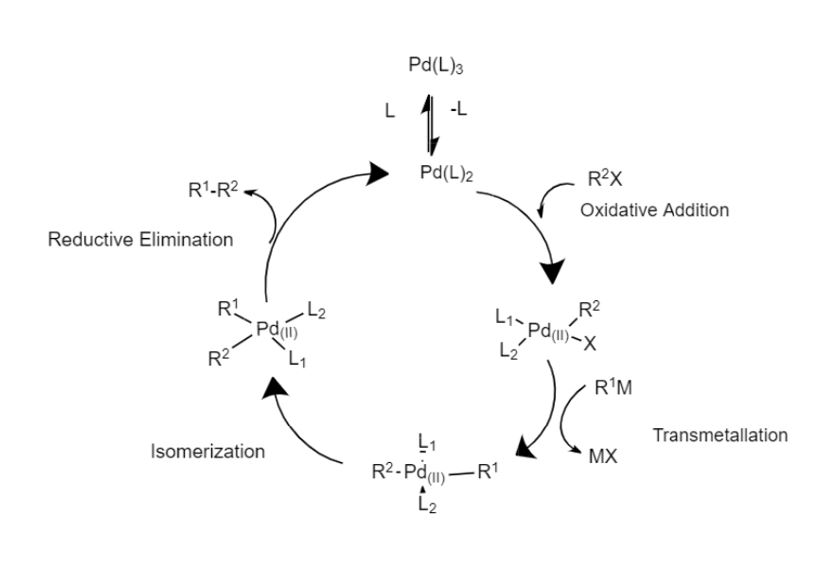
Catalytic cycle

Examples of C-C Cross Coupling Reaction
[edit | edit source]
C=M Complexes
C=M complex is an organometallic complex containing metal-carbon double bonds, in which a σ bond and a π bond present. There are two main carbene complex types: Fischer type(carbene) and Schrock type(alkylidene). Fischer type carbene complex, which was developed in 1964, contains a σ donor on carbon and a π-back donate on metal. Schrock-type carbene complexes, which was developed by Schrock several years later, contains more over sharing electrons and commonly known as alkylidenes. Yves Chauvin, Robert Grubbs, Ricahrd Schrock were awarded the 2005 Nobel prize in chemistry. "for the development of the metathesis method in organic synthesis."[3]
Structure
[edit | edit source]
Fisher-Type Carbene Complexes
[edit | edit source]A carbon on Fisher type is electrophilic because σ donates from the metal to the carbon and has weak back-bonding. Carbon complexes on Fisher have low oxidation state with 18 electron count. For example, Fe(0), Mo(0), Cr(0) (middle to late transition metal) contain good π acceptors ligands in the complex. The stability of Fischer-Type carbene complex can also be enhanced by containing highly electronegative heteroatoms such as O, N, and S. These characteristics of Fischer-Type carbene complex allows to have double bond with Oxygen. The length between these two double bonds in complexes is longer than normal M=C double bond, and shorter than normal M-C single bond. Likewise, the C-X bond distance is shorter than normal C-X bond.
The highly electronegative heteroatoms tend to participate in the π-back bonding with d orbital on the metal, and p orbitals on the carbon. A lone pair is donated from a carbon to an empty d orbital on the metal and another lone pair is donated from π back donate metal to orbital on carbon. An electron pair corporate in σ donation and there is empty π* orbital which takes π back-donation in MO diagram. Bonding is most likely close to CO bond, and good electrons for back donation with good π acceptor. An example of Fischer-Type carbene complexes is the compound with a Cr(0).[4]

![{\displaystyle Cr(CO)_{5}[C(OCH_{3})C_{6}H_{5}]}](https://wikimedia.org/api/rest_v1/media/math/render/svg/9b7e4e9d324bac0368b7eb5a7e4e6c800f7d73fe)
These resonance form will existing on a temperature-dependent proton NMR (detects the cis and trans separately), and on a carbon NMR. however, π bonding system in complexes of this type will highly more existing on X-ray crystallography(shows double bond character).
Schrock-Type Carbene Complexes
[edit | edit source]A carbon on Schrock-Type is nucleophilic, because back-bonding metal is strong and contributes σ donation from the ligand to the metal. Carbon complexes on Schrock have high valence oxidation state with 10-18 electron count. For example, Ti(IV), Ta(V), W(VI) (early transition metal) containing good σ or π donor ligands in the complex. An electron help to form σ bond and π bond in MO diagram. It mostly like compose with H or alkyl, which are directly attached to the carbene. These complexes is composed with two covalent bond interactions. one electron donates to the σ bond from each metal and each carbene. An example of Schrock-Type carbene complexes is the compound with a Ta(V).[5]

These Schrock-Type carbene complexes have M-C-R linkage and make bond angle of 160-170°. Schrock Carbenes can be displayed by proton NMR, carbon NMR, Infrared Spectroscopy, and Raman Spectroscopy. This complex type displays coupling constant values for typical and agostic interaction between the carbene proton and the metal. These techniques are well used to determine bond angles and structures for Schrock-Type carbene complexes.
Synthesis
[edit | edit source]
Fisher Carbene
[edit | edit source]Fisher Carbenes' carbon is an electrophilic. Nucleophilic attack at a carbonyl ligand, and most common method.
Alkyl lithium is attaching on metal carbonyl. Zwitterionic resonance is forming by attaching heteroatom to carbene to stabilize Fischer carbenes. Intermediate of Fisher Carbenes is treated as electrophilic to give the Fisher carbene. C-X bond rotation is restricted in syn and anti isomers for alkyl derivatives at low temperature proton NMR because zwitterion resonance forms in Fischer carbenes. These can be observed by X-ray crystallography.

Schrock Carbenes
[edit | edit source]Schrock Carbenes' carbon is a nucleophilic. There is α-abstraction in the Schrock carbenes synthesis and induced by steric bulk. Schrock carbene is the main key for both reagents and catalysts. The most famous examples for Schrock Carbenes synthesis are Patasis' Reagent, Tebbe's Reagent, and Grubb's Catalyst. Schrock Carbenes synthesis is used to widespread reactivity such as intermediate of the preparation of organometallic. The most famous of Schrock Carbenes reactivity is Olefin Metathesis
Reactivity
[edit | edit source]Olefin Metathesis
[edit | edit source]Olefin metathesis is the main application for carbene. Olefin metathesis reaction utilizes two alkenes to make cyclobutanes and reform the two new types of double bond. A reaction of olefin metathesis works rapidly. d orbitals on the metal alkylidene is present, and it breaks cyclobutanes symmetry and reacts very quickly. Normally, the products of olefin metathesis are statistical, unless the reaction can be driven is some way or the tow alkenes have different reactivities.[6] Titanium, Tungsten, Molybdenum, and Ruthenium are the popular metal for olefin metathesis.
There are five different kinds of reactions process of Olefin Metathesis:
- Cross metathesis CM
- ring-closing metathesis RCM
- ring-opening metathesis ROM
- ring-opening metathesis polymerization ROMP
- acyclic diene metathesis polymerization ADMET
References
[edit | edit source]- ↑ Miessler, G.(2014)Inorganic Chemistry- 5th Edition. Upper Saddle River, NJ: Pearson Education, Inc.pp.541-548
- ↑ https://www.chem.tamu.edu/rgroup/marcetta/chem462/lectures/Eshon-Vangal-Cross%20Coupling%20Reactions.pdf
- ↑ "2005 nobel prize in chemistry".
- ↑ Misseler, Gary L (2012). Inorganic Chemistry. Boston: Pearson. p. 515.
- ↑ Gary L., Miessler (2012). Inorganic Chemistry. Boston: Pearson. p. 516.
- ↑ "Chem &Eng News 2002, Dec 23, 34-38". http://nobelprize.org/nobel_prizes/chemistry/laureates/2005/animation.html.
Olefin Metathesis
Olefin Metathesis is an organic chemical reaction that uses a metal catalyst for the transfer of substituents between olefins, or alkenes by a 4-membered ring intermediate, also known as a Chauvin Mechanism. This efficient method does not only have a high yield, but it produces less byproducts and hazardous waste compared to other organic reactions. Yves Chauvin, Robert H. Grubbs and Richard R. Schrock won The Nobel Prize in Chemistry of 2005 for their contributions to olefin metathesis.
Historical Overview
[edit | edit source]Herbert S. Eleuterio, an industrial chemist in the 1950s, found a propylene-ethylene copolymer from a propylene feed on a Mo-Al catalyst as a result of his experiment. He repeated the experiment with a cyclopentene and noticed that “the polymer looked like somebody took a pair of scissors, opened up cyclopentene, and neatly sewed it up again.” Other chemists were also getting similar results of the cleavage and reformation of the olefin double bonds. To his understanding, Grubbs suggested that the rearrangement of substituents occurred through a metallacyclopentane intermediate. Chauvin proposed that olefin metathesis is initiated by a metal carbene. Many scientists agreed with Chauvin that metal carbenes played a major role in the process of olefin metathesis and from there, it was further studied to understand the full mechanism.
Mechanism
[edit | edit source]The rearrangement of substituents on two olefins occurs through the formation of a 4-membered ring intermediate as in the following figure.
The initial alkene with substituent R1 forms an intermediate with an olefin metal carbene, allowing the metal element to be attached to the initial alkene. The product then reacts with a second alkene with substituent R2, forming another 4-membered ring intermediate and yields a final combined olefin with both R1 and R2 substituents while producing back the initial metal carbene. This type of 4-membered ring formation is called a [2+2] cycloaddition. A 4-membered ring is not the most stable and is known to cause strain on the molecule. As a result, the formation has a very high activation energy. Interaction with the metal lowers the activation energy of the ring formation, allowing the process to occur at moderate temperatures.
Catalyst
[edit | edit source]Olefin Metathesis requires the application of a metal catalysts. The most common catalysts used are Grubbs catalyst and Schrock catalyst.
Grubbs catalyst is a commercially available catalyst and is easy to handle as it is pretty stable against water, oxygen, and other small impurities. Although it has its advantages like high functional group tolerance, there is a drawback in that it has a lower reactivity compared to other catalysts like the Mo Imido Alkylidene Catalyst.

Upon interaction with an olefin, a 4-membered ring is formed cis to the carbene and trans to the Cl atoms.

Like the Grubbs catalyst, the Schrock catalyst is also commercially available. It has a higher reactivity than the Grubbs catalyst and is tolerant of multiple functional groups, but has many disadvantages such as needing to be handled under an inert atmosphere using dry solvents and substrates as well as being intolerant to protons on heteroatoms.
Basic Types of Metathesis
[edit | edit source]- Ring Opening Metathesis Polymerization (ROMP)
- Ring Closing Metathesis (RCM)
- Cross Metathesis (CM)
- Acyclic Diene Metathesis Polymerization (ADMET)
Applications
[edit | edit source]Olefin metathesis opened up new industrial pathways for petrochemicals, polymers, and so much more. In the petrochemical field, olefin metathesis is used for the Olefins Conversion Technology (OCT) Process and the Shell Higher Olefins Process (SHOP). ROMP has opened up an opportunity to generate useful polymers with special properties in many industrial methods. For future oleochemical advancements, metathesis of natural fats has opened a door of possibilities. Currently, the most important applications are used to make propene, detergent-range olefins, and polymers.
References
[edit | edit source]- Jen, W. "Olefin Metathesis in Organic Synthesis".
{{cite journal}}: Cite journal requires|journal=(help) - Mol, J.C. "Industrial Applications of Olefin Metathesis". 213 (1): 39–45. doi:10.1016/j.molcata.2003.10.049.
{{cite journal}}: Cite journal requires|journal=(help) - Rouhi, A.M. "Olefin Metathesis: The Early Days". 80 (51): 34–38.
{{cite journal}}: Cite journal requires|journal=(help)