Linear Algebra/Systems of linear equations

Our study of linear algebra will begin with examining systems of linear equations. Such linear equations appear frequently in applied mathematics in modelling certain phenomena. For example in linear programming, profit is usually maximized subject to certain constraints related to labour, time availability etc. These constraints can be put in the form of a linear system of equations.

While we have already studied the contents of this chapter (see Algebra/Systems of Equations) it is a good idea to quickly re read this page to freshen up the definitions.

Linear systems

Graph sample of linear equations

A linear equation is an equation in which each term is either a constant or the product of a constant times the first power of a variable. Such an equation is equivalent to equating a first-degree polynomial to zero. Some examples of linear equations are as follows:

• $x+3y=-4\$
• $7x_{1}=15+x_{2}\$
• $z{\sqrt {2}}+e=\pi \$

The term linear comes from basic algebra and plane geometry where the standard form of algebraic representation of a line that is on the real plane is $ax+by=c$ where a, b, c are real constants and x, y are real variables. Review of the above examples will find each equation fits the general form.

The following are not linear equations:

• $xy+7=2\$
• ${\sqrt {x_{1}}}+x_{2}=11$
• $x^{3}=6-12z\$

For an equation to be linear, it does not necessarily have to be in standard form (all terms with variables on the left-hand side). The constants in linear equations need not be integral (or even rational).

Linear equations are classified by the number of variables they involve. The classification is straightforward -- an equation with n variables is called a linear equation in n variables. If n is 2 the linear equation is geometrically a straight line, and if n is 3 it is a plane. The geometrical shape for a general n is sometimes referred to as an affine hyperplane. We'll however be simply using the word n-plane for all n.

For clarity and simplicity, a linear equation in n variables is written in the form $a_{1}x_{1}+a_{2}x_{2}+a_{3}x_{3}+...+a_{n}x_{n}=b\$, where $a_{1},a_{2},...,a_{n}\$ are constants (called the coefficients), and $b\$ is the constant term.

A linear system in three variables determines a collection of planes.

A linear system (or system of linear equations) is a collection of linear equations involving the same set of variables. For example,

${\begin{alignedat}{7}3x&&\;+\;&&2y&&\;-\;&&z&&\;=\;&&1&\\2x&&\;-\;&&2y&&\;+\;&&4z&&\;=\;&&-2&\\-x&&\;+\;&&{\tfrac {1}{2}}y&&\;-\;&&z&&\;=\;&&0&\end{alignedat}}$

is a system of three equations in the three variables $x,y,z\,\!$.

A general system of m linear equations with n unknowns (or variables) can be written as

${\begin{alignedat}{7}a_{11}x_{1}&&\;+\;&&a_{12}x_{2}&&\;+\cdots +\;&&a_{1n}x_{n}&&\;=\;&&&b_{1}\\a_{21}x_{1}&&\;+\;&&a_{22}x_{2}&&\;+\cdots +\;&&a_{2n}x_{n}&&\;=\;&&&b_{2}\\\vdots \;\;\;&&&&\vdots \;\;\;&&&&\vdots \;\;\;&&&&&\;\vdots \\a_{m1}x_{1}&&\;+\;&&a_{m2}x_{2}&&\;+\cdots +\;&&a_{mn}x_{n}&&\;=\;&&&b_{m}\\\end{alignedat}}$

Here $x_{1},\ x_{2},...,x_{n}$ are the unknowns, $a_{11},\ a_{12},...,\ a_{mn}$ are the coefficients of the system, and $b_{1},\ b_{2},...,b_{m}$ are the constant terms.

Solutions of linear systems

A solution of a linear equation is any n-tuple of values $(s_{1},s_{2},....,s_{n})\$which satisfies the linear equation. For example, $(-1,-1)\$ is a solution of the linear equation $x+3y=-4\$ since $-1+(3\times -1)=-1+(-3)=-4$, but $(1,5)\$ is not.

Similarly, a solution to a linear system is any n-tuple of values $(s_{1},s_{2},....,s_{n})\$which simultaneously satisfies all the linear equations given in the system.

For example,

${\begin{alignedat}{7}3x&&\;+\;&&2y&&\;-\;&&z&&\;=\;&&1&\\2x&&\;-\;&&2y&&\;+\;&&4z&&\;=\;&&-2&\\-x&&\;+\;&&{\tfrac {1}{2}}y&&\;-\;&&z&&\;=\;&&0&\end{alignedat}}$

has as its solution $(1,-2,-2)\$. This can also be written as:

${\begin{alignedat}{2}x&=&1\\y&=&-2\\z&=&-2\end{alignedat}}$

We also refer to the collection of all possible solutions as the solution set.

In general, for any linear system of equations there are three possibilities regarding solutions:

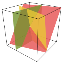
A unique solution: In this case only one specific solution set exists. Geometrically this implies the n-planes specified by each equation of the linear system all intersect at a unique point in the space that is specified by the variables of the system.

No solution: The equations are termed inconsistent and specify n-planes in space which do not intersect or overlap. It is not possible to specify a solution set that satisfies all equations of the system.

An infinite range of solutions: The equations specify n-planes whose intersection is an m-plane where $m\leq n$. This being the case, it is possible to show that an infinite set of solutions within a specific range exists that satisfy the set of linear equations.

The following pictures illustrate these cases:

A unique solution	No solution	An infinite range of solutions

Why are there only these three cases and no others? Although a justification shall be provided in the next chapter, it is a good exercise for you to figure it out now.

A linear system is said to be inconsistent if it has no solution. If there exists at least one solution, then the system is said to be consistent.

Methods of solving linear systems

We know that linear equations in 2 or 3 variables can be solved using techniques such as the addition and the substitution method. However these techniques are not appropriate for dealing with large systems where there are a large number of variables. These techniques are therefore generalized and a systematic procedure called Gaussian elimination is usually used in actual practice. We will study this in a later chapter. A variant of this technique known as the Gauss Jordan method is also used.

Many times we are required to solve many linear systems where the only difference in them are the constant terms. The coefficients of the variables all remain the same. A technique called LU decomposition is used in this case. A variant called Cholesky factorization is also used when possible. We will study these techniques in later chapters.

Exercises

This chapter is meant as a review. There are no exercises. find the solution set to the following systems 1.x1+2x2+3x3-4x4+5x5=25