The mean and variance of some distributions (which have simple formulas for mean and variance) will be discussed in the properties of distribution chapter.
Consider independent Bernoulli trials with the same success probability .
We would like to calculate to probability .
Let be the event , as in the previous section.
Let's consider a particular sequence of outcomes such that there are successes in trials:
Its probability is
[2]
Since the probability of other sequences with some of successes occurring in other trials is the same,
and there are distinct possible sequences[3],
This is the pmf of a random variable following the binomial distribution.
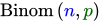
A random variable follows the binomial distribution with independent Bernoulli trials and success probability , denoted by , if its pmf is
Cdf's of and .
Remark.
The "" in the pmf emphasizes that the values of parameters of the distribution (which are quantities that describes the distribution) are and . We can similar notations to pdf.
There are some alternative notations for emphasizing the parameter values. For example, when the parameter value is , then the pdf/pmf can be denoted by
Of course, it is not necessary to adding these to the pdf/pmf, but it makes the parameter values involved explicit and clear.
The pmf involves a binomial coefficient, and hence the name 'binomial distribution'.
General remark for each distribution:
We may also just write down the notation for the distribution to denote the distribution itself, e.g. stands for the binomial distribution.
We sometimes say pmf, pdf, or support of a distribution, to mean pmf, pdf or support (respectively) of a random variable following that distribution, for simplicity (it also applies for other properties of distribution (discussed in a later chapter), e.g. mean, variance, etc.).
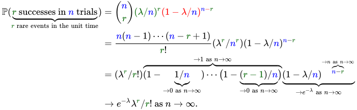
The Poisson distribution can be viewed as the 'limit case' for the binomial distribution.
Consider independent Bernoulli trials with success probability . By the binomial distribution,
After that, consider an unit time interval, with (positive) occurrence rate of a rare event (i.e. the mean of number of occurrence of the rare event is ). We can divide the unit time interval to time subintervals of time length each.
If is large and is relatively small, such that the probability for
occurrence of two or more rare events at a single time interval is negligible, then the probability for occurrence of exactly one rare event
for each time subinterval is by definition of mean.
Then, we can view the unit time interval as a sequence of Bernoulli trials [4] with success probability .
After that, we can use to model the number of occurrences of rare event. To be more precise,
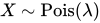
This is the pmf of a random variable following the Poisson distribution,
and this result is known as the Poisson limit theorem (or law of rare events). We will introduce it formally after introducing the definition of Poisson distribution.
Consider a sequence of independent Bernoulli trials with success probability .
We would like to calculate the probability .
By considering this sequence of outcomes:
we can calculate that
[5]
This is the pmf of a random variable following the geometric distribution.
A random variable follows the geometric distribution with success probability, denoted by , if its pmf is
Cdf's of and .
Remark.
The sequence of the probabilities starting from , with input value increased one by one (i.e. ) is a geometric sequence, and hence the name 'geometric distribution'.
For an alternative definition, the pmf is instead , which is the proability , with support .
Proposition.
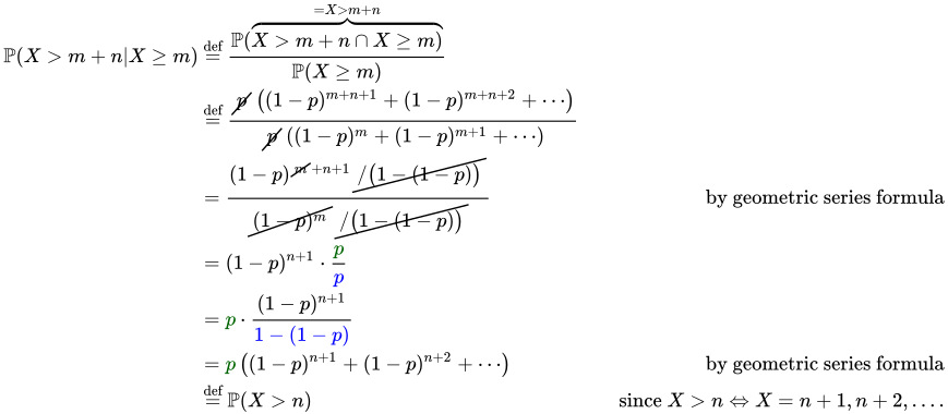
(Memorylessness of geometric distribution)
If , then
for each nonnegative integer and .
Proof.
In particular, since .
Remark.
can be interpreted as 'there are more than failures before the first success';
can be interpreted as ' failures have occured, so there are more than or equal to failures before the first success'.
It implies that the condition does not affect the distribution of the remaining number of failures before the first success (it still follows geometric distribution with the same success probability).
So, we can assume the trials start afresh after an arbitrary trial for which failure occurs.
E.g., if failure occurs in first trial, then the distribution of the remaining number of failures before the first success is not affected.
Also, if success occurs in first trial, then the condition becomes , instead of , so the above formula cannot be applied in this situation.
Consider a sequence of independent Bernoulli trials with success probability .
We would like to calculate the probability .
By considering this sequence of outcomes:
we can calculate that
Since the probability of other sequences with
some of failures occuring in other trials
(and some of successes (excluding the th success,
which must occur in the last trial) occuring in other trials), is the same, and there are
(or ,
which is the same numerically) distinct possible sequences
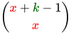
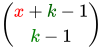
[6],
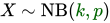
This is the pmf of a random variable following the negative binomial distribution.
Consider a sample of size are drawn without replacement
from a population size , containing objects of type 1 and of another type.
Then, the probability
[7].
: unordered selection of objects of type 1 from (distinguishable) objects of type 1 without replacement;
: unordered selection of objects of another type from (distinguishable) objects of another type without replacement;
: unordered selection of objects from (distinguishable) objects without replacement.
This is the pmf of a random variable following the hypergeometric distribution.
A random variable follows the hypergeometric distribution with objects drawn from a collection of objects of type 1 and of another type, denoted by , if its pmf is
Cdf's of and .
Remark.
The pmf is sort of similar to hypergeometric series [8], and hence the name 'hypergeometric distribution'.
This type of distribution is a generalization of all discrete distribution with finite support, e.g. Bernoulli distribution and hypergeometric distribution.
Another special case of this type of distribution is discrete uniform distribution, which is similar to the continuous uniform distribution (will be discussed later).
Definition.
(Finite discrete distribution)
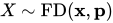
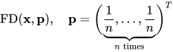
A random variable follows the finite discrete distribution with vector and probability vector ,
denoted by if its pmf is
Remark.
For mean and variance, we can calculate them by definition directly. There are no special formulas for finite discrete distribution.
Definition.
(Discrete uniform distribution)
The discrete uniform distribution, denoted by , is .
Remark.
Its pmf is
Example.
Suppose a r.v. .
Then,
Illustration of the pmf:
The continuous uniform distribution is a model for 'no preference',
i.e. all intervals of the same length on its support are equally likely[9] (it can be seen from the pdf corresponding to continuous uniform distribution).
There is also discrete uniform distribution, but it is less important than continuous uniform distribution.
So, from now on, simply 'uniform distribution' refers to the continuous one, instead of the discrete one.
Definition.
(Uniform distribution)
Pdf's of .
A random variable follows the uniform distribution, denoted by , if its pdf is
Remark.
The support of can also be alternatively or , without affecting the probabilities of events involved, since the probability calculated, using pdf at a single point, is zero anyways.
The distribution is the standard uniform distribution.
The exponential distribution with rate parameter is often used to describe the interarrival time of rare events with rate .
Comparing this with the Poisson distribution, the exponential distribution describes the interarrival time of rare events,
while Poisson distribution describes the number of occurrences of rare events within a fixed time interval.
By definition of rate, when the rate, then interarrival time (i.e. frequency of the rare event ).
So, we would like the pdf to be more skewed to left when (i.e. the pdf has higher value for small when ), so that areas under the pdf for intervals involving small value of when .
Also, since with a fixed rate , the interarrival time should be less likely of higher value. So, intuitively, we would also like the pdf to be a strictly decreasing function, so that the probability involved (area under the pdf for some interval) when .
As we can see, the pdf of exponential distribution satisfies both of these properties.
Definition.
(Exponential distribution)
Pdf's of and .
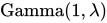
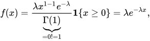
A random variable follows the exponential distribution with positive rate parameter , denoted by , if its pdf is
Proposition.
(Cdf of exponential distribution)
Cdf's of and .
The cdf of is
Proof.
Suppose . The cdf of is
Proposition.
(Memorylessness of exponential distribution)
If , then
for each nonnegative number and .
Proof.
Remark.
can be interpreted as 'the rare event will not occur within next units of time';
can be interpreted as 'the rare event has not occurred for past units of time'.
It implies that the condition does not affect the distribution of the remaining waiting time for the rare event (it still follows exponential distribution with the same parameter).
So, we can assume the arrival process of the event starts afresh at arbitrary time point of observation.
The Cauchy distribution is a heavy-tailed distribution [10].
As a result, it is a 'pathological' distribution, in the sense that it has some counter-intuitive properties, e.g. undefined mean and variance, despite its mean and variance seems to be defined when we look at its graph directly.
Definition.
(Cauchy distribution)
Pdf and cdf of .
A random variable follows the Cauchy distribution with location parameter , denoted by , if its pdf is
Remark.
This definition is referring to a special case of Cauchy distribution. To be more precise, there is also the scale parameter in the complete definition of Cauchy distribution, and it is set to be one in the pdf here.
The normal or Gaussian distribution is a thing of beauty, appearing in many places in nature. This is probably because sample means or sample sums often follow normal distributions approximately
by central limit theorem.
As a result, the normal distribution is important in statistics.
Definition.
(Normal distribution)
Pdf's of and .
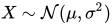
A random variable follows the normal distribution with mean and variance,
denoted by , if its pdf is
Cdf's of and .
Remark.
The distribution is the standard normal distribution.
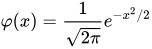
For , its pdf is often denoted by , and its cdf is often denoted by .
pdf of is .
It follows that the pdf of is .
It will be proved that is actually the mean, and is actually the variance.
The pdf is symmetric about , since .
Proposition.
(Distributions for linear transformation of normally distributed random variables)
If , and
and are constants,
.
Proof.
Assume [11].
Let and be cdf of and respectively.
Since
by differentiation,
which is the pdf of .
Remark.
A special case is when and , since
;
.
This shows that we can transform each normally distributed r.v. to the r.v. following standard normal distribution.
This can ease the calculation for the probability relating the normally distributed r.v., since we have the standard normal table, in which values of at different are given.
For some types of standard normal table, only the values of at different nonnegative are given.
Then, we can calculate its values at different negative using
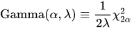
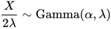
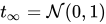
The -distribution is sort of a generalized Student's -distribution, in the sense that it has one more changeable parameter for another degrees of freedom.
Definition.
(-distribution)
The -distribution with and degrees of freedom, denoted by ,
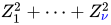
is the distribution of in which and .
Pdf's of and .Cdf's of and .
Remark.
.
A random variable following the -distribution with and degrees of freedom is denoted by .
It can be proved that the pdf of is
If you are interested in knowing how chi-squared distribution, Student's -distribution, and -distribution are useful in statistics,
then you may briefly look at, for instance, Statistics/Interval Estimation (applications in confidence interval construction) and Statistics/Hypothesis Testing (applications in hypothesis testing).
Multinomial distribution is generalized binomial distribution,
in the sense that each trial has more than two outcomes.
Suppose objects are to be allocated to cells independently,
for which each object is allocated to one and only one cell, with probability to be allocated to the th cell () [12].
Let be the number of objects allocated to cell .
We would like to calculate the probability , i.e.
the probability that th cell has objects.
We can regard each allocation as an independent trial with outcomes (since it can be allocated to one and only one of cells).
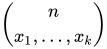
We can recognize that the allocation of objects is partition of objects into groups. There are hence ways of allocation.
So,
In particular, the probability of allocating objects to th cell is by independence, and so that of a particular case of allocation of objects to cells is
by independence.
Definition.
(Multinomial distribution)
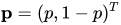
A random vector follows the multinomial distribution with trials and probability vector ,
denoted by , if its joint pmf is
Remark.
if .
In this case, if , is the number of successes for the binomial distribution (and is the number of failures).
Also, . It can be seen by regarding allocating the object into th cell as 'success' for each allocation of single object [13]. Then, the success probability is .
Multivariate normal distribution is, as suggested by its name, a multivariate (and also generalized) version of the normal distribution (univariate).
Definition.
(Multivariate normal distribution)
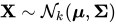
A random vector follows the -dimensional normal distribution
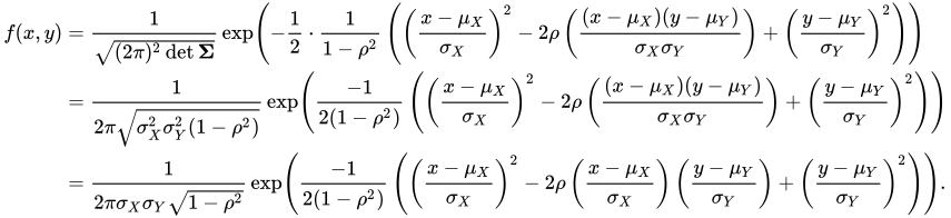
with mean vector and covariance matrix, denoted by [14] if its joint pdf is
in which
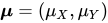
is the mean vector,
and is the covariance matrix (with size ).
Remark.
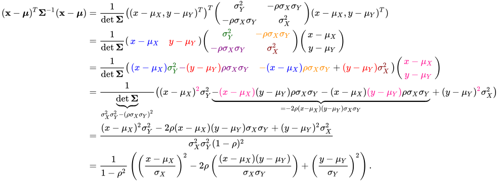
The distribution for case is more usually used, and that is called the bivariate normal distribution.
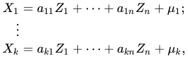
An alternative and equivalent definition is that if
for some constants , and are i.i.d. standard normal random variables.
Using the above result, the marginal distribution followed by is , as one will expect.
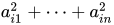
By proposition about the sum of independent normal random variables and distribution of linear transformation of normal random variables (see Probability/Transformation of Random Variables chapter), the mean is , and the variance is (this equals by definition).
↑This is because there is unordered selection of (distinguishable and ordered) trials for 'success' without replacement from trials (then the remaining position is for 'failure').
↑Occurrence of the rare event is viewed as 'success' and non-occurrence of the rare event is viewed as 'failure'.
↑Unlike the outcomes for the binomial distribution, there is only one possible sequence for each .
↑There is unordered selection of trials for 'failures' (or
trials for 'successes') from trials without replacement
↑The restriction on is imposed so that the binomial coefficients are defined, i.e. the expression 'makes sense'. In practice, we rarely use this condition directly. Instead, we usually directly determine whether a specific value of 'makes sense'.
↑The probability is 'distributed uniformly over an interval'.
↑A random variable following the Cauchy distribution has a relatively high probability to take extreme values, compared with other light-tailed distributions (e.g. the normal distribution). Graphically, the 'tails' (i.e. left end and right end) of the pdf.
↑The case for holds similarly (The inequality sign is in opposite direction, and eventually we will have two negative signs cancelling each other). Also when , the r.v. becomes a non-random constant, and so we are not interested in this case.































































































![{\displaystyle {\color {dodgerblue}{\mathcal {U}}[a,b]}}](https://wikimedia.org/api/rest_v1/media/math/render/svg/3e43064f6f5b6b3782a88f679aff01f560a756a5)
![{\displaystyle X\sim {\mathcal {U}}[a,b]}](https://wikimedia.org/api/rest_v1/media/math/render/svg/4ef8f0bf7ccaa764ee9bf60944dec51559aa8a09)
![{\displaystyle f(x)=1/(b-a),\quad x\in \operatorname {supp} (X)=[a,b],{\text{ and }}a\leq b.}](https://wikimedia.org/api/rest_v1/media/math/render/svg/1b9538bcba07e181297d1ea8bed39125abf37e33)
![{\displaystyle {\mathcal {U}}[a,b]}](https://wikimedia.org/api/rest_v1/media/math/render/svg/140992400aff9597adf2989ac9a7c4540902ebe5)
![{\displaystyle [a,b),(a,b]}](https://wikimedia.org/api/rest_v1/media/math/render/svg/c831c660bc5d57d59b3c2fb8e01b633bf726ba32)

![{\displaystyle {\mathcal {U}}[0,1]}](https://wikimedia.org/api/rest_v1/media/math/render/svg/b1aec3afe927b9042f55a8c5ea4cbd1d9d97de55)


![{\displaystyle F(x)=\int _{-\infty }^{x}{\frac {\mathbf {1} \{a\leq x\leq b\}}{b-a}}\,dy={\frac {1}{b-a}}\int _{a}^{x}\mathbf {1} \{a\leq x\leq b\}\,dy={\begin{cases}0/(b-a),&x<a;\\[][y]_{a}^{x}/(b-a),&a\leq x\leq b;\\[][y]_{a}^{b}/(b-a),&x>b.\end{cases}}}](https://wikimedia.org/api/rest_v1/media/math/render/svg/2f1c057e9f6b1f0ddf5f74f1a8dcde00a4b52790)









![{\displaystyle {\begin{aligned}F(x)&=\int _{-\infty }^{x}\lambda e^{-\lambda y}\mathbf {1} \{y\geq 0\}\,dy\\&={\begin{cases}\int _{0}^{x}\lambda e^{-\lambda y}\,dy,&x\geq 0;\\0,&x<0\\\end{cases}}&\left({\text{When }}x<0,x\notin \operatorname {supp} (X),{\text{ so }}F(x)=\mathbb {P} (X\leq x)=0\right)\\&=\mathbf {1} \{x\geq 0\}\lambda \int _{0}^{x}e^{-\lambda y}\,dy\\&=\mathbf {1} \{x\geq 0\}{\frac {\lambda }{-\lambda }}[e^{-\lambda }y]_{0}^{x}\\&=-\mathbf {1} \{x\geq 0\}(e^{-\lambda x}-1)\\&=(1-e^{-\lambda x})\mathbf {1} \{x\geq 0\}.\\\end{aligned}}}](https://wikimedia.org/api/rest_v1/media/math/render/svg/81bc9a6589d70ff54a7647210bf48053e9e59e92)
















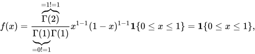
![{\displaystyle f(x)={\frac {\Gamma (\alpha +\beta )}{\Gamma (\alpha )\Gamma (\beta )}}x^{\alpha -1}(1-x)^{\beta -1},\quad x\in \operatorname {supp} (X)=[0,1].}](https://wikimedia.org/api/rest_v1/media/math/render/svg/7299f58655ef8cd2a8476dcda38fd376229ceba2)

![{\displaystyle \operatorname {Beta} (1,1)\equiv {\mathcal {U}}[0,1]}](https://wikimedia.org/api/rest_v1/media/math/render/svg/ed813cf144d2362a448c73758ddbdda1dfe15fd1)
































![{\displaystyle {\begin{aligned}&&\phi (-y)&=\phi (y)\\&\Leftrightarrow &\int _{-\infty }^{x}\phi (-y)\,dy&=\int _{-\infty }^{x}\phi (y)\,dy\\&\Leftrightarrow &-\int _{\infty }^{-x}\phi (u)\,du&=\Phi (x)&{\text{let }}u=-y\Rightarrow dy=-dy.\\&\Leftrightarrow &[\Phi (u)]_{-x}^{\infty }&=\Phi (x)\\&\Leftrightarrow &\underbrace {\Phi (\infty )} _{=\mathbb {P} (\Omega )=1}-\Phi (-x)&=\Phi (x).\end{aligned}}}](https://wikimedia.org/api/rest_v1/media/math/render/svg/2cbcad71d39070a50f0c1c54a6378e488452564d)










































![{\displaystyle {\boldsymbol {\mu }}=(\mu _{1},\dotsc ,\mu _{k})^{T}=(\mathbb {E} [X_{1}],\dotsc ,\mathbb {E} [X_{k}])^{T}}](https://wikimedia.org/api/rest_v1/media/math/render/svg/4f6f4faa98c1603023d57740ff2ae0fb06ba5406)