Practical Guide to Gaussian Processes
Preface
[edit | edit source]This book gives an introduction to Gaussian processes and shows their various, but not complete, applications. The introduction is aimed for users who want to apply the technique to solve practical engineering problems. With application examples, it shows how Gaussian processes can be used for machine learning to infer from known to unknown situations. The book serves as a reference for common analytical representations of Gaussian processes and for mathematical operations and methods in specific use cases.
Introduction
[edit | edit source]A Gaussian process is a stochastic process with the property that every finite subset of its values is multivariate normally distributed (or Gaussian distributed). A stochastic process is a function whose values are random variables and which follow a given probability distribution. This allows to model functions with probabilities whose values cannot be completely determined due to a lack of information. A Gaussian process is constructed from functions of mean values, variances and covariances and thus describes the function values as a continuum of correlated random variables in the form of an infinite-dimensional normal distribution. The distribution of a Gaussian process can be imagined as a probability distribution of functions. A sample of it yields a random function with certain preferred properties of its curve shape.
Applications
[edit | edit source]Gaussian processes are used for mathematical modeling of the behavior of non-deterministic systems on the basis of stochastic quantities or observations. Gaussian processes are suitable for signal analysis and synthesis, form a powerful tool for the interpolation, extrapolation, or smoothing of arbitrarily dimensional discrete measurement points (Gaussian process regression or kriging), and find application in classification problems. Gaussian processes, which are related to kernel methods,[1] can be used as a supervised machine learning technique for abstract modeling based on training examples. This Bayesian approach to machine learning has the advantage that it often does not require iterative training as neural networks do. Instead, Gaussian processes can be derived very efficiently with linear algebra from statistical quantities of the examples and are mathematically clearly interpretable and well controllable. Moreover, for interpolations and predictions, an associated confidence interval is computed for each individual output value, which accurately estimates its own prediction error, while correctly accounting for error propagation when the variance of the input values is known.
Mathematical Description
[edit | edit source]Definition
[edit | edit source]A Gaussian process is a special type of stochastic process on any index set , if its finite-dimensional distributions are multivariate normal distributions (also Gaussian distributions) for all . That is, the multivariate distribution of is given by an n-dimensional normal distribution.


Term: Even the term Gaussian process may indicate temporal or sequential processes, this restriction does not exist. In a generalized sense, process can be understood as a continuum.
Notation
[edit | edit source]In analogy to the one- and multidimensional Gaussian distribution, a Gaussian process is completely and uniquely determined by its first two moments. In the multidimensional Gaussian distribution, these are the expected value vector or mean vector and the covariance matrix . For the description of Gaussian process, these are replaced by an expected value function or mean function


and a covariance function
- .
![{\displaystyle k(t,t'):=\operatorname {Cov} (X_{t},X_{t'}):=\mathbb {E} \left[(X_{t}-m(t))\cdot (X_{t'}-m(t'))\right],\quad t,t'\in T}](https://wikimedia.org/api/rest_v1/media/math/render/svg/4aa08ac5d45b1abae6327583cdf7187d367347ff)
These functions can be understood in the simplest one-dimensional case as a vector with continuous rows and as a matrix with continuous rows and columns. The following table compares one-dimensional and multidimensional Gaussian distributions with Gaussian processes. The tilde symbol can be read as "is distributed as".

| Distribution type | Notation | Variables | Probability density function |
|---|---|---|---|
| Univerate normal distribution | |||
| Multivariate normal distribution | |||
| Gaussian process distribution | (no analytical representation) |


The probability density function of a Gaussian process cannot be represented analytically because there is no corresponding notation for operations with continuous matrices. This gives the impression that one cannot perform computations with Gaussian processes in the same way as with finite-dimensional normal distributions. However, the essential property of the Gaussian process is not the infinity of the dimensions, but rather the assignment of the dimensions to the coordinates of a function. In practical applications, one always has to deal with a finite number of interpolation points and can therefore perform all calculations as in the finite-dimensional case. The limit to infinitely many dimensions is only needed in an intermediate step, namely if values are to be read out at new interpolated grid points. In this intermediate step, the Gaussian process, i.e. the mean function and covariance function, is represented or approximated by suitable analytical expressions. In this case the assignment to the grid points is done via the parameterized coordinates in the analytical expression. In the finite-dimensional case with discrete grid points the associated coordinates are assigned to the dimensions by their indices.


Example of a Gaussian process
[edit | edit source]As a simple real world example, consider a Gaussian process

with a scalar variable (time), given by the mean function

and covariance function

This Gaussian process describes an endless temporal electrical signal with Gaussian white noise with a standard deviation of one volt centered around a mean voltage of 5 volts.
Definitions of special properties
[edit | edit source]A Gaussian process is called centered if its expected value or mean is constantly 0, that is, if for all .


A covariance function is called stationary when it is translation invariant, that is, it can be described by a relative function .[2]


A Gaussian process is called stationary (or translation invariant) if its covariance function is stationary and its mean is constant.[3]
A covariance function is called radial when the function is radial symmetric with a one-dimensional parameter using the Euclidean norm . It is used to describe systems with isotropic model properties.


List of Common Gaussian Processes and Covariance Functions
[edit | edit source]- Constant: and


- Corresponds to a constant value from a Gaussian distribution with standard deviation .
- Offset: and


- Corresponds to a constant value given by .

- Gaussian White noise:

- (: standard deviation, : Kronecker delta)

- Rational quadratic:
- Gamma-exponential:
- Ornstein-Uhlenbeck:[4]


- Corresponds to a simple Gauss-Markov process and describes continuous, non-differentiable functions, as well as white noise after passing through an RC low-pass filter.
- Squared exponential:

- Describes infinitely smooth differentiable functions.
- Matérn: [5]
- A highly versatile Gaussian process used to describe most typical measurement curves. The functions of the Gaussian process are times continuously differentiable if . Covariance functions with , , , etc. correspond to white noise that has passed through 1, 2, or 3 RC low-pass filters or has been convolved with the function . Common special cases include:
- corresponds to the Ornstein-Uhlenbeck covariance function, and corresponds to the squared exponential function.


- Periodic:

- Functions from this Gaussian process are both periodic with period and smooth (squared exponential). If the square around the sine is replaced by the absolute value, non-smooth periodic functions result.
- Polynomial:

- Grows rapidly outward and is usually a poor choice for regression problems, but can be useful in high-dimensional classification problems. It is positive semidefinite and does not necessarily generate invertible covariance matrices.[6]
- Brownian bridge: and
- Wiener process: and


- Corresponds to the Brownian motion or integral over Gaussian white noise.
- Itō process: If and , are two integrable real-valued functions and is a Wiener process, then the Ito process


- is a Gaussian process with and .


Remarks:
- is the distance for stationary and radial covariance functions .
- is the characteristic length scale of the covariance function where the correlation has decayed to about .
- Most stationary covariance functions are normalized to and are therefore equivalent to correlation functions. For use as covariance functions, they are multiplied by a variance , which assigns the variables a scaling and/or physical unit.
- Covariance functions cannot be arbitrary functions or , as it must be ensured that they are positive definite.[7] Positive semidefinite functions are also valid covariance functions, but it should be noted that these do not necessarily result in invertible covariance matrices and are therefore usually combined with a positive definite function.


Mathematical operations with Gaussian processes
[edit | edit source]Gaussian processes (or normal distributions) can be used to perform various stochastic operations that allow different functions with normally distributed errors to be joined or extracted from each other. If there are cross-correlations between the functions, it is assumed that they follow a joint normal distribution. In signal processing, for example, the operations are used to handle temporal signals and their measurement uncertainties. The distributions of these functions are described in the following operations in vector and matrix notation for finitely many interpolation points , which analogously applies to arbitrary mean functions and covariance functions . The normally distributed vectors (, etc.) are described as functions accordingly.


Linear transformation
[edit | edit source]Addition: uncorrelated functions
[edit | edit source]If the sum of two independent (and especially uncorrelated) functions is built, then their mean functions and their covariance functions add up:
- .

The associated probability density functions thereby undergo a convolution.
Addition: correlated functions
[edit | edit source]Correlated functions can in an extreme case be identical or differ only by constant factors. The sum then corresponds to a multiplication with the added factors. If both functions are identical, the result is .

Difference: uncorrelated functions
[edit | edit source]If the difference of two independent uncorrelated functions is built, then their mean functions are subtracting while their covariance functions are adding:
- .

Subtraction of a Correlated Component
[edit | edit source]If the function y2 of a Gaussian process describes a additive component y1 of another Gaussian process, then subtracting this component results in the subtraction of the mean function and covariance function:

The backslash operator was symbolically used here in the sense of "without the contained component".

Multiplication
[edit | edit source]The following multiplication with an arbitrary matrix also includes the special cases of the product with a function (diagonal matrix ) or with a scalar ():


It should be noted here that the product of the functions of two Gaussian processes with each other would not result in another Gaussian process, since the resulting probability distribution would have lost the property of being Gaussian or normal.
General linear transformation
[edit | edit source]All previously shown operations are special cases of the general linear transformation:

This relation[8] describes the sum with constant matrices and and the support point vectors and of the functions of two Gaussian processes with and . For partially correlated functions and , the cross-covariance matrix must be given and all variables must be jointly normal (i.e. the must follow a common multivariate normal distribution) as a precondition. In such case the sum is correlated with by the cross-covariance matrix and with by .[9] A cross-covariance matrix between two functions and can be converted into a cross-correlation matrix using their covariance matrices and through the relation . In the case of two partially correlated Gaussian processes, it should be noted that special dependencies may exist where the sum does not result in a normal distribution and the equation accordingly loses its validity, although both input quantities are normally distributed.


![{\displaystyle \left[C_{XY}\right]{ij}=\left[\Sigma {XY}\right]{ij}/{\sqrt {\left[\Sigma _{X}\right]{ii}\left[\Sigma _{Y}\right]_{jj}}}}](https://wikimedia.org/api/rest_v1/media/math/render/svg/418882ad152d96a36045cf137562d87ae433ea19)
Fusion
[edit | edit source]If the same unknown function is described by two different Gaussian processes with uncorrelated errors to each other, then a union or fusion (also Sensor fusion) of the two parts of partial information can be formed to achieve a reduction of the error or variance. For example, in signal processing, the same waveform is measured by two different sensors (such as the trajectory of an aircraft by an inertial sensor and independently by a GNSS location determination), which add up two different independent noise or error signals. The joint distribution


corresponds to the overlap or the normalized product of the two probability density functions and describes the most likely Gaussian process taking into account both parts of information (see also Inverse-variance weighting). The expressions can also be rearranged,[10] such that only one matrix inversion needs to be performed:


The validity of the formula requires function pairs with entirely uncorrelated errors. However, if there is partial correlation with cross-covariance , then the extended and generalized formula, the so-called Bar-Shalom-Campo fusion, applies,[11] where the correlated part is temporarily subtracted and then added back after fusion:


Decomposition
[edit | edit source]A given function can be approximately decomposed into its additive components when the prior distributions of the entire function and the components are given. According to the addition rule, the Gaussian process of the entire function


is composed of the prior distributions of the components. The individual components can then be estimated by the posterior Gaussian processes


which are correlated to each other by the cross covariances
- .

Apart from very specific cases, this decomposition is ambiguous. The components are therefore coupled probability distributions of possible solutions around the most likely components (see also Example: Signal Decomposition).
The decomposition is based on the equations for fusion in the previous section, which are applied to the specific distributions and . The density product or overlap extracts the corresponding component in this case.[12]


Gaussian process regression
[edit | edit source]Introduction
[edit | edit source]Gaussian processes can be used to interpolate, extrapolate, or smooth discrete measurement data of a mapping . This application of Gaussian processes is called Gaussian process regression. The method is often called kriging for historical reasons, especially in the spatial domain. It is particularly suitable for problems for which no specific model function is known. Its property as a machine learning method allows automatic model building based on observations. In this application, a Gaussian process captures the typical behavior of the system, which can be used to derive the optimal interpolation for the problem. The result is a probability distribution of possible interpolation functions and the solution with the highest probability.

Overview of the individual steps
[edit | edit source]The calculation of a Gaussian process regression can be performed by the following steps:
- Prior mean function: If there is a consistent trend in the measured values, a prior mean function is constructed to equalize the trend.
- Prior covariance function: The covariance function is selected according to certain qualitative properties of the system or composed from covariance functions of different properties according to certain rules.
- Fine-tuning of parameters: to obtain quantitatively correct covariances, the selected covariance function is adjusted to the available measured values either targeted or by an optimization procedure until the covariance function reflects the empirical covariances.
- Conditional distribution: By considering known measured values, the conditional posterior Gaussian process is calculated from the prior Gaussian process for new support points with still unknown values.
- Interpretation: Finally, from the posterior Gaussian process, the mean function is taken as the best possible interpolation and, if required, the diagonal of the covariance function is taken as the location-dependent variance.
Step 2: Prior covariance function
[edit | edit source]In practical applications, a Gaussian process must be determined from finitely many discrete measured values or finitely many sample curves. In analogy to the one-dimensional Gaussian distribution, which is completely determined by the mean and standard deviation of discrete measured values, one would expect several single but complete functions in order to calculate the mean function


and the (empirical) covariance function
- .
![{\displaystyle k(t,t')={\frac {1}{N-1}}\sum _{i=1}^{N}\left[f_{i}(t)-m(t)\right]\cdot \left[f_{i}(t')-m(t')\right]}](https://wikimedia.org/api/rest_v1/media/math/render/svg/96ecfed304ea5479c8616aafa1a8ace01e1606c2)
Regression problem and stationary covariance
[edit | edit source]Often, however, no such distribution of exemplary functions is available. In the regression problem instead only discrete interpolation points of a single function are known, which are to be interpolated or smoothed. Also in such a case a Gaussian process can be determined. For this purpose, instead of this single function, a set of many copies of the function shifted to each other is considered. This distribution can now be described with the help of a covariance function. Usually it can be expressed as a relative function of this shift by . It is then called stationary covariance function and applies equally to all locations of the function and describes the everywhere equal (thus stationary) correlation of each point to its neighborhood, as well as the correlation of neighboring points among each other.

The covariance function is represented analytically and determined heuristically or looked up in the literature. The free parameters of the analytical covariance functions are fitted to the measured values. Many physical systems have a similar form of the stationary covariance function, so that with a few tabulated analytical covariance functions most applications can be described. For example, there are covariance functions for abstract properties such as smoothness, roughness (lack of differentiability), periodicity or noise, which can be combined and fitted according to certain rules to reproduce the properties of the measured values.
Examples of stationary covariance
[edit | edit source]The following table shows examples of covariance functions with such abstract properties. The example curves are random samples of the respective Gaussian process and represent typical function shapes. They were generated with the corresponding covariance matrix and a random generator for multidimensional normal distributions as correlated random vector. The stationary covariance functions are abbreviated here as one-dimensional functions with .


| Properties | Examples of stationary covariance functions | Random functions |
|---|---|---|
| Constant | 
| |
| Smooth | 
| |
| Rough | 
| |
| Periodic | 
| |
| Noise | 
| |
| Mixed (periodic, smooth and noisy) |

|


Construction of new covariance functions
[edit | edit source]The properties can be combined according to certain computational rules. The basic goal in constructing a covariance function is to reproduce the true covariances as precisely as possible, while at the same time satisfying the condition of positive definiteness. The examples shown, except for the constant, have the latter property, and the additions and multiplications of such functions also remain positive definite. The constant covariance function is only positive semidefinite and must be combined with at least one positive definite function. The lowest covariance function in the table shows a possible mixture of different properties. The functions in this example are periodic over a certain distance, have a relatively smooth behavior and are overlaid with a certain measurement noise.
For mixed properties, the following rules applies:[13]
- In the case of additive effects, the covariances are added, as for example in the superposition of measurement noise.
- For reinforcing or mitigating effects to each other, the covariances are multiplied, such as in case of the slow decay of periodicity.
Multidimensional functions
[edit | edit source]What is shown here with one-dimensional functions can be transferred analogously also to multi-dimensional systems, by simply replacing the distance by a corresponding n-dimensional distance norm. The support points in the higher dimensions are unrolled in an arbitrary order and represented by vectors, so that they can be processed in the same way as in the one-dimensional case. The following two figures show two examples with two-dimensional Gaussian processes and different stationary and radial covariance functions. In the respective right figure a random draw of the Gaussian process is shown.


Non-stationary covariance functions
[edit | edit source]Gaussian processes can also have non-stationary properties of the covariance function, that is, relative covariance functions that change as a function of location. The literature describes how nonstationary covariance functions can be constructed so that positive definiteness is ensured here as well. A simple possibility is, for example, an interpolation of different covariance functions over the location with the inverse distance weighting.
Step 3: Fine tuning of parameters
[edit | edit source]The qualitatively constructed covariance functions contain parameters, called hyperparameters, which must be tuned (or calibrated) to the system in order to obtain quantitatively correct results. This can be done by direct knowledge about the system, e.g., the known value of the standard deviation of the measurement noise or the prior standard deviation of the overall system (sigma prior, the square corresponds to the diagonal elements of the covariance matrix).
However, the parameters can also be adjusted automatically. For this purpose, one uses the marginal likelihood, i.e., the probability density for a given measured curve as a metric for the agreement between the assumed Gaussian process and the existing measured curve. The parameters are then optimized to maximize this agreement. Since the exponential function is strictly monotone, it is sufficient to maximize the exponent of the probability density function, the so-called log-marginal likelihood function[14]

with the measurement vector of length and the hyperparameter-dependent covariance matrix . Mathematically, maximizing the marginal likelihood causes an optimal tradeoff between accuracy (minimizing the residuals) and simplicity of the theory. A simple theory is characterized by large non-diagonal elements, describing a high correlation in the system. This means that there are few degrees of freedom in the system and thus, in some sense, the theory can cope with few rules to explain all correlations. If these rules are chosen too simple, the measurements would not be reproduced sufficiently well and the residual errors grow too much. At a maximum marginal likelihood, the equilibrium of an optimal theory is found, provided that sufficiently many measurement data were available for good conditioning. This implicit property of the maximum likelihood estimation can also be understood as Ockham's parsimony principle.


Step 4: Conditional Gaussian process with known support points
[edit | edit source]If the Gaussian process of a system has been determined as described above, i.e. if the prior mean function and covariance function are known, a prediction of arbitrary interpolated intermediate values can be computed with the Gaussian process, when only a few support points of the desired function are known by measurements. The prediction is done by the conditional probability of a multidimensional Gaussian distribution given a partial information. The dimensions of the multidimensional Gaussian distribution

are divided into unknown values to be predicted (index U for unknown) and known measured values (index K for known). Vectors thereby decompose into two parts. The covariance matrix is accordingly divided into four blocks: Covariances within the unknown values (UU), within the known measured values (KK) and covariances between the unknown and known values (UK and KU). The values of the covariance matrix are taken at discrete points of the covariance function and the mean vector at corresponding points of the mean function: or .

By considering the known measured values , the distribution changes to the conditional or posterior normal distribution

- ,

where are the unknown variables to be determined. The notation reads as "given ", which means under the condition that is given.


The first parameter of the resulting Gaussian distribution describes the new mean vector we are looking for, which now corresponds to the most likely function values of the interpolation. In addition, the entire predicted new covariance matrix is given in the second parameter. In particular, this contains the confidence intervals of the predicted mean values, given by the root of the main diagonal elements.
Measurement noise and other interfering signals
[edit | edit source]White measurement noise of variance can be modeled as part of the prior covariance model by adding appropriate terms to the diagonal of . If the same covariance function is also used to form the matrix , the predicted distribution would also describe a white noise of variance . To obtain a prediction of an noise free signal, in the posterior distribution


![{\displaystyle X_{\text{U}}\mid X_{\text{K}}\sim {\mathcal {N}}\left(\mu _{\text{U}}+\Sigma _{\text{UK}}\left[\Sigma _{\text{KK}}+\mathbb {I} \sigma _{\text{noise}}^{2}\right]^{-1}(X_{\text{K}}-\mu _{\text{K}}),\Sigma _{\text{UU}}-\Sigma _{\text{UK}}\left[\Sigma _{\text{KK}}+\mathbb {I} \sigma _{\text{noise}}^{2}\right]^{-1}\Sigma _{\text{KU}}\right)}](https://wikimedia.org/api/rest_v1/media/math/render/svg/f17744af5b4e30dab6004fbd7f61cdfd3dc6b374)
the corresponding terms are omitted at and if applicable in and . This averages out the measurement noise as good as possible, which is also correctly accounted for in the predicted confidence interval. In the same way, any unwanted additive noise signal can be removed from the measurement data (see also arithmetic operation decomposition), provided that it can be described by a covariance function and is sufficiently well distinguishable from the desired signal component. For this purpose, instead of the diagonal matrix , the corresponding covariance matrix of the interference is used. Measurements with noisy signals thus require two covariance models: for the desired signal component to be estimated and for the raw signal.


Derivation of the conditional distribution
[edit | edit source]The derivation can be done via the Bayes formula by substituting the two probability densities for known and unknown support points and the composite probability density. The resulting conditional posterior normal distribution corresponds to the overlap or intersection of the Gaussian distribution with the subvector space spanned by the known values.
For noisy measurements that are themselves a multidimensional normal distribution, the overlap to the prior distribution is obtained by multiplying the two probability densities. The product of the probability densities of two multidimensional normal distributions corresponds to the arithmetic operation Fusion, which can be used to derive the distribution where the noise is suppressed.
Posterior Gaussian process
[edit | edit source]In the full notation as a Gaussian process, the posterior Gaussian process yields

and the known measurements at the coordinates a new distribution, given by the conditional posterior Gaussian process


Here, is a covariance matrix obtained by evaluating the covariance function at discrete rows and columns . Moreover, was appropriately formed as a vector of functions by evaluating only at discrete rows or only at discrete columns.


In practical numerical calculations with finite numbers of support points, only the equation of the conditional multivariate normal distribution is used. The notation of the posterior Gaussian process serves here only the theoretical understanding, in order to describe the limit towards the continuum in the form of functions and thus to depict the assignment of the values to the coordinates.
Step 5: Interpretation
[edit | edit source]From the prior Gaussian process, the measured values are used to obtain a posterior Gaussian process, which takes into account the known partial information. This result of the Gaussian process regression represents not only one solution, but the entirety of all possible solution functions of the interpolation weighted with different probabilities. The indecision expressed in this way is not a weakness of the method. It does perfect justice to the problem, since in the case of a theory which is not completely known or in the case of noisy measurements, the solution, in principle, cannot be determined unambiguously. Mostly, however, we are specifically interested in at least the solution with the highest probability. This is given by the mean function in the first parameter of the posterior Gaussian process. From the conditional covariance function in the second parameter, it is possible to obtain the scatter around this solution. The diagonal of the covariance function gives a function with the variances of the predicted most likely function. The confidence interval is then given by the bounds .


- Prior and posterior Gaussian processes
-
 Prior Gaussian process, represented by random curves generated by it.
 -
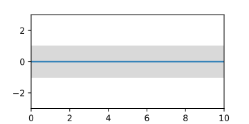 Prior Gaussian process, represented by the mean function and the area of the confidence interval.
 -
 posterior Gaussian process when three support points are known, represented by random curves.
 -
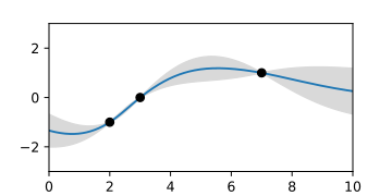 posterior Gaussian process, represented by the mean function and the area of the confidence interval.
 -
 posterior Gaussian process assuming measurement noise. The interpolations no longer pass through the points exactly.
 -
 posterior Gaussian process assuming measurement noise. The mean function becomes smoother and the confidence interval remains greater than zero.
 -
 posterior Gaussian process of the interpolation of a gap, represented by the mean function and the area of the confidence interval.
 -
 posterior Gaussian process of the interpolation of a gap, represented by animated random fluctuations according to the distribution.


The Python code for the examples can be found on the respective image description page.
Special cases
[edit | edit source]Underdetermined measurments
[edit | edit source]In some cases of conditional Gaussian processes, groups of linearly related measured values are completely indeterminate. E.g., this is the case for indirect measurements following from underdetermined equations, such as with a noninvertible positive semidefinite matrix of the form . The grid points then cannot be easily partitioned into known and unknown values, and the associated covariance matrix would be singular due to infinite uncertainties. This would correspond to a normal distribution that is infinitely stretched in certain spatial directions transverse to the coordinate axes. To account for the relationships between the undetermined variables, in such a case, the inverse matrix , called the precision matrix, must be used. This can describe completely undetermined measurements, which is expressed by zeros in the diagonal. For such a singular distribution with partially unknown measurements and singular measurement uncertainties , the wanted posterior distribution is obtained by the overlap to the prior Gaussian process model calculated by multiplying the probability densities. The union of the two normal distributions


is obtained by the Fusion operation after appropriate transformation, so that the singular of the two matrices remains inverse. The result is always a finite distribution, since the finite matrix dominates. If both are finite, the equation can be put into the form of the posterior Gaussian process as in the section on the conditional distribution.
Linear combination to a Gaussian process
[edit | edit source]From given basis functions a linear combination is to be formed, which has maximum overlap with the distribution of an associated Gaussian process . Or measured values are to be approximated, while the interfering signal , contained within, is ignored as far as possible. In both cases, the wanted coefficients can be calculated using generalized least squares estimation


The matrix contains the function values of the basis functions at the interpolation points . The resulting coefficients c with the associated covariance matrix describe the linear combination with the largest possible probability density in the distribution . The linear combination thereby approximates the mean function or the measured values in such a way that the residuals are best described by the covariance matrix . The method is used, for example, in the program library Scikit-learn to empirically estimate a polynomial mean function of a Gaussian process.


Approximation of an empirical Gaussian process
[edit | edit source]An empirically determined Gaussian process

![{\displaystyle k(t,t')={\frac {1}{N-1}}\sum _{p=1}^{N}\left[f_{p}(t)-m(t)\right]\cdot \left[f_{p}(t')-m(t')\right]}](https://wikimedia.org/api/rest_v1/media/math/render/svg/7f23777e5161267eaf143c21be846f58c2e93399)
from example functions with few distinct degrees of freedom can be approximated and simplified by means of the eigenvalue decomposition or singular value decomposition


of the covariance matrix . This is done by choosing the largest eigenvalues or singular values from the diagonal matrix . The corresponding columns of are the principal components of the Gaussian process (see Principal Component Analysis). If the columns are represented as functions , then the original Gaussian process is represented by the mean function and the covariance function


This Gaussian process describes exclusively functions of the linear combination
- ,

where each coefficient is scattered around zero mean as an independent random variable of variance .


Such a simplification is positively semidefinite and it usually lacks the properties to describe small-scale variations. These properties can be added to the covariance function in the form of a stationary covariance function fitted to the residuals:

Application examples
[edit | edit source]Example: Trend prediction
[edit | edit source]In a hypothetical application example from market research, the future demand for the topic "snowboard" is to be predicted. For this purpose, an extrapolation of the number of Google searches[15] on this term is to be calculated.
In the past data, one can see a periodic, but non-sinusoidal seasonal dependence, which can be explained by the winter in the northern hemisphere. Moreover, the trend decreased continuously over the last decade. In addition, one recognizes a recurring increase in search queries during the Olympic Games every four years. The covariance function was therefore modeled with a slow trend and a one- and four-year period:

The trend also appears to have a significant asymmetry. This can be the case if the underlying random effects do not add up but reinforce each other, resulting in a Log-Normal Distribution. However, the logarithm of such values describes a normal distribution, to which Gaussian process regression can be applied.

The figure shows an extrapolation of the curve (to the right of the dashed line). Since the results here were transformed back from the logarithmic plot using an exponential function, the predicted confidence intervals are correspondingly asymmetrical (gray area). The extrapolation plausibly shows the seasonal patterns and also the increase in searches for the Olympic Games every four years. The example with mixed properties demonstrates very well the versatile modeling possibilities of the Gaussian process regression, which are unified in a single interpolation method.
Python source code of the example calculation
Example: Sensor calibration
[edit | edit source]In an application example from industry, sensors are to be calibrated using Gaussian processes. Due to tolerances during manufacturing, the characteristic curves of the sensors show large individual differences. This causes high costs in calibration, since a complete characteristic curve would have to be measured for each sensor. However, the effort can be minimized by learning the exact behavior of the scattering by a Gaussian process. For this purpose, the complete characteristic curves of randomly selected representative sensors are measured and thus the Gaussian process of the scattering is calculated by


![{\displaystyle k(x,x')={\frac {1}{N-1}}\sum _{i=1}^{N}\left[f_{i}(x)-m(x)\right]\cdot \left[f_{i}(x')-m(x')\right]}](https://wikimedia.org/api/rest_v1/media/math/render/svg/113d714d79833fc992f5e4342a985b43f7c40a4e)
In the example shown, 15 representative characteristic curves are given. The resulting Gaussian process is represented by the mean function and the confidence interval .


With the conditional Gaussian process with


the complete characteristic map can now be reconstructed for each new sensor with a few individual measured values at the coordinates . The number of measured values must correspond at least to the number of degrees of freedom of the tolerances, which have an independent linear influence on the shape of the characteristic curve.

In the example shown, a single measured value is not yet sufficient to determine the characteristic curve unambiguously and precisely. The confidence interval shows the region of the curve which is not yet sufficiently accurate. With another measured value in this range, the remaining uncertainty can finally be completely eliminated. The exemplary fluctuations of the very differently acting sensors in this example thus seem to be caused by the tolerances of only two relevant inner degrees of freedom.


Python source code of the example calculation
Example: Signal decomposition
[edit | edit source]In a signal processing application example, a temporal signal is to be decomposed into its components. Let it be known about the system that the signal consists of three components following the three covariance functions


The sum signal then follows the addition rule of the covariance function
- .

The following two figures show three random signals which were generated and added for demonstration with these covariance functions. In the sum of the signals one can hardly recognize the periodic signal hidden in it with the naked eye, since its spectral range overlaps with that of the two other components.
-
 Single signals: Three randomly generated signals following certain Gaussian processes.
 -
 Sum: The sum of the three signals.


With the help of the operation decomposition the sum can be decomposed again into the three components


where . The estimate of the most likely decomposition shows how well the separation is possible in this case and how close the signals are to the original signals. The estimated uncertainties taking into account the cross-correlations are shown in the animation by random fluctuations.

-
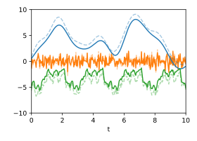 Decomposition: Most likely decomposition when the respective covariance functions are known. The original signals are shown dashed.
 -
 Uncertainty: Estimated uncertainties represented by animated random fluctuations corresponding to the (cross) covariance matrices.


The example shows how this method can be used to separate very different signals in one step. In contrast, other filtering methods such as moving averaging, Fourier filtering, polynomial regression, or spline approximation are optimized for specific signal characteristics and provide neither accurate error estimates nor cross-correlations.
If the Gaussian processes of the individual components for a given signal are not precisely known, then in some cases hypothesis testing can be performed using the log-marginal likelihood function, provided sufficient data are available to well-condition the function. Via its maximization, the parameters of the conjectured covariance functions can be fitted to the measured data.
Python source code of the example calculation
Literature
[edit | edit source]- C. E. Rasmussen. "Gaussian Processes in Machine Learning". doi:10.1007/978-3-540-28650-9_4.
{{cite journal}}: Cite journal requires|journal=(help) In: Olivier Bousquet (publisher): Advanced Lectures on Machine Learning. ML 2003. (= Lecture Notes in Computer Science. vol. 3176). Springer, Berlin/Heidelberg 2004.([1], pdf) - C. E. Rasmussen, C. K. I. Williams: Gaussian Processes for Machine Learning. MIT Press, 2006, ISBN 0-262-18253-X. (gaussianprocess.org, pdf)
- R. M. Dudley: Real Analysis and Probability. Wadsworth and Brooks/Cole, 1989.
- B. Simon: Functional Integration and Quantum Physics. Academic Press, 1979.
- M. L. Stein: Interpolation of Spatial Data: Some Theory for Kriging. Springer, 1999.
Weblinks
[edit | edit source]Educational material
[edit | edit source]- Gaussian Processes Web Site (Textbook, tutorials, code, etc.)
- Interactive demo on Gaussian process regression
- The Kernel Cookbook (Guide to the construction of covariance functions)
Software
[edit | edit source]- GPy – A Gaussian Process-Framework in Python
- Scikit Learn Gaussian Process – Gaussian process module of the machine learning library Scikit-learn for Python
- Gaussian process library written in C++11
References
[edit | edit source]- ↑ Kanagawa, M., Hennig, P., Sejdinovic, D., Sriperumbudur, B. K. (2018), Gaussian Processes and Kernel Methods: A Review on Connections and Equivalences, arXiv
{{citation}}: CS1 maint: uses authors parameter (link) - ↑ C. E. Rasmussen, C. K. I. Williams: Gaussian Processes for Machine Learning, Chapter 4.1 Preliminaries
- ↑ Topics in Probability: Gaussian Analysis, Math 7880-1, Spring 2015, University of Utah, Chapter 6 "Gaussian Processes", see Definition 1.7 for stationarity and Lemma 1.8 for translation invariance.
- ↑ C. E. Rasmussen, C. K. I. Williams: Gaussian Processes for Machine Learning. MIT Press, 2006, ISBN 0-262-18253-X, chapter 4.2 Examples of Covariance Functions, page 85
- ↑ C. E. Rasmussen, C. K. I. Williams: Gaussian Processes for Machine Learning. MIT Press, 2006, ISBN 0-262-18253-X, chapter 4.2 Examples of Covariance Functions, page 84
- ↑ C. E. Rasmussen, C. K. I. Williams: Gaussian Processes for Machine Learning MIT Press, 2006, ISBN 0-262-18253-X, Chapter 4.2.2 Dot Product Covariance Functions. p. 89 and Table 4.1, p. 94.
- ↑ C. E. Rasmussen, C. K. I. Williams: Gaussian Processes for Machine Learning. MIT Press, 2006, ISBN 0-262-18253-X, Chapter 4 "Covariance Functions", valid covariance functions are listed as "ND" in Table 4.1 on page 94.
- ↑ The derivation of the general linear transformation is based on the equation , by choosing the matrix F as [A B], as a vector ( ) and from corresponding four blocks.
- ↑ The derivation is based on the covariance rule for multiplication and associativity .
- ↑ The transformation involves, for example, multiplying by 1 = Σ1/Σ1 or adding 0 = Σ1-Σ1 and truncating the inverse matrices accordingly.
- ↑ Bar-Shalom, Yaakov; Campo, Leon (November 1986). "The Effect of the Common Process Noise on the Two-Sensor Fused-Track Covariance". IEEE Transactions on Aerospace and Electronic Systems. AES-22 (6): 803–805. doi:10.1109/TAES.1986.310815.
- ↑ The strategy corresponds to the a posteriori Gaussian process with measurement uncertainties, see the chapter on Gaussian process regression in the textbook C. E. Rasmussen, C. K. I. Williams: Processes for Machine Learning, Chapter 2 Regression. The Kalman filter also uses data fusion to separate signals and measurement uncertainties.
- ↑ C. E. Rasmussen, C. K. I. Williams: Gaussian Processes for Machine Learning, Chapter 4.2.4 Making New Kernels from Old. page 94.
- ↑ C. E. Rasmussen, C. K. I. Williams: Gaussian Processes for Machine Learning, Chapter 5.2 Bayesian Model Selection. page 108.
- ↑ The data is available at Google trends for the search term "snowboard".


