Fluid Mechanics Applications/A50:Optimisation of Intake Manifold of a Car
This project involves the optimisation of the intake manifold of a car where a special case of a Formula Society of Automotive Engineers vehicle has been considered. The car is a wheeled race vehicle designed to go from 0-100 kmph in under four seconds and have a top speed of about 140 kmph. The FSAE technical committee has an imposed a rule that the air flowing into the engine should pass through the 20mm diameter restriction. This is done to limit the power capability of the engine and induce uniformity in the engine performance of the various teams with different engine capacities. his involves the usage of a restrictor. The basic function of an air intake system is to provide the throttle bodies with air where it is then mixed with the fuel and sent to the combustion chamber. The construction of the intake system has a major influence on how the engine performs at various RPM’s.

Parts of the Intake Manifold[edit | edit source]
- Air Filter:In the Formula SAE car, it is the first and foremost component which is in contact with the atmosphere. Air enters the intake manifold through it and is carried through to the inlet of the engine. It filters the air so that minimum air impurities i.e. dust enter the intake system which may hamper engine performance.
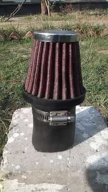
Air Filter of Intake Manifold - Throttle Body: The throttle valve is placed at the entrance of the air intake system, and it controls he behaviour of the engine and its power and performance. In compliance with the competition rules the throttle pedal is placed ahead of the air restrictor.

Throttle Body showing the Butterfly Valve 
Throttle body - Venturi: This the restrictor which is used. Of other restrictor options like: Orifice, Nozzle, venturi is the most suitable choice as it has the lowest

Vertical View of Venturi 
Horizontal view of Venturi - Plenum To prevent creation of vacuum in the engine since a restrictor is being used, hence a Plenum is used. The Plenum is the chamber or reservoir of air that supplies the engine.

Plenum showing venturi runner 
Plenum from another angle - Runner: The runners which are the tubes that feed the air from the plenum to the throttle bodies. Short runners give good top end speed whereas longer runners give good low end torque.
- Engine: The engine's cylinder can be regarded as the final destination of the air intake. Having passed through the entire intake system, the mixture of air and fuel mixture shall be inducted into the cylinder through the inlet valve.

Engine with the fuel injector and the sensors 
Engine and Throttle Body attached


.jpg)


Proposed Model[edit | edit source]
- Plenum: Cylindrical plenum is used due to manufacturing problems. Material used is brass and the plenum is made by brazing it. The dimensions of which are length 15.6 cm , diameter 10.4 cm
- Runner: It is a part of the plenum and has the same material. It is a uniform area pipe. It is a 10 cm long runner in which the fuel injector is infused as well to prevent any changes in the engine or any further tuning.
- Venturi: It is a convergent divergent nozzle with inner diameter 38 mm and outer diameter 44 mm and length 24 cm the CD angle is 156 deg. The material is aluminium for this due to us light weight and low friction factor.
Concepts Used[edit | edit source]
Bernoullis's Principle[edit | edit source]
In fluid dynamics, Bernoulli's principle states that for an inviscid flow of a nonconducting fluid, an increase in the speed of the fluid occurs simultaneously with a decrease in pressure or a decrease in the fluid's potential energy. The simple form of Bernoulli's principle is valid for incompressible flows (e.g. most liquid flows) and also for compressible flows (e.g. gases) moving at low Mach numbers (usually less than 0.3). In most flows of liquids, and of gases at low Mach number, the density of a fluid parcel can be considered to be constant, regardless of pressure variations in the flow. Therefore, the fluid can be considered to be incompressible and these flows are called incompressible flow. Bernoulli performed his experiments on liquids, so his equation in its original form is valid only for incompressible flow. A common form of Bernoulli's equation, valid at any arbitrary point along a streamline, is:
-
()

where:
- is the fluid flow speed at a point on a streamline,
- is the acceleration due to gravity,
- is the elevation of the point above a reference plane, with the positive z-direction pointing upward – so in the direction opposite to the gravitational acceleration,
- is the pressure at the chosen point, and
- is the density of the fluid at all points in the fluid.


For conservative force fields, Bernoulli's equation can be generalized as:[1]

where Ψ is the force potential at the point considered on the streamline. E.g. for the Earth's gravity Ψ = gz.
The following two assumptions must be met for this Bernoulli equation to apply:[1]
- the flow must be incompressible – even though pressure varies, the density must remain constant along a streamline;
- friction by viscous forces has to be negligible. In long lines mechanical energy dissipation as heat will occur. This loss can be estimated e.g. using Darcy–Weisbach equation.
By multiplying with the fluid density , equation (A) can be rewritten as:


or:

where:
- is dynamic pressure,

- is the piezometric head or hydraulic head (the sum of the elevation z and the pressure head)[2][3] and

- is the total pressure (the sum of the static pressure p and dynamic pressure q).[4]

The constant in the Bernoulli equation can be normalised. A common approach is in terms of total head or energy head H:

The above equations suggest there is a flow speed at which pressure is zero, and at even higher speeds the pressure is negative. Most often, gases and liquids are not capable of negative absolute pressure, or even zero pressure, so clearly Bernoulli's equation ceases to be valid before zero pressure is reached. In liquids – when the pressure becomes too low – cavitation occurs. The above equations use a linear relationship between flow speed squared and pressure. At higher flow speeds in gases, or for sound waves in liquid, the changes in mass density become significant so that the assumption of constant density is invalid.
However, it is important to remember that Bernoulli's principle does not apply in the boundary layer or in fluid flow through long pipes.
Applicability of incompressible flow equation to flow of gases[edit | edit source]
Bernoulli's equation is sometimes valid for the flow of gases: provided that there is no transfer of kinetic or potential energy from the gas flow to the compression or expansion of the gas. If both the gas pressure and volume change simultaneously, then work will be done on or by the gas. In this case, Bernoulli's equation – in its incompressible flow form – cannot be assumed to be valid. However if the gas process is entirely isobaric, or isochoric, then no work is done on or by the gas, (so the simple energy balance is not upset). According to the gas law, an isobaric or isochoric process is ordinarily the only way to ensure constant density in a gas. Also the gas density will be proportional to the ratio of pressure and absolute temperature, however this ratio will vary upon compression or expansion, no matter what non-zero quantity of heat is added or removed. The only exception is if the net heat transfer is zero, as in a complete thermodynamic cycle, or in an individual isentropic (frictionless adiabatic) process, and even then this reversible process must be reversed, to restore the gas to the original pressure and specific volume, and thus density. Only then is the original, unmodified Bernoulli equation applicable. In this case the equation can be used if the flow speed of the gas is sufficiently below the speed of sound, such that the variation in density of the gas (due to this effect) along each streamline can be ignored. Adiabatic flow at less than Mach 0.3 is generally considered to be slow enough.
In our case the flow is presumed to be steady and incompressible.
Pipe Flows[edit | edit source]
Calculate losses across the runners used in various spaces. There are two runners used one is of the same length as the throttle body. Thus one cones after the plenum, but is a part of it and attached to the engine cylinder head. The other comes after the venturi and it's attached to the plenum, it is used to allow easy fixing of the venturi on the plenum. Based on deducing the type of pipe (material, dimensions, and shape) we find out the pipe's Reynolds's number.If 0<Re<1000: laminar flow 1000<Re<infinity: turbulent flow
- ||

This is the formula applied to constant area pipes. Here hf is the frictional head loss in the pipe.
Minor Losses[edit | edit source]
Due to sudden expansion and contraction in the plenum there are losses which are minor losses and these can be calculated by taking the ratio of the head loss (hm = p/(rho g) ) through the devicwe to the velocity head (V2/(2g)) of the associated piping system: Loss Coefficient K = hm/ v2/(2g) = P/(1/2)rho V2 Although K is dimensionless, it is often not related to Reynold's number and roughness ratio but rather simply with raw size of the pipe. A single pipe may have several minor losses. Since all are correlated with V2/(2g) they can be summed into a single total system loss if the pipe is taken to have constant diameter: htot= hf +:m = {v^2/2g} (fl/d + )}}


Analysis[edit | edit source]
For the purpose of analysis of the flow ANSYS FLUENT is used. The flow simulation is done to understand the optimum convergent-divergent angle for the CD nozzle of the venturi. his angle influences the formation of Eddy and flow separation also the nature of flow whether is it laminar, chaotic laminar or turbulent. It helps us analyse the flow and thus make modulations in our design further. Flow simulation is done on ANSYS FLUENT by specifying a set of boundary conditions which influence the flow, and help deduce the flow form. Wide range of boundary conditions permit flow to enter and exit the solution domain.Defining boundary conditions involves:
- Identifying the location of the boundaries (e.g., inlets, walls, symmetry
- Supplying information at the boundaries
The data required at a boundary depends upon the boundary condition, type and the physical models employed. These conditions must be well known or reasonably approximated. Available Boundary Condition Types
External faces
- General – pressure inlet, pressure outlet
- Incompressible – velocity inlet, outflow
- Compressible – mass flow inlet, pressure farfield, mass flow outlet
- Other – wall, symmetry, axis, periodic
- Special – inlet vent, outlet vent, intake fan, exhaust fan
Cell zones
- Fluid
- Solid
- Porous media
- Heat exchanger
Internal faces
- Fan, interior, porous jump, radiator, wall
Also an important aspect is taking Axis Symmetric to reduce computational effort and also to reduce inputs and simplify flow field and geometry .
Proposed Experimental Analysis[edit | edit source]
To reach a valid conclusion and be case specific we can conduct a series of experiments which can aid us in deducing our
- Suction Pressure of the CBR 250 Engine used: Using a manometer which is open to air on one end and connected to the engine intake head with the help of rubber pipesso we get a differential pressure between the atmosphere and the suction pressure, we get the gauge pressure value.
- Pressure difference across the plenum: Using a manometer setup like used to calculate engine's suction pressure, to calculate the difference in pressure across the plenum, this would help in calculating the minor losses across the plenum.
- Pressure difference across the venturi: Using the same manometer used earlier the pressure difference can be again calculated, this will help to optimise the venturi design and calculate the converging-diverging angles through flow simulation on ANSYS Fluent. Via this, first the boundary pressure conditions across the venturi can be deduced, next, the flow model and pressure outlet conditions can be determined.
- Pressure difference across the throttle body: Using the same manometer and set up as above, this pressure difference will allow us to simulate the flow in the throttle body and give us suitable data to tune the engine as per our requirements.
- Flowrate across the venturi: Using an air box, with a flow meter (orifice) fitted inside, and using an inclined manometer, whose one side is connected to the inlet of the air box, and the other end at the outlet of the venturi, which is attached to the engine. With this we can measure the flow rate and the volumetric efficiency.
Doing so would aid us in deducing the pressure losses thus the losses across each element of the intake manifold. And would aid us in specifying the exact and not assumed values in the boundary conditions of flow simulation and thereby help us propose the most ideal design and shape of the Venturi, Plenum and Runner.
References[edit | edit source]
- ↑ a b Batchelor, G.K. (1967), §5.1, p. 265.
- ↑ Mulley, Raymond (2004). Flow of Industrial Fluids: Theory and Equations. CRC Press. ISBN 0-8493-2767-9.
{{cite book}}: CS1 maint: postscript (link), 410 pages. See pp. 43–44. - ↑ Chanson, Hubert (2004). Hydraulics of Open Channel Flow: An Introduction. Butterworth-Heinemann. ISBN 0-7506-5978-5.
{{cite book}}: CS1 maint: postscript (link), 650 pages. See p. 22. - ↑ Oertel, Herbert; Prandtl, Ludwig; Böhle, M.; Mayes, Katherine (2004). Prandtl's Essentials of Fluid Mechanics. Springer. pp. 70–71. ISBN 0-387-40437-6.
{{cite book}}: CS1 maint: postscript (link)