General Engineering Introduction/Error Analysis/Statistics Analysis
There are two ways to measure something:
- measure once the value, max and min (see measurement error)
- measure many times the value and compute using statistics the max and min
Random Error Assumption[edit | edit source]
There are two situations where measuring something many times to reduce random error is appropriate:
- at the beginning of the project where results are so chaotic, can not tell if improving, staying the same or growing worse.
- at the end of a project where trying to improve accuracy and can see clearly the affects of uncertainty.
Upper division and graduate level classes focus on how to use statistics at the end of a project. The goal here is to introduce statistics for use at the beginning of a project.
Average Concepts[edit | edit source]
- Mode -- the mode of the sequence 1,1,2,4,7 is 1. It occurs most frequently ... is not affected by extremes
- Median -- list all data, middle number is median is not affected extremes
- Mean -- the mean of the sequence, average 1,1,2,4,7 is 3. ... is affected by extremes
Outlier[edit | edit source]
Outliers are extremes. They can distort the mean computation. There is no rigid mathematical definition of what constitutes an outlier. Determining whether or not an observation is an outlier is ultimately a subjective exercise. Outliers more than three standard deviations need to be rationalized. The rationalization can result in those measurements being discarded.
Mean Calculation[edit | edit source]
The arithmetic mean is the "standard" average, often simply called the "mean".
For example, the arithmetic mean of five values: 4, 36, 45, 50, 75 is
Normal Distribution[edit | edit source]

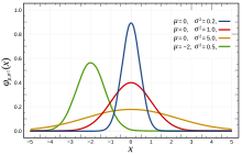
The observational error in an experiment is usually assumed to follow a normal distribution, and the propagation of uncertainty is computed using this assumption.
If the data is truly random, then when the value of X is 0 or μ = 0 and the standard deviation or σ 2 = 1 which is the red line in the graphic to the right.
Observational error could be due to a human error mixing chemicals in slightly different amounts; or using a physical device like a ruler that is going to give different values depending upon random positions of the head; or recording the same number off a digital thermometer at different times and wind conditions.
Obviously most things are not random, but they are random enough that this is a good, first level approximation of the error. It is a good starting point for understanding error and uncertainty computation.
Standard Deviation[edit | edit source]

Look at the results of two dart games. They both have the same average (the center of the board). Yet one dart game is obviously closer to the center than the other. How do we quantify this? A standard deviation (σ) quantifies this.
The goal here is to present an intuitive definition of standard deviation. So lets start off looking at two sequences of numbers:
- 1,1,2,4,7
- 2,2,3,3,5
Both have an average of . Obviously, the second sequence is closer to the average. The deviation of the first must be larger than deviation of the second. But adding up the deviation from the median and finding that average doesn't work:
Both deviations from the mean are 0. This isn't working because the negative is canceling out the positive. So how can we turn a negative number into a positive number? Square it and then take the square root. Or take absolute value:
Now we can see success. The first sequence 1,1,2,4,7 has a larger mean deviation than the second sequence 2,2,3,3,5. In general the mean deviation can be written:
The term "standard deviation" should read "root mean square deviation." It replaces the absolute signs with squares and then takes the square root of both the squared value and the number of samples. This makes the "standard deviation" larger (2 goes to 2.1, 0.8 goes to 1.2). This has a tendency to emphasize small differences and is preferred over the "mean deviation".
The problem with this technique (emphasizing small differences) is that it works only when the everything on the planet is sampled .. or the experiment is done infinitely number of times. The problems with it that lead to Bessel's correction:
The above formula is what is generally used inside of spreadsheet and computer algebra software because most of the time engineers and scientists are doing statistics on a sample of the possibilities, not all possibilities.
Interpreting the Standard Deviation[edit | edit source]
In most cases a small standard deviation or error is good. Here are some cases where the goal is to make the deviation big:
- Parables (everyone listens to the same thing, but interprets differently)
- Guitar Distortion
- Shifting a signal to a channel (distort like guitar, then filter off everything but a tiny sliver, then amplify into the channel)
- Rebalancing an Btree (spread data out so that new data can be added quickly)
- Many equilibrium points in a reaction, not one


