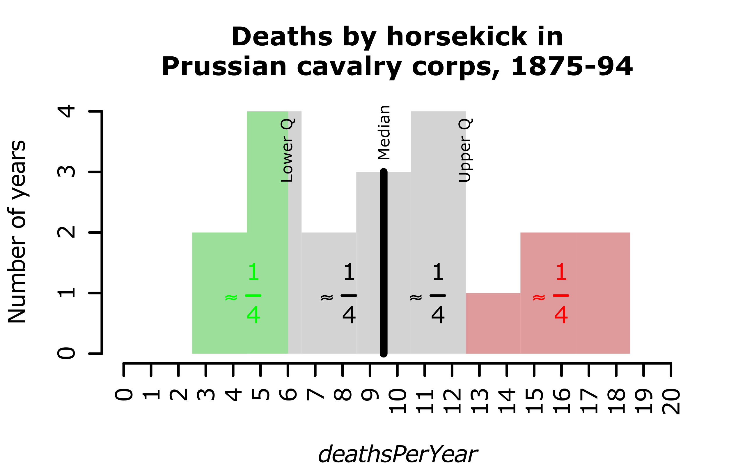
DescriptionR-horsekick totals-histogram+quartiles.svg	English: Histogram example with discrete data, with median line and quartiles marked by colour. Data = von Bortkiewicz's famous dataset of deaths by horse kick in Prussian cavalry corps
Date	6 March 2009
Source	Own work
Author	HYanWong
Permission (Reusing this file)	Public domainPublic domainfalsefalse I, the copyright holder of this work, release this work into the public domain. This applies worldwide. In some countries this may not be legally possible; if so: I grant anyone the right to use this work for any purpose, without any conditions, unless such conditions are required by law.

 

This W3C-unspecified chart was created with R.

using the following commands

svg(file = "R-horsekick_totals-histogram+quartiles.svg", width = 4, height = 2.5, pointsize = 8)
#Histogram example with discrete data, with median line and quartiles marked by colour. Data = von Bortkiewicz's famous dataset of deaths by horse kick in Prussian cavalry corps
library("pscl")
par(mar=c(4,4,4,2)+0.1)
X <- tapply(prussian$y, prussian$year, sum)
h <- hist(X, breaks=seq(2.5, 18.5, by=2), xlim=c(0,20), xlab=expression(italic("deathsPerYear")), xaxt="n", ylab="Number of years", main="Deaths by horsekick in\nPrussian cavalry corps, 1875-94", col="lightgrey", border=NA)
axis(1,0:20, las=2)

lowQ <- quantile(X, 0.25)
lowQ.x <- c(h$breaks[h$breaks < lowQ], lowQ)
lowQ.y <- h$counts[h$breaks <lowQ]
rect(lowQ.x[-length(lowQ.x)], 0, lowQ.x[-1], lowQ.y, col="#00FF0044", border=NA)
text(lowQ, max(h$counts), "Lower Q", srt=90, adj=1.1, cex=0.7)
text(mean(range(lowQ.x)), 1, expression(phantom(0) %~~% frac(1,4) * phantom(0)), col="green")

upQ <- quantile(X, 0.75)
upQ.x <- c(upQ, h$breaks[h$breaks > upQ]) 
upQ.y <- h$counts[(h$breaks > upQ)[-1]]
rect(upQ.x[-length(upQ.x)], 0, upQ.x[-1], upQ.y, col="#FF000044", border=NA)
text(upQ, max(h$counts), "Upper Q", srt=90, adj=1.1, cex=0.7)
text(mean(range(upQ.x)), 1, expression(phantom(0) %~~% frac(1,4) * phantom(0)), col="red")

med <- quantile(X, 0.5)
segments(med, 0, med, h$counts[findInterval(med,h$breaks)], lwd=3)
text(med, h$counts[findInterval(med,h$breaks)], "Median", srt=90, adj=-0.2, cex=0.7)
text(mean(c(max(lowQ.x), med)), 1, expression(phantom(0) %~~% frac(1,4) * phantom(0)))
text(mean(c(min(upQ.x), med)), 1, expression(phantom(0) %~~% frac(1,4) * phantom(0)))
dev.off()