Data Mining Algorithms In R/Clustering/Hierarchical Clustering

Introduction

A hierarchical clustering method consists of grouping data objects into a tree of clusters. There are two main types of techniques: a bottom-up and a top-down approach. The first one starts with small clusters composed by a single object and, at each step, merge the current clusters into greater ones, successively, until reach a cluster composed by all data objects. The second approach use the same logic, but to the opposite direction, starting with the greatest cluster, composed by all objects, and split it successively into smaller clusters until reach the singleton groups. Besides the strategies, other important issue is the metrics used to build (merge or split) clusters. Such metrics can be different distance measures, described next section.

Inter-cluster Metrics

Four widely used measures for distance between clusters are as follows. Where p and p' are two different data object points, m_i is the mean for cluster C_i, n_i is the number of objects in cluster C_i, and |p - p'| is the distance between p and p'.

Minimum distance: $d_{min}(C_{i},C_{j})=min_{p\in C_{i},p'\in C_{j}}\mid p-p'\mid$

Maximum distance: $d_{max}(C_{i},C_{j})=max_{p\in C_{i},p'\in C_{j}}\mid p-p'\mid$

Mean distance: $d_{mean}(C_{i},C_{j})=\mid m_{i}-m_{j}\mid$

Average distance: $d_{avg}(C_{i},C_{j})={\frac {1}{n_{i}n_{j}}}\sum _{p\in C_{i}}\sum _{p'\in C_{j}}\mid p-p'\mid$

Algorithms

One algorithm that implements the bottom-up approach is AGNES (AGglomerative NESting). The main idea of AGNES is, at its first step, create clusters composed by one single data object, and then, using a specified metric (such the ones mentioned previous section), merge such clusters into greater ones. The second step is repeated iteratively until only one cluster is obtained, composed by all data objects. Another example of algorithm implementing this approach is Cure, where instead dealing all the time with the whole set of entities, the clusters are shrank to its centers.

DIANA (DIvisive ANAlysis) is an example of an algorithm that implements top-down approach, starting with a single big cluster with all elements and iteratively spliting the current groups into smaller ones. As happens with AGNES and Cure, is necessary to define some metric to compute the distance inter-clusters, in order to decide how (where) they have to be splitted.

Implementation

In order to use Hierarchical Clustering algorithms in R, one must install cluster package. This package includes a function that performs the AGNES process and the DIANA process, according to different algorithms.

AGNES Function

The AGNES function provided by cluster package, might be used as follow:

agnes(x, diss = inherits(x, "dist"), metric = "euclidean", stand = FALSE, method = "average", par.method, keep.diss = n < 100, keep.data = !diss)

where the arguments are:

• x: data matrix or data frame (all variables must be numeric and missing values are allowed), or dissimilarity matrix (missing values aren't allowed), depending on the value of the diss argument.
• diss: logical flag. if TRUE (default for dist or dissimilarity objects), then x is assumed to be a dissimilarity matrix. If FALSE, then x is treated as a matrix of observations by variables.
• metric: character string specifying the metric to be used for calculating dissimilarities between observations. The currently available options are euclidean and manhattan. Euclidean distances are root sum-of-squares of differences, and manhattan distances are the sum of absolute differences. If x is already a dissimilarity matrix, then this argument will be ignored.
• stand: logical flag: if TRUE, then the measurements in x are standardized before calculating the dissimilarities. Measurements are standardized for each variable (column), by subtracting the variable’s mean value and dividing by the variable’s mean absolute deviation. If x is already a dissimilarity matrix, then this argument will be ignored.
• method: character string defining the clustering method. The six methods implemented are average ([unweighted pair-]group average method, UPGMA), single (single linkage), complete (complete linkage), ward (Ward’smethod), weighted (weighted average linkage) and its generalization flexible which uses (a constant version of) the Lance-Williams formula and the par.method argument. Default is average.
• par.method: if method = flexible, numeric vector of length 1, 3, or 4.
• keep.diss, keep.data: Logicals indicating if the dissimilarities and/or input data x should be kept in the result. Setting these to FALSE can give much smaller results and hence even save memory allocation time.

AGNES algorithm has the following features:

• yields the agglomerative coeficient which measures the amount of clustering structure found
• provides the hierarchical tree and the banner, a novel graphical display

The function AGNES returns a agnes object representing the clustering. This agnes object is a list with the components listed below:

• order: a vector giving a permutation of the original observations to allow for plotting
• order.lab: a vector similar to order, but containing observation labels instead of observation numbers. This component is only available if the original observations were labelled.
• height: a vector with the distances between merging clusters at the successive stages.
• ac: the agglomerative coefficient, measuring the clustering structure of the dataset.
• merge: an (n-1) by 2 matrix, where n is the number of observations.
• diss: an object of class dissimilarity, representing the total dissimilarity matrix of the dataset.
• data: a matrix containing the original or standardized measurements. This is available only if the input structure were different from a dissimilarity matrix.

Visualization

To visualize the AGNES function result might be used the functions: print and plot.

The first function simply print the components of object agnes and the second one plot the object, creating a chart that represents the data.

Here, it is an example of use function plot:

plot(x, ask = FALSE, which.plots = NULL, main = NULL,sub = paste("Agglomerative Coefficient = ",round(x$ac, digits = 2)),adj = 0, nmax.lab = 35, max.strlen = 5, xax.pretty = TRUE, ...)

The arguments used are:

• x: object agnes
• ask: If TRUE and which.plots = NULL, plot.agnes operates an interactive mode, via menu.
• which.plots: integer vector or NULL (default), the latter producing both plots
• main, sub: main and sub title for the plot, each with a convenient default.
• adj: For label adjustment in bannerplot
• nmax.lab: integer indicating the number of labels which is considered too large for singlename labelling the banner plot.
• max.strlen: positive integer giving the length to which strings are truncated in banner plot labeling.
• xax.prety: positive integer giving the length to which strings are truncated in banner plot labeling.
• ...: graphical parameters.

And here, it is the example of use function print:

print(x, ...)

The arguments are:

• x: object agnes
• ...: potential further arguments (require by generic function print)

DIANA Function

The DIANA function provided by cluster package, might be used as follow:

diana(x, diss = inherits(x, "dist"), metric = "euclidean", stand = FALSE, keep.diss = n < 100, keep.data = !diss)

where the arguments are:

• x: data matrix or data frame (all variables must be numeric and missing values are allowed), or dissimilarity matrix (missing values aren't allowed), depending on the value of the diss argument.
• diss: logical flag. if TRUE (default for dist or dissimilarity objects), then x is assumed to be a dissimilarity matrix. If FALSE, then x is treated as a matrix of observations by variables.
• metric: character string specifying the metric to be used for calculating dissimilarities between observations. The currently available options are euclidean and manhattan. Euclidean distances are root sum-of-squares of differences, and manhattan distances are the sum of absolute differences. If x is already a dissimilarity matrix, then this argument will be ignored.
• stand: logical; if true, the measurements in x are standardized before calculating the dissimilarities. Measurements are standardized for each variable (column), by subtracting the variable’s mean value and dividing by the variable’s mean absolute deviation. If x is already a dissimilarity matrix, then this argument will be ignored.
• keep.diss, keep.data: Logicals indicating if the dissimilarities and/or input data x should be kept in the

result. Setting these to FALSE can give much smaller results and hence even save memory allocation time.

DIANA algorithm is probably unique in computing a divisive hierarchy, whereas most other software for hierarchical clustering is ag glomerative. It has the same features as AGNES functions as follows:

• yields the agglomerative coeficient which measures the amount of clustering structure found
• provides the hierarchical tree and the banner, a novel graphical display

The function DIANA returns a diana object representing the clustering. This agnes object is a list with the components listed below:

• order: a vector giving a permutation of the original observations to allow for plotting
• order.lab: a vector similar to order, but containing observation labels instead of observation numbers. This component is only available if the original observations were labelled.
• heigh: a vector with the distances between merging clusters at the successive stages.
• dc: the divisive coefficient, measuring the clustering structure of the dataset.
• merge: an (n-1) by 2 matrix, where n is the number of observations.
• diss: an object of class dissimilarity, representing the total dissimilarity matrix of the dataset.
• data: a matrix containing the original or standardized measurements. This is available only if the input structure were different from a dissimilarity matrix.

Visualization

To visualize the DIANA function result might be used the functions: print and plot.

The first function simply print the components of object agnes and the second one plot the object, creating a chart that represents the data.

Here, it is an example of use function plot:

plot(x, ask = FALSE, which.plots = NULL, main = NULL, sub = paste("Divisive Coefficient = ", round(x$dc, digits = 2)), adj = 0, nmax.lab = 35, max.strlen = 5, xax.pretty = TRUE, ...)

The arguments used are:

• x: object diana
• ask: If TRUE and which.plots = NULL, plot.diana operates an interactive mode, via menu.
• which.plots: integer vector or NULL (default), the latter producing both plots
• main, sub: main and sub title for the plot, each with a convenient default.
• adj: For label adjustment in bannerplot
• nmax.lab: nteger indicating the number of labels which is considered too large for singlename labelling the banner plot.
• max.strlen: positive integer giving the length to which strings are truncated in banner plot labeling.
• xax.prety: positive integer giving the length to which strings are truncated in banner plot labeling.
• ...: graphical parameters.

And here, it is the example of use function print:

print(x, ...)

The arguments are:

• x: object diana
• ...: potential further arguments (require by generic function print)

Use Case

In this section it is illustrate an example of using hierarchical clustering in some Italian cities. In the example below, it is used mean distance, or single-linkage method.

Scenario

Given the distances in kilometers between Italian cities, the object is to group them into clusters in an agglomerative way. For examples in R is used the function agnes.

Input Data

The input data is a table containing the numeric values of distances between cities in Italy. The table consists of six columns (and rows), representing Italian cities. Each cell has a numeric value representing the distance in kilometers between them. The table can be loaded from a spreadsheet or from a text file.

Figure 1 illustres the cities used in this example.

• 
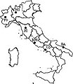  Figure 1

Input distance matrix

	BA	FI	MI	VO	RM	TO
BA	0	662	877	255	412	996
FI	662	0	295	468	268	400
MI	877	295	0	754	564	138
VO	255	468	754	0	219	869
RM	412	268	564	219	0	669
TO	996	400	138	869	669	0

Execution

The function agnes can be used to define the groups of countries as follow:

# import data
x <- read.table("data.txt")

# run AGNES
ag <- agnes (x, false, metric="euclidean", false, method ="single")
 
# print components of ag
print(ag)

# plot clusters
plot(ag, ask = FALSE, which.plots = NULL)

The value of the second parameter of agnes was FALSE, because x was treated as a matrix of observations by variables. The fourth parameter also is FALSE because isn't necessary standardizing each column.

Output

The result of printing the components of the class agnes returned by the function application is shown below:

Call:    agnes(x = x, diss = FALSE, metric = "euclidean", stand = FALSE,      method = "single") 
Agglomerative coefficient:  0.3370960 
Order of objects:
[1] BA VO RM FI MI TO
Height (summary):
   Min. 1st Qu.  Median    Mean 3rd Qu.    Max. 
  295.8   486.0   486.5   517.6   642.6   677.0 

Available components:
[1] "order"     "height"    "ac"        "merge"     "diss"      "call"     
[7] "method"    "order.lab" "data"

The result of plotting the class returned by the function application it is shown below:

• 
  Dendograma

Analysis

The algorithm always cluster the nearest pair of cities so, in this case, the " neighborhood " cities are clusterized first. In single link clustering the rule is that the distance from the compound object to another object is equal to the shortest distance from any member of the cluster to the outside object

However, there are a few weaknesses in agglomerative clustering methods:

• they do not scale well: time complexity of at least O($n^{2}$), where n is the number of total objects;
• they can never undo what was done previously.

References

J. Han and M. Kamber. Data Mining: Concepts and Techniuqes. Morgan Kaufmann Publishers, San Francisco, CA, 2006.

Maechler, M. Package 'cluster'. Disponível em <http://cran.r-project.org/web/packages/cluster/cluster.pdf> Acesso em 12 dez 2009.

Meira Jr., W.; Zaki, M. Fundamentals of Data Mining Algorithms. Disponível em <http://www.dcc.ufmg.br/miningalgorithms/DokuWiki/doku.php> Acesso em 12 dez 2009.

A Tutorial on Clustering Algorithms. Disponível em <http://home.dei.polimi.it/matteucc/Clustering/tutorial_html/hierarchical.html>. Acesso em 12 dez 2009.