Chemical Sciences: A Manual for CSIR-UGC National Eligibility Test for Lectureship and JRF/X-ray fluorescence

A Philips PW1606 X-ray fluorescence spectrometer with automated sample feed in a cement plant quality control laboratory

X-ray fluorescence (XRF) is the emission of characteristic "secondary" (or fluorescent) X-rays from a material that has been excited by bombarding with high-energy X-rays or gamma rays. The phenomenon is widely used for elemental analysis and chemical analysis, particularly in the investigation of metals, glass, ceramics and building materials, and for research in geochemistry, forensic science and archaeology.

The physics of XRF

Physics of X-ray fluorescence, in a schematic representation.

When materials are exposed to short-wavelength X-rays or to gamma rays, ionisation of their component atoms may take place. Ionisation consists of the ejection of one or more electrons from the atom, and may take place if the atom is exposed to radiation with an energy greater than its ionisation potential. X-rays and gamma rays can be energetic enough to expel tightly held electrons from the inner orbitals of the atom. The removal of an electron in this way renders the electronic structure of the atom unstable, and electrons in higher orbitals "fall" into the lower orbital to fill the hole left behind. In falling, energy is released in the form of a photon, the energy of which is equal to the energy difference of the two orbitals involved. Thus, the material emits radiation, which has energy characteristic of the atoms present. The term fluorescence is applied to phenomena in which the absorption of radiation of a specific energy results in the re-emission of radiation of a different energy (generally lower).

Figure 1: Electronic transitions in a calcium atom. Remember, when electrons are jumping down, one of the electrons in the lower orbital is missing.

Figure 2: Typical energy dispersive XRF spectrum

Figure 3: Spectrum of a rhodium target tube operated at 60 kV, showing continuous spectrum and K lines

Characteristic radiation

Each element has electronic orbitals of characteristic energy. Following removal of an inner electron by an energetic photon provided by a primary radiation source, an electron from an outer shell drops into its place. There are a limited number of ways in which this can happen, as shown in figure 1. The main transitions are given names: an L→K transition is traditionally called Kα, an M→K transition is called Kβ, an M→L transition is called Lα, and so on. Each of these transitions yields a fluorescent photon with a characteristic energy equal to the difference in energy of the initial and final orbital. The wavelength of this fluorescent radiation can be calculated from Planck's Law:

$\lambda =h\cdot c/E$

The fluorescent radiation can be analysed either by sorting the energies of the photons (energy-dispersive analysis) or by separating the wavelengths of the radiation (wavelength-dispersive analysis). Once sorted, the intensity of each characteristic radiation is directly related to the amount of each element in the material. This is the basis of a powerful technique in analytical chemistry. Figure 2 shows the typical form of the sharp fluorescent spectral lines obtained in the wavelength-dispersive method (see Moseley's law).

Primary radiation

In order to excite the atoms, a source of radiation is required, with sufficient energy to expel tightly held inner electrons. Conventional X-ray generators are most commonly used, because their output can readily be "tuned" for the application, and because higher power can be deployed relative to other techniques. However, gamma ray sources can be used without the need for an elaborate power supply, allowing an easier use in small portable instruments. When the energy source is a synchrotron or the X-ray are focussed by an optic like a polycapillary, the X-ray beam can be very small and very intense. As a result, atomic information on the sub-micrometer scale can be obtained. X-ray generators in the range 20–60 kV in order to the K line, which allows excitation of a broad range of atoms. The continuous spectrum consists of "bremsstrahlung" radiation: radiation produced when high energy electrons passing through the tube are progressively decelerated by the material of the tube anode (the "target"). A typical tube output spectrum is shown in figure 3.

Dispersion

In energy dispersive analysis, the fluorescent X-rays emitted by the material sample are directed into a solid-state detector which produces a "continuous" distribution of pulses, the voltages of which are proportional to the incoming photon energies. This signal is processed by a multichannel analyser (MCA) which produces an accumulating digital spectrum that can be processed to obtain analytical data. In wavelength dispersive analysis, the fluorescent X-rays emitted by the material sample are directed into a diffraction grating monochromator. The diffraction grating used is usually a single crystal. By varying the angle of incidence and take-off on the crystal, a single X-ray wavelength can be selected. The wavelength obtained is given by the Bragg Equation:

$n\cdot \lambda =2d\cdot \sin(\theta )$

where d is the spacing of atomic layers parallel to the crystal surface.

Detection

In energy dispersive analysis, dispersion and detection are a single operation, as already mentioned above. Proportional counters or various types of solid state detectors (PIN diode, Si(Li), Ge(Li), Silicon Drift Detector SDD) are used. They all share the same detection principle: An incoming X-ray photon ionises a large number of detector atoms with the amount of charge produced being proportional to the energy of the incoming photon. The charge is then collected and the process repeats itself for the next photon. Detector speed is obviously critical, as all charge carriers measured have to come from the same photon to measure the photon energy correctly (peak length discrimination is used to eliminate events that seem to have been produced by two X-ray photons arriving almost simultaneously). The spectrum is then built up by dividing the energy spectrum into discreet bins and counting the number of pulses registered within each energy bin. EDXRF detector types vary in resolution, speed and the means of cooling (a low number of free charge carriers is critical in the solid state detectors): proportional counters with resolutions of several hundred eV cover the low end of the performance spectrum, followed by PIN diode detectors, while the Si(Li), Ge(Li) and Silicon Drift Detectors (SDD) occupy the high end of the performance scale.

In wavelength dispersive analysis, the single-wavelength radiation produced by the monochromator is passed into a photomultiplier, a detector similar to a Geiger counter, which counts individual photons as they pass through. The counter is a chamber containing a gas that is ionised by X-ray photons. A central electrode is charged at (typically) +1700 V with respect to the conducting chamber walls, and each photon triggers a pulse-like cascade of current across this field. The signal is amplified and transformed into an accumulating digital count. These counts are then processed to obtain analytical data.

X-ray intensity

The fluorescence process is inefficient, and the secondary radiation is much weaker than the primary beam. Furthermore, the secondary radiation from lighter elements is of relatively low energy (long wavelength) and has low penetrating power, and is severely attenuated if the beam passes through air for any distance. Because of this, for high-performance analysis, the path from tube to sample to detector is maintained under high vacuum (around 10 Pa residual pressure). This means in practice that most of the working parts of the instrument have to be located in a large vacuum chamber. The problems of maintaining moving parts in vacuo, and of rapidly introducing and withdrawing the sample without losing vacuum, pose major challenges for the design of the instrument. For less demanding applications, or when the sample is damaged by a vacuum (e.g. a volatile sample), a helium-swept X-ray chamber can be substituted, with some loss of low-Z (Z = atomic number) intensities.

XRF in chemical analysis

The use of a primary X-ray beam to excite fluorescent radiation from the sample was first proposed by Glocker and Schreiber in 1928. Today, the method is used as a non-destructive analytical technique, and as a process control tool in many extractive and processing industries. In principle, the lightest element that can be analysed is beryllium (Z = 4), but due to instrumental limitations and low X-ray yields for the light elements, it is often difficult to quantify elements lighter than sodium (Z = 11), unless background corrections and very comprehensive interelement corrections are made.

Figure 4: Schematic arrangement of EDX spectrometer

Energy dispersive spectrometry

In energy dispersive spectrometers (EDX or EDS), the detector allows the determination of the energy of the photon when it is detected. Detectors historically have been based on silicon semiconductors, in the form of lithium-drifted silicon crystals, or high-purity silicon wafers.

Figure 5: Schematic form of a Si(Li) detector

Si(Li) detectors

These consist essentially of a 3–5 mm thick silicon junction type p-i-n diode (same as PIN diode) with a bias of -1000 V across it. The lithium-drifted centre part forms the non-conducting i-layer, where Li compensates the residual acceptors which would otherwise make the layer p-type. When an X-ray photon passes through, it causes a swarm of electron-hole pairs to form, and this causes a voltage pulse. To obtain sufficiently low conductivity, the detector must be maintained at low temperature, and liquid-nitrogen must be used for the best resolution. With some loss of resolution, the much more convenient Peltier cooling can be employed.

Wafer detectors

More recently, high-purity silicon wafers with low conductivity have become routinely available. Cooled by the Peltier effect, this provides a cheap and convenient detector, although the liquid nitrogen cooled Si(Li) detector still has the best resolution (i.e. ability to distinguish different photon energies).

Amplifiers

The pulses generated by the detector are processed by pulse-shaping amplifiers. It takes time for the amplifier to shape the pulse for optimum resolution, and there is therefore a trade-off between resolution and count-rate: long processing time for good resolution results in "pulse pile-up" in which the pulses from successive photons overlap. Multi-photon events are, however, typically more drawn out in time (photons did not arrive exactly at the same time) than single photon events and pulse-length discrimination can thus be used to filter most of these out. Even so, a small number of pile-up peaks will remain and pile-up correction should be built into the software in applications that require trace analysis. To make the most efficient use of the detector, the tube current should be reduced to keep multi-photon events (before discrimination) at a reasonable level, e.g. 5–20%.

Processing

Considerable computer power is dedicated to correcting for pulse-pile up and for extraction of data from poorly resolved spectra. These elaborate correction processes tend to be based on empirical relationships that may change with time, so that continuous vigilance is required in order to obtain chemical data of adequate precision.

Usage

EDX spectrometers are superior to WDX spectrometers in that they are smaller, simpler in design and have fewer engineered parts. They can also use miniature X-ray tubes or gamma sources. This makes them cheaper and allows miniaturization and portability. This type of instrument is commonly used for portable quality control screening applications, such as testing toys for Lead (Pb) content, sorting scrap metals, and measuring the lead content of residential paint. On the other hand, the low resolution and problems with low count rate and long dead-time makes them inferior for high-precision analysis. They are, however, very effective for high-speed, multi-elemental analysis. Field Portable XRF analysers currently on the market weigh less than 2 kg, and have limits of detection on the order of 2 parts per million of Lead (Pb) in pure sand.

Figure 6: Schematic arrangement of wavelength dispersive spectrometer

Chemist operates a goniometer used for X-ray fluorescence analysis of individual grains of mineral specimens, U.S. Geological Survey, 1958.

Wavelength dispersive spectrometry

In wavelength dispersive spectrometers (WDX or WDS), the photons are separated by diffraction on a single crystal before being detected. Although wavelength dispersive spectrometers are occasionally used to scan a wide range of wavelengths, producing a spectrum plot as in EDS, they are usually set up to make measurements only at the wavelength of the emission lines of the elements of interest. This is achieved in two different ways:

• "Simultaneous" spectrometers have a number of "channels" dedicated to analysis of a single element, each consisting of a fixed-geometry crystal monochromator, a detector, and processing electronics. This allows a number of elements to be measured simultaneously, and in the case of high-powered instruments, complete high-precision analyses can be obtained in under 30 s. Another advantage of this arrangement is that the fixed-geometry monochromators have no continuously moving parts, and so are very reliable. Reliability is important in production environments where instruments are expected to work without interruption for months at a time. Disadvantages of simultaneous spectrometers include relatively high cost for complex analyses, since each channel used is expensive. The number of elements that can be measured is limited to 15–20, because of space limitations on the number of monochromators that can be crowded around the fluorescing sample. The need to accommodate multiple monochromators means that a rather open arrangement around the sample is required, leading to relatively long tube-sample-crystal distances, which leads to lower detected intensities and more scattering. The instrument is inflexible, because if a new element is to be measured, a new measurement channel has to be bought and installed.

• "Sequential" spectrometers have a single variable-geometry monochromator (but usually with an arrangement for selecting from a choice of crystals), a single detector assembly (but usually with more than one detector arranged in tandem), and a single electronic pack. The instrument is programmed to move through a sequence of wavelengths, in each case selecting the appropriate X-ray tube power, the appropriate crystal, and the appropriate detector arrangement. The length of the measurement program is essentially unlimited, so this arrangement is very flexible. Because there is only one monochromator, the tube-sample-crystal distances can be kept very short, resulting in minimal loss of detected intensity. The obvious disadvantage is relatively long analysis time, particularly when many elements are being analysed, not only because the elements are measured in sequence, but also because a certain amount of time is taken in readjusting the monochromator geometry between measurements. Furthermore, the frenzied activity of the monochromator during an analysis program is a challenge for mechanical reliability. However, modern sequential instruments can achieve reliability almost as good as that of simultaneous instruments, even in continuous-usage applications.

Sample presentation

In order to keep the geometry of the tube-sample-detector assembly constant, the sample is normally prepared as a flat disc, typically of diameter 20–50 mm. This is located at a standardized, small distance from the tube window. Because the X-ray intensity follows an inverse-square law, the tolerances for this placement and for the flatness of the surface must be very tight in order to maintain a repeatable X-ray flux. Ways of obtaining sample discs vary: metals may be machined to shape, minerals may be finely ground and pressed into a tablet, and glasses may be cast to the required shape. A further reason for obtaining a flat and representative sample surface is that the secondary X-rays from lighter elements often only emit from the top few micrometers of the sample. In order to further reduce the effect of surface irregularities, the sample is usually spun at 5–20 rpm. It is necessary to ensure that the sample is sufficiently thick to absorb the entire primary beam. For higher-Z materials, a few millimetres thickness is adequate, but for a light-element matrix such as coal, a thickness of 30–40 mm is needed.

Figure 7: Bragg diffraction condition

Monochromators

The common feature of monochromators is the maintenance of a symmetrical geometry between the sample, the crystal and the detector. In this geometry the Bragg diffraction condition is obtained.

The X-ray emission lines are very narrow (see figure 2), so the angles must be defined with considerable precision. This is achieved in two ways:

• Flat crystal with Soller collimators

The Soller collimator is a stack of parallel metal plates, spaced a few tenths of a millimetre apart. To improve angle resolution, one must lengthen the collimator, and/or reduce the plate spacing. This arrangement has the advantage of simplicity and relatively low cost, but the collimators reduce intensity and increase scattering, and reduce the area of sample and crystal that can be "seen". The simplicity of the geometry is especially useful for variable-geometry monochromators.

• 
  Figure 8: Flat crystal with Soller collimators
• 
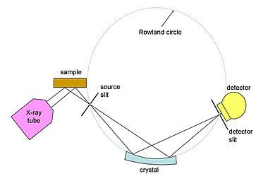  Figure 9: Curved crystal with slits

• Curved crystal with slits

The Rowland circle geometry ensures that the slits are both in focus, but in order for the Bragg condition to be met at all points, the crystal must first be bent to a radius of 2R (where R is the radius of the Rowland circle), then ground to a radius of R. This arrangement allows higher intensities (typically 8-fold) with higher resolution (typically 4-fold) and lower background. However, the mechanics of keeping Rowland circle geometry in a variable-angle monochromator is extremely difficult. In the case of fixed-angle monochromators (for use in simultaneous spectrometers), crystals bent to a logarithmic spiral shape give the best focusing performance. The manufacture of curved crystals to acceptable tolerances increases their price considerably.

Analysis Lines

The spectral lines used for chemical analysis are selected on the basis of intensity, accessibility by the instrument, and lack of line overlaps. Typical lines used, and their wavelengths, are as follows:

element	line	wavelength (nm)		element	line	wavelength (nm)		element	line	wavelength (nm)		element	line	wavelength (nm)
Li	Kα	22.8		Ni	Kα1	0.1658		I	Lα1	0.3149		Pt	Lα1	0.1313
Be	Kα	11.4		Cu	Kα1	0.1541		Xe	Lα1	0.3016		Au	Lα1	0.1276
B	Kα	6.76		Zn	Kα1	0.1435		Cs	Lα1	0.2892		Hg	Lα1	0.1241
C	Kα	4.47		Ga	Kα1	0.1340		Ba	Lα1	0.2776		Tl	Lα1	0.1207
N	Kα	3.16		Ge	Kα1	0.1254		La	Lα1	0.2666		Pb	Lα1	0.1175
O	Kα	2.362		As	Kα1	0.1176		Ce	Lα1	0.2562		Bi	Lα1	0.1144
F	Kα1,2	1.832		Se	Kα1	0.1105		Pr	Lα1	0.2463		Po	Lα1	0.1114
Ne	Kα1,2	1.461		Br	Kα1	0.1040		Nd	Lα1	0.2370		At	Lα1	0.1085
Na	Kα1,2	1.191		Kr	Kα1	0.09801		Pm	Lα1	0.2282		Rn	Lα1	0.1057
Mg	Kα1,2	0.989		Rb	Kα1	0.09256		Sm	Lα1	0.2200		Fr	Lα1	0.1031
Al	Kα1,2	0.834		Sr	Kα1	0.08753		Eu	Lα1	0.2121		Ra	Lα1	0.1005
Si	Kα1,2	0.7126		Y	Kα1	0.08288		Gd	Lα1	0.2047		Ac	Lα1	0.0980
P	Kα1,2	0.6158		Zr	Kα1	0.07859		Tb	Lα1	0.1977		Th	Lα1	0.0956
S	Kα1,2	0.5373		Nb	Kα1	0.07462		Dy	Lα1	0.1909		Pa	Lα1	0.0933
Cl	Kα1,2	0.4729		Mo	Kα1	0.07094		Ho	Lα1	0.1845		U	Lα1	0.0911
Ar	Kα1,2	0.4193		Tc	Kα1	0.06751		Er	Lα1	0.1784		Np	Lα1	0.0888
K	Kα1,2	0.3742		Ru	Kα1	0.06433		Tm	Lα1	0.1727		Pu	Lα1	0.0868
Ca	Kα1,2	0.3359		Rh	Kα1	0.06136		Yb	Lα1	0.1672		Am	Lα1	0.0847
Sc	Kα1,2	0.3032		Pd	Kα1	0.05859		Lu	Lα1	0.1620		Cm	Lα1	0.0828
Ti	Kα1,2	0.2749		Ag	Kα1	0.05599		Hf	Lα1	0.1570		Bk	Lα1	0.0809
V	Kα1	0.2504		Cd	Kα1	0.05357		Ta	Lα1	0.1522		Cf	Lα1	0.0791
Cr	Kα1	0.2290		In	Lα1	0.3772		W	Lα1	0.1476		Es	Lα1	0.0773
Mn	Kα1	0.2102		Sn	Lα1	0.3600		Re	Lα1	0.1433		Fm	Lα1	0.0756
Fe	Kα1	0.1936		Sb	Lα1	0.3439		Os	Lα1	0.1391		Md	Lα1	0.0740
Co	Kα1	0.1789		Te	Lα1	0.3289		Ir	Lα1	0.1351		No	Lα1	0.0724

Other lines are often used, depending on the type of sample and equipment available.

Crystals

The desirable characteristics of a diffraction crystal are:

• High diffraction intensity
• High dispersion
• Narrow diffracted peak width
• High peak-to-background
• Absence of interfering elements
• Low thermal coefficient of expansion
• Stability in air and on exposure to X-rays
• Ready availability
• Low cost

Crystals with simple structure tend to give the best diffraction performance. Crystals containing heavy atoms can diffract well, but also fluoresce themselves, causing interference. Crystals that are water-soluble, volatile or organic tend to give poor stability.

Commonly used crystal materials include LiF (lithium fluoride), ADP (ammonium dihydrogen phosphate), Ge (germanium), graphite, InSb (indium antimonide), PE (tetrakis-(hydroxymethyl)-methane: penta-erythritol), KAP (potassium hydrogen phthalate), RbAP (rubidium hydrogen phthalate) and TlAP (thallium(I) hydrogen phthalate). In addition, there is an increasing use of "layered synthetic microstructures", which are "sandwich" structured materials comprising successive thick layers of low atomic number matrix, and monoatomic layers of a heavy element. These can in principle be custom-manufactured to diffract any desired long wavelength, and are used extensively for elements in the range Li to Mg.

Properties of commonly used crystals

material	plane	d (nm)	min λ (nm)	max λ (nm)	intensity	thermal expansion	durability
LiF	200	0.2014	0.053	0.379	+++++	+++	+++
LiF	220	0.1424	0.037	0.268	+++	++	+++
LiF	420	0.0901	0.024	0.169	++	++	+++
ADP	101	0.5320	0.139	1.000	+	++	++
Ge	111	0.3266	0.085	0.614	+++	+	+++
graphite	001	0.3354	0.088	0.630	++++	+	+++
InSb	111	0.3740	0.098	0.703	++++	+	+++
PE	002	0.4371	0.114	0.821	+++	+++++	+
KAP	1010	1.325	0.346	2.490	++	++	++
RbAP	1010	1.305	0.341	2.453	++	++	++
Si	111	0.3135	0.082	0.589	++	+	+++
TlAP	1010	1.295	0.338	2.434	+++	++	++
6 nm LSM	-	6.00	1.566	11.276	+++	+	++

Detectors

Detectors used for wavelength dispersive spectrometry need to have high pulse processing speeds in order to cope with the very high photon count rates that can be obtained. In addition, they need sufficient energy resolution to allow filtering-out of background noise and spurious photons from the primary beam or from crystal fluorescence. There are four common types of detector:

• gas flow proportional counters
• sealed gas detectors
• scintillation counters
• semiconductor detectors

Figure 10: Arrangement of gas flow proportional counter

Gas flow proportional counters are used mainly for detection of longer wavelengths. Gas flows through it continuously. Where there are multiple detectors, the gas is passed through them in series, then led to waste. The gas is usually 90% argon, 10% methane ("P10"), although the argon may be replaced with neon or helium where very long wavelengths (over 5 nm) are to be detected. The argon is ionised by incoming X-ray photons, and the electric field multiplies this charge into a measurable pulse. The methane suppresses the formation of fluorescent photons caused by recombination of the argon ions with stray electrons. The anode wire is typically tungsten or nichrome of 20–60 μm diameter. Since the pulse strength obtained is essentially proportional to the ratio of the detector chamber diameter to the wire diameter, a fine wire is needed, but it must also be strong enough to be maintained under tension so that it remains precisely straight and concentric with the detector. The window needs to be conductive, thin enough to transmit the X-rays effectively, but thick and strong enough to minimize diffusion of the detector gas into the high vacuum of the monochromator chamber. Materials often used are beryllium metal, aluminised PET film and aluminised polypropylene. Ultra-thin windows (down to 1 μm) for use with low-penetration long wavelengths are very expensive. The pulses are sorted electronically by "pulse height selection" in order to isolate those pulses deriving from the secondary X-ray photons being counted.

Sealed gas detectors are similar to the gas flow proportional counter, except that the gas does not flow though it. The gas is usually krypton or xenon at a few atmospheres pressure. They are applied usually to wavelengths in the 0.15–0.6 nm range. They are applicable in principle to longer wavelengths, but are limited by the problem of manufacturing a thin window capable of withstanding the high pressure difference.

Scintillation counters consist of a scintillating crystal (typically of sodium iodide doped with thallium) attached to a photomultiplier. The crystal produces a group of scintillations for each photon absorbed, the number being proportional to the photon energy. This translates into a pulse from the photomultiplier of voltage proportional to the photon energy. The crystal must be protected with a relatively thick aluminium/beryllium foil window, which limits the use of the detector to wavelengths below 0.25 nm. Scintillation counters are often connected in series with a gas flow proportional counter: the latter is provided with an outlet window opposite the inlet, to which the scintillation counter is attached. This arrangement is particularly used in sequential spectrometers.

Semiconductor detectors can be used in theory, and their applications are increasing as their technology improves, but historically their use for WDX has been restricted by their slow response (see EDX).

A glass "bead" specimen for XRF analysis being cast at around 1100 °C in a Herzog automated fusion machine in a cement plant quality control laboratory. 1 (top): fusing, 2: preheating the mould, 3: pouring the melt, 4: cooling the "bead"

Extracting analytical results

At first sight, the translation of X-ray photon count-rates into elemental concentrations would appear to be straightforward: WDX separates the X-ray lines efficiently, and the rate of generation of secondary photons is proportional to the element concentration. However, the number of photons leaving the sample is also affected by the physical properties of the sample: so-called "matrix effects". These fall broadly into three categories:

• X-ray absorption
• X-ray enhancement
• sample macroscopic effects

All elements absorb X-rays to some extent. Each element has a characteristic absorption spectrum which consists of a "saw-tooth" succession of fringes, each step-change of which has wavelength close to an emission line of the element. Absorption attenuates the secondary X-rays leaving the sample. For example, the mass absorption coefficient of silicon at the wavelength of the aluminium Kα line is 50 m²/kg, whereas that of iron is 377 m²/kg. This means that a given concentration of aluminium in a matrix of iron gives only one seventh of the count rate compared with the same concentration of aluminium in a silicon matrix. Fortunately, mass absorption coefficients are well known and can be calculated. However, to calculate the absorption for a multi-element sample, the composition must be known. For analysis of an unknown sample, an iterative procedure is therefore used. It will be noted that, to derive the mass absorption accurately, data for the concentration of elements not measured by XRF may be needed, and various strategies are employed to estimate these. As an example, in cement analysis, the concentration of oxygen (which is not measured) is calculated by assuming that all other elements are present as standard oxides.

Enhancement occurs where the secondary X-rays emitted by a heavier element are sufficiently energetic to stimulate additional secondary emission from a lighter element. This phenomenon can also be modelled, and corrections can be made provided that the full matrix composition can be deduced.

Sample macroscopic effects consist of effects of inhomogeneities of the sample, and unrepresentative conditions at its surface. Samples are ideally homogeneous and isotropic, but they often deviate from this ideal. Mixtures of multiple crystalline components in mineral powders can result in absorption effects that deviate from those calculable from theory. When a powder is pressed into a tablet, the finer minerals concentrate at the surface. Spherical grains tend to migrate to the surface more than do angular grains. In machined metals, the softer components of an alloy tend to smear across the surface. Considerable care and ingenuity are required to minimize these effects. Because they are artefacts of the method of sample preparation, these effects can not be compensated by theoretical corrections, and must be "calibrated in". This means that the calibration materials and the unknowns must be compositionally and mechanically similar, and a given calibration is applicable only to a limited range of materials. Glasses most closely approach the ideal of homogeneity and isotropy, and for accurate work, minerals are usually prepared by dissolving them in a borate glass, and casting them into a flat disc or "bead". Prepared in this form, a virtually universal calibration is applicable.

Further corrections that are often employed include background correction and line overlap correction. The background signal in an XRF spectrum derives primarily from scattering of primary beam photons by the sample surface. Scattering varies with the sample mass absorption, being greatest when mean atomic number is low. When measuring trace amounts of an element, or when measuring on a variable light matrix, background correction becomes necessary. This is really only feasible on a sequential spectrometer. Line overlap is a common problem, bearing in mind that the spectrum of a complex mineral can contain several hundred measurable lines. Sometimes it can be overcome by measuring a less-intense, but overlap-free line, but in certain instances a correction is inevitable. For instance, the Kα is the only usable line for measuring sodium, and it overlaps the zinc Lβ (L₂-M₄) line. Thus zinc, if present, must be analysed in order to properly correct the sodium value.

Other spectroscopic methods using the same principle

It is also possible to create a characteristic secondary X-ray emission using other incident radiation to excite the sample:

• electron beam: electron microprobe (or Castaing microprobe);
• ion beam: particle induced X-ray emission (PIXE).

When radiated by an X-ray beam, the sample also emits other radiations that can be used for analysis:

• electrons ejected by the photoelectric effect: X-ray photoelectron spectroscopy (XPS), also called electron spectroscopy for chemical analysis (ESCA)

The de-excitation also ejects Auger electrons, but Auger electron spectroscopy (AES) normally uses an electron beam as the probe.

Confocal microscopy X-ray fluorescence imaging is a newer technique that allow control over depth, in addition to horizontal and vertical aiming, for example, when analyzing buried layers in a painting.

Instrument qualification

A 2001 review, addresses the application of portable instrumentation from QA/QC perspectives. It provides a guide to the development of a set of SOPs if regulatory compliance guidelines are not available.

Further information: Verification and Validation

See also

• Emission spectroscopy
• List of materials analysis methods
• Micro-X-ray fluorescence
• X-ray fluorescence holography

References

• Beckhoff, B., Kanngießer, B., Langhoff, N., Wedell, R., Wolff, H., Handbook of Practical X-Ray Fluorescence Analysis, Springer, 2006, ISBN 3-540-28603-9
• Bertin, E. P., Principles and Practice of X-ray Spectrometric Analysis, Kluwer Academic / Plenum Publishers, ISBN 0-3063-0809-6
• Buhrke, V. E., Jenkins, R., Smith, D. K., A Practical Guide for the Preparation of Specimens for XRF and XRD Analysis, Wiley, 1998, ISBN 0-471-19458-1
• Jenkins, R., X-ray Fluorescence Spectrometry, Wiley, ISBN 0-4712-9942-1
• Jenkins, R., De Vries, J. L., Practical X-ray Spectrometry, Springer-Verlag, 1973, ISBN 0387910298
• Jenkins, R., R.W. Gould, R. W., Gedcke, D., Quantitative X-ray Spectrometry, Marcel Dekker, ISBN 0-8247-9554-7
• Van Grieken, R. E., Markowicz, A. A., Handbook of X-Ray Spectrometry 2nd ed.; Marcel Dekker Inc: New York, 2002; Vol. 29; ISBN 0-8247-0600-5